Multi-model method for solving nonlinear transient inverse heat conduction problems

Abstract

The multi-model inverse method for nonlinear inverse problems is established based on the multi-model control theory. First the model switching variable is chosen and several typical operating balance points in the workspace of the balance variable are selected. Then for each operating balance point the linear local model is established, and the local controller is designed for each linear local model. Finally, according to the instantaneous matching degree between the actual model and the local models, the inversion results of each local controller are weighted and synthesized to obtain the final inversion result. Numerical tests are implemented to solve the one-dimensional nonlinear inverse heat conduction problem by the multi-model inverse method associated with the dynamic matrix control (DMC) and DMC filter, respectively. Numerical results by the multi-model inverse method based on DMC demonstrate that the multi-model inverse method is a highly computationally efficient and accurate algorithm for inverse problems with complicated direct problems. Numerical results by the multi-model inverse method based on DMC filter show that the presented method can extend the applied field of the complicated linear inverse algorithms such as digital filter to the nonlinear inverse problems and it can obtain satisfactory inversion results.

Keywords:

• Inverse problem
• multi-model method
• nonlinear problem
• dynamic matrix control
• dynamic matrix control filter

Mathematics Subject Classifications:

• 80A23
• 47J06
• 93C40

1. Introduction

The direct heat conduction problem (DHCP) is the determination of the temperature within a heat conducting body when the boundary conditions are known. From the view point of the control theory, DHCP involves finding effects based on a complete description of its causes. While the inverse heat conduction problem (IHCP) involves estimation of the temperature or/and heat flux on the surface of the conducting solid through remote temperature measurements. Oleg Alifanov [1] said that it entails determining unknown causes based on the observation of their effects.

As is well known, the inverse problem is more difficult to resolve than the direct problem, because the IHCP belongs to the class of ill-posed problem. ‘Ill-posed’ means that the conditions of Hadamard on existence, uniqueness and stability of the solution, are not all satisfied [2]. The IHCP usually cannot meet the third condition, i.e. small errors in measurements could result in large deviations in the estimated quantities. The physical reason for instability of IHCP is that the variations in the surface conditions of the solid body are damped towards the interior due to the diffusive nature of heat conduction. In contrast, small variations of measurement data at interior location, like random errors inherent to the measurements, can cause large oscillations on the solution.

Numerous approaches have been developed for the solution of the ill-posed of IHCP [3–8] and many techniques have been applied to engineering practice. These approaches and techniques may be divided into two classes: the whole domain method and the sequential method. The whole domain method uses all measured temperature data to estimate simultaneously all the components of unknown heat flux, while the sequential method uses only a small part of available measured temperature to estimate only one or a few components of unknown heat flux at each time step. Because of the high computational efficiency of the sequential method, for the nonlinear inverse problems researchers pay more attentions to the sequential method.

In the control field, the control methods for the nonlinear object are mainly divided into two categories: the adaptive model method and the multi-model method. The adaptive model method is to make control system automatically operate in the optimal or near optimal state by updating the prediction model of the controller in real time based on the current state of the control system. It obtains the prediction model in real time by finite difference method, that is, the adaptive model method obtains sensitivity coefficients at each time step during the inverse estimation process. The multi-model method is to make control system automatically operate in the optimal or near optimal state by the model switching strategy based on the current state of the control system. Nowadays, almost all existing nonlinear inverse problems [9–14] adopt the adaptive model method. The reason why the adaptive model method is widely applied in inverse problems is that for inverse problems acquiring the step sensitivity coefficients or unit-step response curve of the inversion object in real time is feasible, the controlled object during the inverse estimation process is a virtual equipment or partial differential equations. However, in practical control process, the controlled object is a veritable equipment, so acquiring the step sensitivity coefficients or unit-step response curve of the controlled object at each time step is impossible.

Although the adaptive model method has achieved great successes in nonlinear inverse problems, for nonlinear inverse problems with complicated direct problems or complicated inverse algorithms, the adaptive model method is highly inefficient because of its update of the model and the iteration at each time step. The multi-model inverse method has two advantages over the adaptive model method. One is that the multi-model method can greatly improve the computational efficiency of inverse problem with complicated direct problems. For the inverse problem with complicated direct problem, acquiring the step sensitivity coefficients of the inversion object in real time indeed expends long computation time, so it is a big disadvantage of the adaptive model method for the real time or near real time inverse problems. For the multi-model method, the sensitivity coefficients of the inversion object have been acquired beforehand. Hence, the multi-model method can greatly improve the computational efficiency. Therefore, the multi-model method is a promising inverse algorithm for engineering applications of inverse problems with high timeliness.

The other advantage is that the multi-model method can extend the applied range of the complicated linear inverse algorithms such as digital filter to the nonlinear inverse problems. The term ‘complicated linear inverse algorithm’ means too long computation time, too many undetermined parameters or too difficult computational process. Due to the complexity of the calculation of the filter coefficients, it is almost impossible to adaptively determine the filter coefficients for the nonlinear problems in a near real time manner. However, we can successfully apply linear digital filters to nonlinear problems by taking the advantage of multi-model inverse method which can obtain filter coefficients beforehand. The multi-model inverse method is a very promising nonlinear inverse algorithm. It is worthy of an in-depth study. Beck [15] utilizes sequential filter concept to estimate surface heat flux for the nonlinear quenching process of stainless steel ball, which is very similar to this part work, but it considers the filter form of function specification [5,8] and Tikhonov regularization [8], and it just focuses on filter concept instead of the multi-model method.

To the best of authors’ knowledge, almost no researchers use the multi-model method to solve the nonlinear inverse problems. In this work, the multi-model inverse method for nonlinear inverse problems is established based on the multi-model control theory. First the model switching variable is chosen and several typical operating balance points in the workspace of the balance variable are selected. Then for each operating balance point the linear local model is established, and the local controller is designed for each linear local model. Finally, according to the instantaneous matching degree between the actual model and the local models, the inversion results of each local controller are weighted and synthesized to obtain the final inversion result. In order to illustrate the two advantages of the multi-model inverse method, namely, improving the computational efficiency and enlarging the applied range of the complicated linear controllers, we will employ the dynamic matrix control (DMC) and DMC filter as the local controllers of the multi-model inverse method to solve a one-dimensional nonlinear IHCP. Two examples demonstrate that the multi-model inverse method for nonlinear inverse problems can improve computational efficiency and that it can extend the applied field of the complicated linear inverse algorithms.

The present article is organized in the following way. In the following section, one-dimensional nonlinear direct and IHCP is presented. Then, we show the structure of the multi-model inverse method and discuss the three components of the multi-model inverse method: local models, local controllers and the model switching strategy. Afterward, numerical simulations and discussions of the two examples are given. Finally, conclusions are presented.

2. Nonlinear direct and IHCP

To illustrate the multi-model inverse method for IHCP’s, we consider a one-dimensional nonlinear transient heat conduction problem for the standard case of a slab insulated on one side and exposed to a heat flux on the other (see Figure 1(a)). The governing equation, the initial condition and boundary conditions are as follows:(1a) $$\mathit{\rho }{c}_p(T)\frac{\mathit{\partial }T(x,t)}{\mathit{\partial }t}=\frac{\mathit{\partial }}{\mathit{\partial }x}\left[\mathit{\lambda }(T)\frac{\mathit{\partial }T(x,t)}{\mathit{\partial }x}\right],0\le x\le L,t>0,$$(1a) (1b) $$T(x,0)=T_0(x),0\le x\le L,$$(1b) (1c) $$-\mathit{\lambda }(T)\frac{\mathit{\partial }T(x,t)}{\mathit{\partial }x}\left|{}_{x=L}\right.=0,$$(1c) (1d) $$-\mathit{\lambda }(T)\frac{\mathit{\partial }T(x,t)}{\mathit{\partial }x}\left|{}_{x=0}\right.=q(t).$$(1d)

Figure 1. (a) One-dimensional transient heat conduction system. (b) Grid division of time and space.

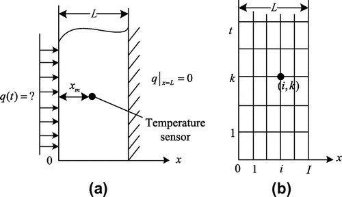
In Equation (1), T₀(x) is the initial temperature, q(t) is the surface heat flux, L is the thickness of slab, ρ denotes the constant density, $\mathit{\lambda }(T)$ and c_p(T) are the temperature-dependent thermal conductivity and specific heat, respectively.

The DHCP considered here represents the determination of the temperatures of the system of Equation (1), while the surface heat flux q(t) is given. In this work, the numerical method is used to solve the direct problem. Figure 1(b) shows the grid division of time and space. By applying the heat balance method [16] into Equation (1), the discretization equations of nodes can be derived(2a) $$\mathit{\rho }{c}_{p,0}^k\frac{T_0^{k+1}-T_0^k}{\mathrm{\Delta }t}=\left(q_k+\frac{T_1^{k+1}-T_0^{k+1}}{\mathrm{\Delta }{x}_1/2{\mathit{\lambda }}_1^k+\mathrm{\Delta }{x}_0/{\mathit{\lambda }}_0^k}\right)/\mathrm{\Delta }{x}_0,$$(2a) (2b) $$\mathit{\rho }{c}_{p,i}^k\frac{T_i^{k+1}-T_i^k}{\mathrm{\Delta }t}=\left(\frac{T_{i+1}^{k+1}-T_i^{k+1}}{\mathrm{\Delta }{x}_{i+1}/2{\mathit{\lambda }}_{i+1}^k+\mathrm{\Delta }{x}_i/2{\mathit{\lambda }}_i^k}+\frac{T_{i-1}^{k+1}-T_i^{k+1}}{\mathrm{\Delta }{x}_{i-1}/2{\mathit{\lambda }}_{i-1}^k+\mathrm{\Delta }{x}_i/2{\mathit{\lambda }}_i^k}\right)/\mathrm{\Delta }{x}_i\left(i=1,\dots ,I-1\right),$$(2b) (2c) $$\mathit{\rho }{c}_{p,I}^k\frac{T_I^{k+1}-T_I^k}{\mathrm{\Delta }t}=\left(\frac{T_{I-1}^{k+1}-T_I^{k+1}}{\mathrm{\Delta }{x}_{I-1}/2{\mathit{\lambda }}_{I-1}^k+\mathrm{\Delta }{x}_I/{\mathit{\lambda }}_I^k}\right)/\mathrm{\Delta }{x}_I$$(2c)

where $T_i^k=T(x_i,t_k)$, x_i = iΔx, t_k = kΔt, Δx = L/I, I denotes the number of nodes minus one, Δt is the time step size, Δx is the space step size; ${\mathit{\lambda }}_i^k$ and $c_{p,i}^k$ is the thermal conductivity and the specific heat capacity on the node (i, k), k = 0, 1, 2,… , K, i = 0, 1, 2,… , I. The temperatures of each nodes can be obtained by solving Equation (2) utilizing the tridiagonal matrix algorithm (TDMA) [16].

On the contrary, the IHCP is to estimate the unknown surface heat flux q(t) by utilizing the measured temperature at the temperature sensor location x_m.

3. Multi-model inverse method

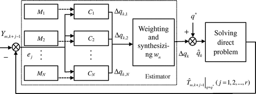
The multi-model inversion system structure is shown in Figure 2. In this figure, q^* is the initial guess surface heat flux, the symbol ${\left.{\widehat{T}}_{m,k+j-1}\right|}_{q=q^{\ast }}$ (j = 1, 2,… , r) represents the calculated temperature for the nonlinear direct problem at time t_k+j−1 and at the sensor location x_m for the initial guess surface heat flux q^*, r is the number of future time steps, Y_m,k+j−1(j = 1, 2,… , r) is the measured temperature at time t_k+j−1and at the sensor location x_m, Δq_k,n (n = 1, 2, …, N) is the output of the controller n, Δq_k is the total amount of current heat flux compensation, ${\widehat{q}}_k$ is the estimated heat flux, w_n is the weighting coefficient of model schedule. The dashed box denotes the multi-model estimator or controller.

Figure 2. Block scheme of the multi-model inversion system.

The nonlinear DHCP is approximated by N linear local models M_n (n = 1, 2, …, N). Each of the local models corresponds to a linear local controller C_n (n = 1, 2, …, N). The total output of the controller is obtained by weighting and synthesizing the outputs of the local controllers. Local models, local controllers and the model switching strategy will be described in detail later.

The multi-model inversion system works as follows: Assume an initial heat flux guess value of q^*, calculate the calculated temperature by performing the DHCP and calculate the error signal e_j,(3) $$e_j=Y_{m,k+j-1}-{\left.{\widehat{T}}_{m,k+j-1}\right|}_{q=q^{\ast }}(j=1,2,\dots ,r).$$(3)

Calculate the output $\mathrm{\Delta }{q}_{k,n}$ of the linear local controller C_n which corresponds to the linear local model M_n by inputting the error signal into the local controller. The total amount of current heat flux compensation is obtained by weighting and synthesizing the outputs of the local controllers, namely,(4) $$\mathrm{\Delta }{q}_k=\sum _{n=1}^N{w}_n\mathrm{\Delta }{q}_{k,n}.$$(4)

Eventually, the estimated current heat flux is(5) $${\widehat{q}}_k=q^{\ast }+\mathrm{\Delta }{q}_k,$$(5)

and repeat the process until the inverse process finishes.

There are some important points about this multi-model inverse method that should be noted here:

(1)	In the multi-model inversion, the local models are generally the linear models. Partial differential equations, ordinary differential equations, transfer functions, algebraic equations and the other linear models all can be used as the local models.
(2)	For the local controller, since the local model is a linear model, all excellent linear control algorithms or linear estimators can be used as the local controller.
(3)	The local model set has been determined before the inverse process begins, however, the existing nonlinear inverse methods are usually the adaptive method which determines the local models in real time. If N is equal to 1, the multi-model method becomes a simple linear single model method. If N tends to infinity, the multi-model method can tend to the nonlinear model. When N is the moderate value, the multi-model method not only possesses the sufficient approximate accuracy to the nonlinear model, but also ensures the adequate computational efficiency.
(4)	The model switching strategy is extremely important. It selects one or a few local models that can describe the controlled object as the most appropriate models. The designed controllers based on the most appropriate models are switched to the current controllers. Because the controlled object of the inversion is virtual device, i.e. the nonlinear heat conduction equations, we can select the typical temperature as the switching variable of the best model. Thus, the multi-model can represent the nonlinear model as accurately as possible.

Now, we take the nonlinear heat flux inverse problem for an example, and discuss the three components of the multi-model inverse method: local models, local controllers and the model switching strategy.

3.1. Local models

The establishment process of the local model set of the multi-model method has three steps:

(1)	Select the model switching variable v. The output, the input and the state variables of the controlled system are the typical choice. In this paper, the measured temperature Ym,k is chosen as the model switching variable, namely, v = Ym,k.
(2)	Suppose the model switching variable v ⊂ [vmin, vmax], and select N operating balance points in the operating interval of the switching variable. the operating balance points can be determined as follows:(6) $$v_{\text{b,}n}=v_{min}+(n-1)(v_{max}-v_{min})/(N-1)(n=1,2,\dots ,N).$$(6)
(3)	Establish the linear local models by linearizing the nonlinear model around balance points. In this paper, the governing equation of the linear local model Mn is(7) $$\mathit{\rho }{c}_p(v_{\text{b,}n})\frac{\mathit{\partial }T(x,t)}{\mathit{\partial }t}=\mathit{\lambda }(v_{\text{b,}n})\frac{{\mathit{\partial }}^{2}T(x,t)}{\mathit{\partial }{x}^2}(n=1,2,\dots ,N).$$(7)

The determination of the number of local models N depends on the nonlinearity degree of the actual object. It cannot be neither too much nor too less. Too much leads to low computational efficiency, while too less results in low calculating accuracy.

3.2. Local controllers

For the linear local models, any linear controller can be used in the multi-model inverse method. In order to illustrate the two advantages of the multi-model inverse method, namely, improving the computational efficiency and enlarging the applied range of the complicated linear controllers, we will employ the DMC [17–19] and DMC filter as the local controllers of the multi-model inverse method.

3.2.1. Prediction model

The aim of establishing the DMC prediction model is to predict the temperature T_m,k+j−1 (j = 1, 2, …, r) at the temperature sensor location x_m by the heat flux increments Δq_k, Δq_k+1, …, Δq_k+r−1 at times t_k, t_k+1, …, t_k+r−1.

Because all local models are linear. According to the superposition principle, when the heat flux increments Δq_k+j−1 (j = 1, 2, …, r) are input into the heat conduction system from time t_k, the output temperature T_m,k+j−1 at time t_k+j−1 and at the sensor location x_m is the sum of the output temperature ${\widehat{T}}_{m,k+j-1}$ at the time t_k+j−1 without any control actions and the output temperature(s) ΔT_m,k+j−1 due to the heat flux increment(s) Δq_k through Δq_k+j−1 inclusive, i.e.(8a) $$T_{m,k}={\left.{\widehat{T}}_{m,k}\right|}_{\mathrm{\Delta }{q}_k=0}+{\mathit{\varphi }}_m^0\mathrm{\Delta }{q}_k,$$(8a) (8b) $$T_{m,k+1}={\left.{\widehat{T}}_{m,k+1}\right|}_{\mathrm{\Delta }{q}_k=\mathrm{\Delta }{q}_{k+1}=0}+{\mathit{\varphi }}_m^1\mathrm{\Delta }{q}_k+{\mathit{\varphi }}_m^0\mathrm{\Delta }{q}_{k+1},$$(8b) (8c) $$T_{m,k+2}={\left.{\widehat{T}}_{m,k+2}\right|}_{\mathrm{\Delta }{q}_k=\mathrm{\Delta }{q}_{k+1}=\mathrm{\Delta }{q}_{k+2}=0}+{\mathit{\varphi }}_m^2\mathrm{\Delta }{q}_k+{\mathit{\varphi }}_m^1\mathrm{\Delta }{q}_{k+1}+{\mathit{\varphi }}_m^0\mathrm{\Delta }{q}_{k+2},$$(8c) $$⋮$$(8d) $$T_{m,k+r-1}={\left.{\widehat{T}}_{m,k+r-1}\right|}_{\mathrm{\Delta }{q}_k=\mathrm{\Delta }{q}_{k+1}=\cdots =\mathrm{\Delta }{q}_{k+r-1}=0}+{\mathit{\varphi }}_m^{r-1}\mathrm{\Delta }{q}_k+{\mathit{\varphi }}_m^{r-2}\mathrm{\Delta }{q}_{k+1}+\cdots +{\mathit{\varphi }}_m^0\mathrm{\Delta }{q}_{k+r-1}$$(8d)

where ${\mathit{\varphi }}_m^{j-1}$ is the coefficient of dynamic step response at the sensor location x_m.

Equation (8) also can be written in the matrix form:(9) $${\mathit{T}}_m=\mathit{A}\mathrm{\Delta }\mathit{q}+{\widehat{\mathit{T}}}_m\left|{}_{\mathrm{\Delta }\mathit{q}=\mathbf{0}}\right.$$(9)

where(10) $${\mathit{T}}_m={[T_{m,k},T_{m,k+1},\dots ,T_{m,k+r-1}]}^T,$$(10) (11) $${\widehat{\mathit{T}}}_m\left|{}_{\mathrm{\Delta }\mathit{q}=\mathbf{0}}\right.={[{\left.{\widehat{T}}_{m,k+1}\right|}_{\mathrm{\Delta }{q}_k=0},{\left.{\widehat{T}}_{m,k+1}\right|}_{\mathrm{\Delta }{q}_k=\mathrm{\Delta }{q}_{k+1}=0},\dots ,{\left.{\widehat{T}}_{m,k+r-1}\right|}_{\mathrm{\Delta }{q}_k=\mathrm{\Delta }{q}_{k+1}=\cdots =\mathrm{\Delta }{q}_{k+r-1}=0}]}^T,$$(11) (12) $$\mathrm{\Delta }\mathit{q}={[\mathrm{\Delta }{q}_k,\mathrm{\Delta }{q}_{k+1},\dots ,\mathrm{\Delta }{q}_{k+r-1}]}^T,$$(12) (13) $$\mathit{A}=\left[\begin{array}{ccccc}{\mathit{\varphi }}_m^0& 0& 0& \cdots & 0\\ {\mathit{\varphi }}_m^1& {\mathit{\varphi }}_m^0& 0& \cdots & 0\\ ⋮& ⋮& ⋮& & ⋮\\ {\mathit{\varphi }}_m^{r-1}& {\mathit{\varphi }}_m^{r-2}& {\mathit{\varphi }}_m^{r-3}& \cdots & {\mathit{\varphi }}_m^0\end{array}\right].$$(13)

The system dynamic step response model is used for the predictive model in DMC algorithm. The system step response function $Z(x,t)=\frac{\mathit{\partial }T(x,t)}{\mathit{\partial }{q}_k}$ is defined as the response degree of the temperature T(x, t) to the heat flux q_k. By differentiating Equation (7(7) $$\mathit{\rho }{c}_p(v_{\text{b,}n})\frac{\mathit{\partial }T(x,t)}{\mathit{\partial }t}=\mathit{\lambda }(v_{\text{b,}n})\frac{{\mathit{\partial }}^{2}T(x,t)}{\mathit{\partial }{x}^2}(n=1,2,\dots ,N).$$(7) ) with respect to q_k, the step response function Z(x, t) over the time interval $[t_k,t_{k+r-1}]$ should satisfy the following step response equations:(14a) $$\mathit{\rho }{c}_p(v_{\text{b,}n})\frac{\mathit{\partial }Z(x,t)}{\mathit{\partial }t}=\mathit{\lambda }(v_{\text{b,}n})\frac{{\mathit{\partial }}^{2}Z(x,t)}{\mathit{\partial }{x}^2}(n=1,2,\dots ,N),$$(14a) (14b) $$Z(x,t_{k-1})=0,$$(14b) (14c) $$-\mathit{\lambda }(v_{\text{b,}n})\frac{\mathit{\partial }Z(x,t)}{\mathit{\partial }x}\left|{}_{x=0}\right.=1,$$(14c) (14d) $$-\mathit{\lambda }(v_{\text{b,}n})\frac{\mathit{\partial }Z(x,t)}{\mathit{\partial }x}\left|{}_{x=L}\right.=0.$$(14d)

Notice that it is not necessary to know $q_k$, $q(t)$, or even T_k−1(x) to obtain the solution for the step response function $Z(x,t)$, because Equation (14) is not the function of $q_k$, $q(t)$, or T_k−1(x). Equation (14) can be solved by the aforementioned heat balance method and TDMA [16], and the numerical solution $Z_m^{k+j-1}(j=1,2,\dots ,r)$ of the step response function is obtained. Finally, the dynamic step response coefficients at the sensor location x_m are determined by:(15) $${\mathit{\varphi }}_m^{j-1}=Z_m^{k+j-1}(j=1,2,\dots ,r).$$(15)

3.2.2. Rolling optimization

In order to estimate the heat flux increments, the optimization objective function to be minimized is defined as(16) $$minJ(\mathrm{\Delta }{q}_k,\mathrm{\Delta }{q}_{k+1},\dots ,\mathrm{\Delta }{q}_{k+r-1})=\sum _{j=1}^r(Y_{m,k+j-1}-T_{m,k+j-1}{)}^2+\mathit{\alpha }\sum _{j=1}^r{(\mathrm{\Delta }{q}_{k+j-1})}^2$$(16)

where α is the regularization parameter. The first term in the optimization objective function (16) is the fidelity of the estimator with the measured temperature data, while the second term expresses the regularity (or smoothness) required from the unknown heat flux.

Equation (16(16) $$minJ(\mathrm{\Delta }{q}_k,\mathrm{\Delta }{q}_{k+1},\dots ,\mathrm{\Delta }{q}_{k+r-1})=\sum _{j=1}^r(Y_{m,k+j-1}-T_{m,k+j-1}{)}^2+\mathit{\alpha }\sum _{j=1}^r{(\mathrm{\Delta }{q}_{k+j-1})}^2$$(16) ) can be written in the matrix form:(17) $$minJ(\mathrm{\Delta }\mathit{q})={({\mathit{Y}}_m-{\mathit{T}}_m)}^T\text{(}{\mathit{Y}}_m-{\mathit{T}}_m)+\mathit{\alpha }\mathrm{\Delta }{\mathit{q}}^T\mathrm{\Delta }\mathit{q}$$(17)

where(18) $${\mathit{Y}}_m={[Y_{m,k},Y_{m,k+1},\dots ,Y_{m,k+r-1}]}^T.$$(18)

Substituting Equation (9(9) $${\mathit{T}}_m=\mathit{A}\mathrm{\Delta }\mathit{q}+{\widehat{\mathit{T}}}_m\left|{}_{\mathrm{\Delta }\mathit{q}=\mathbf{0}}\right.$$(9) ) into Equation (17(17) $$minJ(\mathrm{\Delta }\mathit{q})={({\mathit{Y}}_m-{\mathit{T}}_m)}^T\text{(}{\mathit{Y}}_m-{\mathit{T}}_m)+\mathit{\alpha }\mathrm{\Delta }{\mathit{q}}^T\mathrm{\Delta }\mathit{q}$$(17) ), differentiating the Equation (17(17) $$minJ(\mathrm{\Delta }\mathit{q})={({\mathit{Y}}_m-{\mathit{T}}_m)}^T\text{(}{\mathit{Y}}_m-{\mathit{T}}_m)+\mathit{\alpha }\mathrm{\Delta }{\mathit{q}}^T\mathrm{\Delta }\mathit{q}$$(17) ) with respect to the vector $\mathrm{\Delta }\mathit{q}$, setting the resulting equation equal to zero, the optimal control increment vector $\mathrm{\Delta }\mathit{q}$ can be obtained as follows:(19) $$\mathrm{\Delta }\mathit{q}={({\mathit{A}}^T\mathit{A}+\mathit{\alpha }\mathit{I})}^{-1}{\mathit{A}}^T\left({\mathit{Y}}_m-{\widehat{\mathit{T}}}_{\mathit{m}}\left|{}_{\mathrm{\Delta }\mathit{q}=\mathbf{0}}\right.\right).$$(19)

It is emphasized that only the current heat flux increment Δq_k is required to estimate the heat flux in the DMC algorithm. At the next moment, Δq_k+1 is obtained by the same optimization method, and this is the ‘rolling optimization’ strategy. The optimal value of the heat flux by Equation (19(19) $$\mathrm{\Delta }\mathit{q}={({\mathit{A}}^T\mathit{A}+\mathit{\alpha }\mathit{I})}^{-1}{\mathit{A}}^T\left({\mathit{Y}}_m-{\widehat{\mathit{T}}}_{\mathit{m}}\left|{}_{\mathrm{\Delta }\mathit{q}=\mathbf{0}}\right.\right).$$(19) ) is(20) $${\widehat{q}}_k=[1,0,\dots ,0]{({\mathit{A}}^T\mathit{A}+\mathit{\alpha }\mathit{I})}^{-1}{\mathit{A}}^T\left({\mathit{Y}}_m-{\widehat{\mathit{T}}}_{\mathit{m}}\left|{}_{\mathrm{\Delta }\mathit{q}=\mathbf{0}}\right.\right).$$(20)

3.2.3. DMC digital filter

Digital filters possess advantages in high computational efficiency, near real-time nature, easy implementation and so on [8,15]. Unfortunately, the digital filter can only be applied to the linear problems, and there is no effective way for the nonlinear problems. In this article, we propose to take the advantages of the multi-model method to solve the nonlinear inverse problems by the DMC digital filter.

Each linear controller can be rewritten as a digital filter by the linear characteristics of the problems [8]. DMC digital filter can be expressed as a linear combination of $k_{\text{p}}$ past measured temperatures and $k_{\text{f}}$ future measured temperatures, i.e.(21) $$\mathrm{\Delta }{q}_k=\sum _{j=0}^{k_{\text{f}}+k_{\text{p}}}{f}_{k_{\text{f}}+k_{\text{p}}-j}\left(Y_{m,k-k_{\text{p}}+j}-{\left.{\widehat{T}}_{m,k-k_{\text{p}}+j}\right|}_{q=q^{\ast }}\right)$$(21)

where f is the filter coefficient, $Y_{m,k-k_{\text{p}}+j}$ is the measured temperature, q^* is the initial guess surface heat flux, ${\left.{\widehat{T}}_{m,k-k_{\text{p}}+j}\right|}_{q=q^{\ast }}$ represents the calculated temperature for the nonlinear direct problem at time $t_{k-k_{\text{p}}+j}$ and at the sensor location x_m for the initial guess surface heat flux q^*.

In order to calculate the DMC digital filter coefficients, set $k_{\text{f}}=r$, and (22) $$\begin{array}{c}{Y}_{m,r}-{\left.{\widehat{T}}_{m,r}\right|}_{q=q^{\ast }}=1,\\ Y_{m,j}-{\left.{\widehat{T}}_{m,j}\right|}_{q=q^{\ast }}=0,\text{for}j\ne r\end{array}.$$(22)

Sequentially using the DMC inverse algorithm Equation (20(20) $${\widehat{q}}_k=[1,0,\dots ,0]{({\mathit{A}}^T\mathit{A}+\mathit{\alpha }\mathit{I})}^{-1}{\mathit{A}}^T\left({\mathit{Y}}_m-{\widehat{\mathit{T}}}_{\mathit{m}}\left|{}_{\mathrm{\Delta }\mathit{q}=\mathbf{0}}\right.\right).$$(20) ) with Equation (22(22) $$\begin{array}{c}{Y}_{m,r}-{\left.{\widehat{T}}_{m,r}\right|}_{q=q^{\ast }}=1,\\ Y_{m,j}-{\left.{\widehat{T}}_{m,j}\right|}_{q=q^{\ast }}=0,\text{for}j\ne r\end{array}.$$(22) ), we can obtain each DMC digital filter coefficient, namely,(23) $$f_{k-1}={\widehat{q}}_k\left|{}_{\begin{array}{c}{Y}_{m,r}-{\left.{\widehat{T}}_{m,r}\right|}_{q=q^{\ast }}=1,\hfill \\ Y_{m,j}-{\left.{\widehat{T}}_{m,j}\right|}_{q=q^{\ast }}=0,\text{for}j\ne r\hfill \end{array}}\right.,k=1,2,\dots ,k_{\text{f}}+k_{\text{p}}+1.$$(23)

Because the formula of filter coefficients is extremely complicated, it is almost impossible to adaptively solve the filter coefficients for the nonlinear problems step by step in a near real time manner. However, we can successfully apply linear digital filters to nonlinear problems by taking the advantage of multi-model inverse method which can obtain filter coefficients beforehand. As our attentions are focused on the multi-model inverse method, for the DMC digital filter, the interested reader is referred to [8,15] for details.

3.3. Model switching strategy

The model switching strategy is to select one or a few local models that can describe the controlled object as the most appropriate models. Based on the matching degree between local models and the current inverse model, the weighting coefficients of the local controllers to the local models are determined. The total amount of current heat flux compensation is the weighted average of all local controller outputs, namely,(24) $$\mathrm{\Delta }{q}_k=\sum _{n=1}^N{w}_n\mathrm{\Delta }{q}_{k,n}.$$(24)

The weighting coefficient w_n is established as follows:(25) $$w_n=\frac{exp\left(-\left|v_{\text{b,}n}-Y_{m,k}\right|\right)}{{\sum }_{n=1}^{N}exp\left(-\left|v_{\text{b,}n}-Y_{m,k}\right|\right)}$$(25)

where the single bars are absolute value sign. It can be shown that the weighting coefficients sum to unity:(26) $$\sum _{n=1}^N{w}_n=1.$$(26)

3.4. The computational procedure of the inverse estimation

The computational procedure of the aforementioned multi-model inverse method can be summarized as follows:

(1)	Select N operating balance points $v_{\text{b,}n}$ (n = 1, 2,… , N) in the operating interval of the switching variable.
(2)	Establish N linear local models Mn (n = 1, 2,… , N) by linearizing the nonlinear model around operating balance points.
(3)	Assume an initial heat flux guess value of q* and set k = 1.
(4)	Solve the DHCP to obtain the calculated temperature and calculate the error signal by Equation (3(3) $$e_j=Y_{m,k+j-1}-{\left.{\widehat{T}}_{m,k+j-1}\right|}_{q=q^{\ast }}(j=1,2,\dots ,r).$$(3) ).
(5)	Calculate the output $\mathrm{\Delta }{q}_{k,n}$ of the linear local controller Cn (n = 1, 2,… , N) which corresponds to the linear local model Mn by Equation (20(20) $${\widehat{q}}_k=[1,0,\dots ,0]{({\mathit{A}}^T\mathit{A}+\mathit{\alpha }\mathit{I})}^{-1}{\mathit{A}}^T\left({\mathit{Y}}_m-{\widehat{\mathit{T}}}_{\mathit{m}}\left|{}_{\mathrm{\Delta }\mathit{q}=\mathbf{0}}\right.\right).$$(20) ) or Equation (21(21) $$\mathrm{\Delta }{q}_k=\sum _{j=0}^{k_{\text{f}}+k_{\text{p}}}{f}_{k_{\text{f}}+k_{\text{p}}-j}\left(Y_{m,k-k_{\text{p}}+j}-{\left.{\widehat{T}}_{m,k-k_{\text{p}}+j}\right|}_{q=q^{\ast }}\right)$$(21) ).
(6)	Calculate the total amount of current heat flux compensation by weighting and synthesizing the outputs of the local controllers.
(7)	Compute the newest estimated heat flux ${\widehat{q}}_k$by Equation (5(5) $${\widehat{q}}_k=q^{\ast }+\mathrm{\Delta }{q}_k,$$(5) ).
(8)	Set k = k + 1, and return to step 4.

4. Numerical tests and discussions

4.1. The conditions of simulation experiments

In order to verify the feasibility and effectiveness of the multi-model inverse method, we have discussed a one-dimensional nonlinear transient inverse problem in Section 2 through numerical experiments. In each test case, L = 0.05 m, T₀ = 300 K, Δt = 0.6 s, I = 20, x_m = 1.25 × 10⁻² m. Given slab is Armco iron, and its temperature-dependent thermal properties are taken from the literature [20] and shown in Table 1. The thermal conductivity and specific heat are considered piecewise linear functions of temperature. The surface heat flux history is assumed as the following rectangular pulse variation function:(27) $$q=\left\{\begin{array}{cc}1600{\text{kW m}}^{-2},\hfill & \text{for}30\le t\le 90\text{s};\hfill \\ 0,\hfill & \text{elsewhere}.\hfill \end{array}\right.$$(27)

Table 1. Thermal properties of Armco (99.75% pure) [20].

Temperature (K)	Thermal conductivity (W m^−1 K^−1)	Specific heat (J kg^−1 K^−1)	Density (kg m^−3)
200	80.6	384	7870
400	65.7	490	7870
600	53.1	574	7870
800	42.2	680	7870
1000	32.3	975	7870
1200	28.7	609	7870
1500	31.4	654	7870

In this paper, all numerical tests are implemented in a Dell^® computer with 2.00 GHz Intel Pentium® dual CPU and 2 GB RAM. The computer programs are coded by the MATLAB R2013a.

In the practical engineering, measurement errors inevitably exist in the measured temperatures. The measured temperatures are gained by the following formula:(28) $$Y_{m,k}={(T_{m,k})}_{\text{exa}}+\mathit{\omega }\mathit{\sigma }$$(28)

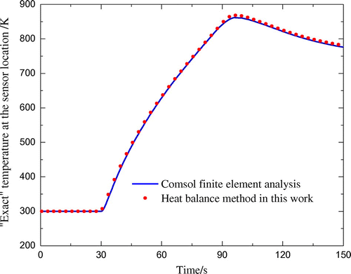
where σ is the standard deviation of the measurement errors, and ω is a random variable of the standard normal distribution with zero mean and unit standard deviation in the confidence interval [2.576, 2.576] for a 99% confidence coefficient. The exact temperature ${(T_{m,k})}_{\text{exa}}$ can be obtained by solving the direct problem with the ‘exact’ heat flux Equation (27(27) $$q=\left\{\begin{array}{cc}1600{\text{kW m}}^{-2},\hfill & \text{for}30\le t\le 90\text{s};\hfill \\ 0,\hfill & \text{elsewhere}.\hfill \end{array}\right.$$(27) ) and shown in Figure 3.

Figure 3. Comparison of temperature evolution calculated by the heat balance method in this work and the finite element software Comsol.

In this paper, the regularization parameter in DMC is determined according to the discrepancy principle [18,19].

In order to validate the validity of the direct problem solution in this paper, the temperature evolution at the sensor location calculated by the heat balance method in this work is compared with the analysis result by the commercial finite element software Comsol. The consistency of the results of the two methods (Figure 3) demonstrates the validity of the direct problem solution in this paper.

In order to measure the errors, the root mean square error of the estimated heat flux is introduced and defined as follows:(29) $$S_{\text{q}}={\left[\frac{1}{K-1}\sum _{k=1}^K{\left({\widehat{q}}_k-q_k\right)}^2\right]}^{1/2}.$$(29)

4.2. Multi-model inverse method based on DMC

4.2.1. Effect of the number of local models on the inversion results

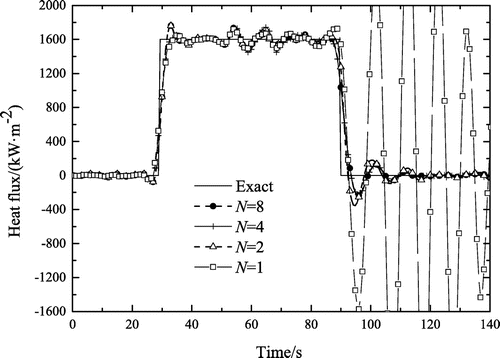
Set $\mathit{\sigma }=0.5$ K, r = 10, $\mathit{\alpha }=1\times {10}^{-10}$ K² m⁴ W⁻². To investigate the effect of the number of local models on the accuracy and computational efficiency of the multi-model method, the number of local models N is 1, 2, 4 and 8, respectively, and their corresponding sets of balance points are listed in column two of Table 2. Table 2 provides details of the test results. The root mean square error of the estimated heat flux S_q expresses the inversion accuracy. The smaller its value, the more accurate the inversion result. It can be seen from Table 2 that when the number of local models N increases, the estimated heat flux is more accurate, but the computation time becomes longer. Figure 4 shows the inversion results of the multi-model method with different numbers of local models. From Figure 4 and Table 2, we can conclude that when N is greater than 4, the number of local models has little effect on the improvement of the inversion accuracy, but it increases the computation time. Hence, the number of local models is set equal to 4 in the following numerical simulation tests.

Table 2. Effect of the number of local models on the inversion results.

Number of local models	Set of balance points /K	Computation time/s	Sq/(W m^−2)
N = 1	{600}	3.04	1.00 × 10^6
N = 2	{500, 900}	3.27	1.30 × 10^5
N = 4	{300, 500, 700, 900}	3.35	1.23 × 10^5
N = 8	{200, 300, 400, 500, 600, 700, 800, 900}	3.53	1.22 × 10^5

Figure 4. Inversion results of the multi-model method with different numbers of local models.

4.2.2. Comparison of the single model, adaptive model and multi-model method

Set $\mathit{\sigma }=0.5$ K, r = 10, $\mathit{\alpha }=1\times {10}^{-10}$ K² m⁴ W⁻². The balance point sets of the single model and multi-model method are shown in Table 3. The adaptive model method obtains the models in each sampling time by finite difference method [8]. Table 3 gives the computation time and inversion accuracy of the single model, adaptive model and multi-model method. Figure 5 shows the corresponding inversion results of the single model, adaptive model and multi-model method. As can be seen from Table 3 and Figure 5, the inversion accuracy of the multi-model method is comparable to that of the adaptive model method, which is slightly better than the former. The single model method is the worst. The main reason of the different inversion accuracy for different methods is the different approximate accuracy of the prediction models. The adaptive model method approximates the inversion object by the linearization at each sampling time step. It approaches the approximation of infinite linear models, while the multi-model method approximates the inversion object by several typical linear prediction models. Hence, the inversion result of the adaptive model method is the most accuracy. The multi-model method is slightly worse than the adaptive model method. The single model method approximates the inversion object by only one typical linear prediction models, so the approximation is not exact and the estimated heat flux diverges. It also can be seen from Table 3 that the computation time of the adaptive model method requires about twice longer than that of the multi-model method, whose computation time is almost equal to that of the single model method. From the above numerical tests, we can arrive at the conclusion that the multi-model inverse method is a computationally efficient and accurate algorithm. So the multi-model inverse method is a worthy recommended algorithm in the practical applications.

Table 3. Comparison of the single model, adaptive model and multi-model method.

Inverse method	Set of balance points/K	Computation time/s	Sq/(W m^−2)
Single model	{600}	3.04	1.00 × 10^6
Multi-model	{300, 500, 700, 900}	3.35	1.23 × 10^5
Adaptive model	–	6.42	1.20 × 10^5

Figure 5. Comparison of the single model, adaptive model and multi-model method.

4.3. Multi-model inverse method based on DMC digital filter

4.3.1. DMC digital filter coefficients

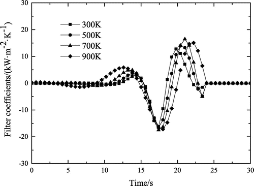
Set $\mathit{\alpha }=1\times {10}^{-10}$ K² m⁴ W⁻², k_p = 30, k_f = r = 10. The balance point set is {300, 500, 700, 900} K. The measured temperatures are given as Equation (22(22) $$\begin{array}{c}{Y}_{m,r}-{\left.{\widehat{T}}_{m,r}\right|}_{q=q^{\ast }}=1,\\ Y_{m,j}-{\left.{\widehat{T}}_{m,j}\right|}_{q=q^{\ast }}=0,\text{for}j\ne r\end{array}.$$(22) ). Figure 6 shows the DMC digital filter coefficients at different balance point temperatures. In Figure 6, the unit measured temperature impulse occurs at time t_k = 18 s. As shown in Figure 6, with the balance point temperature decreasing, the filter coefficients approach to the moment t_k = 18 s, at which the unit measured temperature impulse occurs. This phenomenon mainly results from the temperature-dependent characteristics of the material thermal properties. The thermal diffusivity of the material is 2.13 × 10⁻⁵ m² s⁻¹ at 300 K, while it is 5.72 × 10⁻⁶ m² s⁻¹ at 900 K. When the thermal diffusivity of the material is large, the thermal inertia of the heat conduction system is small. Due to the great difference of the filter coefficients at different temperatures, employing the single model method may lead to large inverse error, while using the adaptive model method may result in the difficulty of implementation, because the filters coefficients almost cannot be calculated in near real time manner. Using the multi-model method can effectively solve this nonlinear problem, because all linear local models are calculated beforehand.

Figure 6. DMC digital filter coefficients at different balance point temperatures ($\mathit{\alpha }=1\times {10}^{-10}$ K² m⁴ W⁻², k_p = 30, k_f = 10, t_k = 18 s).

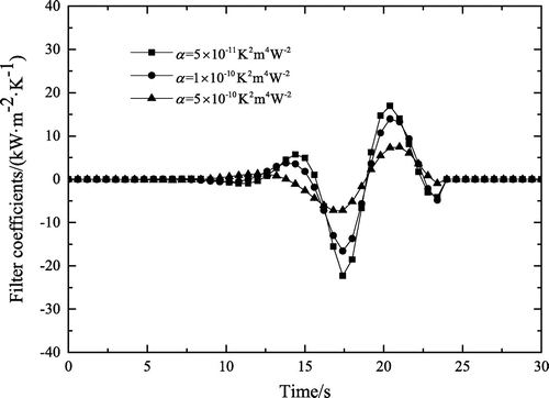
Set k_p = 30, k_f = r = 10, t_k = 18 s, $v_{\text{b,}n}$ = 600 K. Figure 7 shows the DMC digital filter coefficients for α = 5 × 10⁻¹⁰, 1 × 10⁻¹⁰ and 5 × 10⁻¹¹ K² m⁴ W⁻². It can be seen that the filter coefficients are sensitive to the choice of the regularization parameter. The larger the regularization parameter is, the flatter the curve of filter coefficients is, and the smaller the absolute values of filter coefficients are. If the regularization parameter is large, the random error of the estimated heat flux is small.

Figure 7. The DMC digital filter coefficients for α = 5 × 10⁻¹⁰, 1 × 10⁻¹⁰ and 5 × 10⁻¹¹ K² m⁴ W⁻² (k_p = 30, k_f = 10, t_k = 18 s, $v_{\text{b,}n}$ = 600 K).

For the example in this article, an important characteristic of filter coefficients is that the sum of filter coefficients is equal to zero. Applying Equation (21(21) $$\mathrm{\Delta }{q}_k=\sum _{j=0}^{k_{\text{f}}+k_{\text{p}}}{f}_{k_{\text{f}}+k_{\text{p}}-j}\left(Y_{m,k-k_{\text{p}}+j}-{\left.{\widehat{T}}_{m,k-k_{\text{p}}+j}\right|}_{q=q^{\ast }}\right)$$(21) ) to the steady-state heat conduction in Section 2, we have ${\widehat{q}}_k=\left.({\sum }_{i=0}^{k_{\text{f}}+k_{\text{p}}}{f}_{k_{\text{f}}+k_{\text{p}}-i}\right)\left[Y_{m,k-k_{\text{p}}+i}-{\left.{\widehat{T}}_{m,k-k_{\text{p}}+i}\right|}_{q=0}\right]=0$. For different conditions, $Y_{m,k-k_{\text{p}}+i}-{\left.{\widehat{T}}_{m,k-k_{\text{p}}+i}\right|}_{q=0}$ can be arbitrary constant, so ${\sum }_{i=0}^{k_{\text{f}}+k_{\text{p}}}{f}_{k_{\text{f}}+k_{\text{p}}-i}=0$. Notice that the sum of the filter coefficients is not always equal to zero for all conditions.

4.3.2. Effect of the initial guess value of the surface heat flux on the inversion results

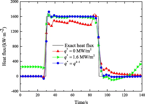
Set $\mathit{\sigma }=0$ K, $\mathit{\alpha }=1\times {10}^{-10}$ K² m⁴ W⁻², k_p = 20, k_f = r = 10, $v_{\text{b,}n}$ = {300, 500, 700, 900} K. Results of the estimated surface heat flux by DMC filter are shown in Figure 8 for different initial guess values of the surface heat flux $q^{\ast }=q^{k-1}$, $q^{\ast }=0$ MW m⁻² and $q^{\ast }=1.6$ MW m⁻². It is clear that the result of $q^{\ast }=q^{k-1}$ is superior to that of $q^{\ast }=0$ MW m⁻² and $q^{\ast }=1.6$MW m⁻². This mainly results from the nonlinear characteristic of the inversion object. The DMC filter needs to calculate k_p + k_f calculated temperatures, $T_{m,k_{\text{f}}+k_{\text{p}}-j}(q^{\ast })$. The time span is $(k_{\text{f}}+k_{\text{p}}+1)\mathrm{\Delta }t$ and very long. In nonlinear case, there is a great difference in the calculated temperatures for different initial guess values of the heat flux. The appropriate initial guess value of heat flux would improve the inversion accuracy. Hence we recommend $q^{\ast }=q^{k-1}$.

Figure 8. Effect of the initial guess value of the surface heat flux on the inversion results by DMC filter. ($\mathit{\alpha }=1\times {10}^{-10}$ K² m⁴ W⁻²)

4.3.3. Multi-model inverse method based on DMC filter

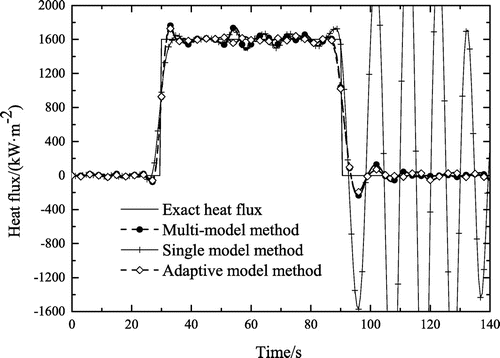
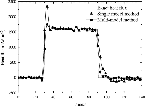
Comparison of the estimated surface heat flux by multi-model and single model method associated with DMC digital filter with noisy-free measured temperature is shown in Figure 9. In Figure 9, the balance point set of the multi-model method is {300, 500, 700, 900} K, while the single model method uses the thermal properties at 600 K. The estimated heat flux by the multi-model inverse method is significantly superior to that by the single model method. In the first step stage, the multi-model method has smaller overshoot than the single model method, while in the second step stage the setting time of the single model method is longer than that of multi-model method. The main reason of this phenomenon is the strong mismatch between the prediction model and the inversion object or the controlled object. In the inverse problems, we always assume that the inversion object perfectly matches the controlled object. By using the multi-model method, the degree of the match between the prediction model and the inversion object or the controlled object can be improved, therefore, the inversion result is more accurate.

Figure 9. Comparison of the inversion results of multi-model and single model method associated with DMC digital filter with noisy-free measured temperature. ($\mathit{\alpha }=1\times {10}^{-10}$ K² m⁴ W⁻², k_p = 20, k_f = r = 10).

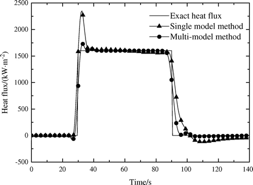
Comparison of the estimated surface heat flux by multi-model and single model method associated with DMC digital filter with $\mathit{\sigma }=0.5$ K is shown in Figure 10. It can be seen that the estimated heat flux by the multi-model inverse method is significantly superior to that by the single model method. Compared with Figure 10, due to the random measured temperature errors, slight fluctuation emerges, but the inversion result can satisfy the engineering application. It is also proved that the multi-model inverse method is a powerful algorithm for nonlinear problems.

Figure 10. Comparison of the inversion results of multi-model and single model method associated with DMC digital filter with $\mathit{\sigma }=0.5$ K. ($\mathit{\alpha }=1\times {10}^{-10}$ K² m⁴ W⁻², k_p = 20, k_f = r = 10).

5. Conclusions

The multi-model inverse method for nonlinear inverse problems is proposed based on multi-model control theory. The multi-model inverse method consists of three parts: local models, local controllers (or estimators), the model switching strategy. Some numerical tests are investigated to solve the one-dimensional nonlinear IHCP by the multi-model inverse method with the DMC and DMC filter being the local controllers, respectively.

Numerical tests of multi-model inverse method associated with DMC demonstrate that the multi-model inverse method is a highly computationally efficient and accurate algorithm by comparing with the single model and adaptive model method and that the multi-model inverse method is a worthy recommended inverse method in the practical applications.

Numerical tests of multi-model inverse method associated with DMC filter show that the multi-model method can extend the applied field of the complicated linear inverse algorithms such as digital filter to the nonlinear inverse problems and it can obtain satisfactory inversion results.

The multi-model inverse method can be extended to other complicated geometries and problems. The model switching strategy and the establishment of the linear local models need to be studied further.

Nomenclature
A	=	matrix of dynamic step response coefficients
cp	=	specific heat, J kg−1 K−1
e	=	error signal, K
fj	=	DMC digital filter coefficient, W m−2 K−1
I	=	number of spatial nodes
I	=	identity matrix
K	=	number of time nodes
L	=	slab thickness, m
mf	=	number of future time steps
mp	=	number of past time steps
N	=	number of local models
q	=	heat flux, W m−2
${\widehat{q}}_k$	=	estimated heat flux, W m−2
q*	=	initial guess surface heat flux, W m−2
r	=	number of future time steps
$S_{\text{q}}$	=	root mean square errors of the estimated heat flux, W m−2
t	=	time, s
T	=	temperature, K
T	=	vector of predicted temperatures
T0	=	initial temperature, K
${\left.\widehat{T}\right|}_{q=q^{\ast }}$	=	estimated temperatures for q = q*, K
${\widehat{\mathit{T}}}_m\left|{}_{\mathrm{\Delta }\mathit{q}=\mathbf{0}}\right.$	=	vector of estimated temperatures for $\mathrm{\Delta }\mathit{q}=\mathbf{0}$
w	=	weighting coefficient of model schedule
x	=	spatial coordinate, m
Y	=	measured temperature, K
Y	=	measured temperature vector
Z	=	dynamic step response coefficient, K m2 W−1

Greek symbols

α	=	regularization parameter, K2 m4 W−2
ϕ	=	coefficient of dynamic step response, K m2 W−1
Δt	=	sampling time step, s
Δx	=	spatial grid size, m
Δq	=	heat flux increments, W m−2
$\mathrm{\Delta }\mathit{q}$	=	vector of heat flux increments
λ	=	thermal conductivity, W m−1 K−1)
v	=	model switching variable
ρ	=	density, kg m−3
σ	=	standard deviation of the measurement error, K
ω	=	random variable

Subscripts/Superscripts

b	=	operating balance point
exa	=	exact temperature
i	=	spatial index
k	=	time index
m	=	temperature sensor location index
n	=	local model index

Disclosure statement

No potential conflict of interest was reported by the authors.

Funding

This work was supported by the National Natural Science Foundation of China [grant number 51676019].

References

- [cited 2017 Jan 3]. Available from: http://www.inverseproblems.org/index.html
- Hadamard J. Lectures on the Cauchy problem in linear partial differential equations. New Haven (CT): Yale University Press; 1923.
- Alifanov OM. Inverse heat transfer problems. Berlin: Springer-Verlag; 1994.10.1007/978-3-642-76436-3
- Ozisik MN, Orlande HRB. Inverse heat transfer fundamentals and application. New York (NY): Taylor and Francis; 2000.
- Woodbury KA. Inverse engineering handbook. Boca Raton (FL): CRC Press; 2002.10.1201/CRCHBKMECENG
- Orlande HRB, Fudym O, Maillet D, et al. Thermal measurements and inverse techniques. Boca Raton (FL): CRC Press; 2011.
- Tikhonov AN, Arsenin VY. Solutions of ill-posed problems. New York (NY): Wiley; 1977.
- Beck JV, Blackwell BF, Clair CRS Jr. Inverse heat conduction ill-posed problems. New York (NY): Wiley; 1985.
- Beck JV. Nonlinear estimation applied to the nonlinear inverse heat conduction problem. Int J Heat Mass Transf. 1970;13:703–716.10.1016/0017-9310(70)90044-X
- Beck JV, Litkouhi B, Clair CRS Jr. Efficient sequential solution of the nonlinear inverse heat conduction problem. Numer Heat Transf. 1982;5:275–286.
- Samadi F, Kowsary F, Sarchami A. Estimation of heat flux imposed on the rake face of a cutting tool: a nonlinear, complex geometry inverse heat conduction case study. Int Commun Heat Mass Transf. 2012;39:298–303.10.1016/j.icheatmasstransfer.2011.10.007
- Mohammadiun M, Molavi H, Bahrami HRT, et al. Application of sequential function specification method in heat flux monitoring of receding solid surfaces. Heat Transf Eng. 2013;35:933–941.
- Wang Z, Yao M, Wang X, et al. Inverse problem-coupled heat transfer model for steel continuous casting. J Mater Process Technol. 2014;214:44–49.10.1016/j.jmatprotec.2013.07.017
- Zhang LH, Tai BL, Wang GJ, et al. Thermal model to investigate the temperature in bone grinding for skull base neurosurgery. Med Eng Phys. 2013;35:1391–1398.10.1016/j.medengphy.2013.03.023
- Beck JV. Filter solutions for the nonlinear inverse heat conduction problem. Inv Probl Sci Eng. 2008;16:3–20.10.1080/17415970701198332
- Holman JP. Heat transfer. 10th ed. Boston (MA): McGraw-Hill Higher Education; 2010.
- Cutler CR, Ramakar BL. Dynamic matrix control – computer control algorithm. Proceedings of the Joint Automatic Control Conference, San Francisco (CA); 1980.
- Li Y, Wang G, Chen H. Simultaneously regular inversion of unsteady heating boundary conditions based on dynamic matrix control. Int J Therm Sci. 2015;88:148–157.10.1016/j.ijthermalsci.2014.09.013
- Li Y, Wang G, Chen H. Simultaneously estimation for surface heat fluxes of steel slab in a reheating furnace based on DMC predictive control. Appl Therm Eng. 2015;80:396–403.10.1016/j.applthermaleng.2015.01.069
- Incropera FP, Dewitt DP, Bergles TL, et al. Fundamentals of heat and mass transfer. 6th ed. Hoboken (NJ): Wiley; 2007.