A statistical approach to estimate state variables in flow-accelerated corrosion problems

Abstract

Sequential Monte Carlo or Particle Filter Methods have been widely used to deal with sequential Bayesian inference problems in several fields of knowledge. This technique involves approximation of probability sequences distributions of interest, by means of a large set of random samples, i.e. particles that are propagated along time with a simple Sampling Importance distribution, SI. A re-sampling technique is also used to improve the predictive probability. In this study, a methodology is proposed: apply the Bayesian filters to a state estimation problem involving the corrosion amount-time in a contraction–expansion geometry with the aid of Computational Fluid Dynamics to improve the accuracy of the results. The following filters were applied and compared: Sampling Importance Re-sampling filter (SIR filter) and Auxiliary Sampling Importance Re-sampling filter (ASIR filter). The corrosion model adopted is based on a double resistance due to the oxygen diffusion towards the wall through the hydrodynamic boundary layer and the oxide layer. Mass loss data over time are obtained from the literature to compare corrosion rates. Also, the influence of the corrosion products in rates of corrosion is discussed . Best results in corrosion damage estimation were obtained using the ASIR filter.

Keywords:

• Flow-accelerated corrosion
• SIR filter
• ASIR filter
• corrosion products
• double resistance model

AMS Subject Classifications:

• 60J60
• 80A23
• 82C80

1. Introduction

The corrosion of a material is defined as the deterioration of a material, generally a metallic one, by a chemical or electrochemical reaction. This deterioration can cause undesirable and harmful effects, including the mass loss of the base material. This phenomenon is, generally, a spontaneous process in which the reaction occurs continuously, transforming the material in such a way that the loss of durability and performance incapacitates the correct application for which it has been designed. One of the most important problems concerning the piping system is the wall mass loss caused by the transport of corrosive fluids. In turn, they induce the dissolution of an oxide layer on the inside wall that, progressively, reduces wall thickness to the point of failure. Also, the dissolution mechanism is related to the fluid flow regimes (mainly turbulent flows) especially near to the components like elbows, orifices and valves.

Within many flow systems, such as carbon steel corrosion, the increase in flow velocity leads to an increase in the corrosion rate. In this case, to verify how the dissolution of mass transfer controlled mechanism will contribute to the corrosion rate; or how the transport of oxygen was from the solutions bulk to the metal surface, Mahato et al. [1–3] have proposed a qualitative description of velocity and concentration distributions and effect of surface roughness in turbulent flow. According to these authors, the turbulent boundary layer thickness comprises a laminar sublayer thickness. Then, this laminar sublayer comprises a diffusion sublayer which forms the main resistance to mass transfer.

As corrosion proceeds, there is a continuous evolution of corrosion products that layer with time on the inner wall. Since this phenomenon in itself follows a complex and not fully understood mechanism, the qualitative portrayal proposed by Mahato [3], that is still valid and useful in many recent researches [4–7], indicates that the corrosion process consists of four steps: – diffusion of ${\text{O}}_2$ to the solid-liquid interface through a viscous sublayer; – diffusion of dissolved ${\text{O}}_2$ through the layer of corrosion products; – reaction at the surface; and, – precipitation of corrosion products at the solid surface. According to Mahato [3] as the corrosion product layer confers a resistance to corrosion, to apply the mass transfer equation to the modelling corrosion process under flow conditions, it is necessary to consider the mass transfers both in the concentration boundary layer and in the corrosion product film on the material. This double resistance is a pertinent way to treat the problem [4,5,7,13]. It is important to emphasize that a basic pH is mandatory for these steps to occur. Therefore, an isothermal flow condition is necessary because the pH is dependent on the temperature [14]. Regardless of temperature, when the pH is low, cathodic reaction of the hydrogen becomes significant. The opposite happens for a medium consisting of saline water, which has a pH of 7.5 to 8.4 [15,16]. In this case, the cathodic reaction of oxygen became important. Also, in experiments done by Mahato et al [3], over 40 days of test were carried out and no significant change in the pH of the water was observed.

It is widely accepted that many corrosion processes, including that of carbon steel in aqueous solutions, are partially or totally controlled by the mass transfer which is the transport of some specific chemical species from the solution to the pipe wall [17,18]. The mass transfer coefficient is defined as the relation between the mass rate of reaction $\dot{n}$ and the concentration driving force $\mathrm{\Delta }C$:(1) $$\begin{array}{c}\hfill K=\frac{\dot{n}}{\mathrm{\Delta }C}\end{array}$$(1)

The mass transfer coefficient K is commonly represented as a dimensionless quantity, the Sherwood number, defined as(2) $$\begin{array}{c}\hfill Sh=\frac{Kd}{D}\end{array}$$(2)

where d is the tube diameter and D is the diffusivity of the reactive specie. The Sherwood number is represented generally as a correlation of two different dimensionless numbers, the Reynolds number ($Re=Ud/\mathit{\nu }$, where U is the reference velocity and $\mathit{\nu }$ is the kinematic viscosity) and the Schmidt number ($Sc=\mathit{\nu }/D$), of the form:(3) $$\begin{array}{c}\hfill Sh=\text{constant}·R{e}^{a}S{c}^b\end{array}$$(3)

Nevertheless, the role of the quantities related to the phenomena is still unclear. Yabuki and Murakami [8] in agreement with other researchers [19,20] report that Sherwood number used in mass transfer analysis for concentration boundary layer may inaccurately describe the mass transfer in corrosion product layers. For this reason, Poulson [21] stated that the various types of flows can be divided into normal flows and separated flows. An example of a separated flow is a flow through an orifice. In this type of flow, there is a recirculation region, where the boundary layer detaches and reattaches [21]. These recirculations are the reason that the shear stress is unrelated to the corrosion rate. The flow-accelerated corrosion rates may be induced by turbulence eddies or mass transfer in these zones. It is also argued that the turbulent bursting stresses caused by the turbulence flows could physically remove the corrosion products, explaining the same behaviour between turbulence and mass loss [21].

To model this double resistance, Mahato et al. [1,2] proposed an analytical form to represent the corrosion amount time-dependent relationship for the steel pipe-water system: a parabolic equation ($\mathit{\alpha }{n}^2+\mathit{\beta }n=1$) resulted from the integration of the total mass flux. The authors have determined the overall mass transfer coefficient by estimation of $\mathit{\alpha }$ and $\mathit{\beta }$ best fitted to the transient measurements of corrosion amount.

Also, to improve their model, Mahato et al. [3] have proposed some changes. A mathematical model for the iron corrosion process based on certain conditions that, according to the authors, physically approximate the experimental and practical situation. Considering two main resistances in series, a simplified mass transfer model could be pictured. As a result, an expression as a function of time was obtained such as: $c_{0}n+c_1{n}^{9/2}+c_2(1-e^{k3n})+c_{3}n{e}^{k3n}=t$. As the non-linear terms in the equation are impeditive of evaluating the c coefficients through direct application of least squares analysis, the authors have represented the experimental data by a polynomial equation.

In all of these works, Mahato et al. [1–3] have established a function where the coefficients must be estimated to fit the data obtained from experiments measuring the amount of corrosion as a function of exposure time for the various Reynolds numbers. They report that the quality of the results is dependent of two standpoints. The first is the hydrodynamics that is an ill-defined problem; the second is that no simple correlation exist in the relationship between corrosion rate and velocity. The authors also gave comments about the impact of the estimated parameters on the standard deviation. The largest deviation occurs for large Reynolds number (24,760) in the time interval of 10–30 days. The possible reason pointed up for this was the lack of sufficient data for longer exposure times. Another aspect presented in their investigation was the relevant calculation of mass transfer coefficients in the damped turbulence layer and in the corrosion product layer.

The input parameters for the above-mentioned models are not easily measurable and are remarkably embedded with significant levels of uncertainties. For a mass transfer model to be predictive and compatible with operational applications, these uncertainties have to be quantified and reduced. Here, for the first time, these issues are solved by applying the Bayesian filtering approach to statistics in order to sequentially produce more accurate estimates of the dynamic variables of interest.

Particle filters were introduced in the 50 s with a Sequential Importance Sampling (SIS) technique [22]. Its main principle is based on describing the Probability Density Functions of the control variables as a set of random particles (prior information). Then, each particle is associated with a weight that is calculated using the measurements together with their uncertainties. The values of the particles and their associated weights allow it to bring back more accurate PDF (posterior information). To avoid that only a few particles participate effectively in the filtering process, Gordon et al. [23] have added a re-sampling approach into the SIS filter. Re-sampling can be applied in any one of the following cases: if the number of effective particles falls below a specified threshold number; or at every step in a technique known as the Sampling Importance Re-sampling (SIR) filter. To improve the prior information, using an additional set of particles, Pitt and Shephard [24] have introduced an Auxiliary Sampling Importance Re-sampling (ASIR) filter reducing the computational time while keeping the accuracy of the results.

Although estimating the mass transfer coefficient from a corrosion perspective using Bayesian filters is incipient, and the literature concerning it is scarce, its application to the heat transfer equation is extensive, and a number of modern studies is available [25–27]. The particle filters can be used as a way to infer the heat flux and temperature in time [28]. Also, the wide range of applications which Bayesian filters are used, as the study of Varon et al. [29], is a relevant factor when considering an application in corrosion. Varon et al. [29] have provided sufficient proof of the quality of the particle filter in predicting accurately the state estimation problem from measurements obtained at one single location within the domain. In the present study, measurements in different locations within the domain are available at only two instant of time. Accordingly, one expects well prediction when a small amount of experimental data is available.

The evident problem caused by flow-accelerated corrosion, and the fact that the particles filter are underused as an approach to handle this complex phenomenon, the mass transfer coefficient has been indirectly inferred by means of Computational Fluid Dynamics (CFD) [18,30–33]. The inherent relation between flow parameters and corrosion and the advances in computational processing capacity was the premise of persuasion, encouraging researchers to model mass loss and flow conditions through CFD. The pioneering work was conducted by Nesic and Postlethwaite [34–37]. A drawback in CFD application is the high computational effort of calculating large time intervals. The kinetics causes the corrosion reaction to happen over an extended time interval, taking days and even months to occur. The mass transfer coefficient is simplified to be time independent in the model solved by CFD. Lin and Ferng [33] investigated the corrosion rate caused by mass transfer in a piping system using CFD. Despite a satisfactory fluid dynamic calculation, the authors’ results do not present concordance between calculations and measured data at inner surface (close to the wall) for corrosion rate. In a system involving erosion–corrosion phenomena such as the one treated by Stack and Abdelrahman [32], it becomes impossible to evaluate corrosion phenomenon separately by CFD due to the interference on the corrosion film caused by the particle present in the solution.

Based on all premises discoursed previously, an advantage of the inverse problem approach is the possibility of predicting mass loss along the geometries and in time despite the few measurements of mass loss over time. Therefore, the goal of this work is to propose a new methodology to estimate mass transfer coefficient in flow-accelerated corrosion taking place in contraction–expansion geometries. This methodology consists of using particle filters as a statistical approach to estimate corrosion rate, but assisted by the CFD simulations that confer a refinement on the fluid dynamics variable used as initial guess in the filter.

2. Methodology

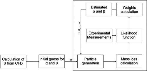
In Figure 1, the procedure adopted to estimate the mass transfer coefficient is summarized. The methodology consists of:

(2.1)	Adopting a corrosion model. For the present study, the double resistance model is adopted.
(2.2)	Obtaining the hydrodynamics pattern of the flow (experimentally or by CFD), more specifically obtaining the viscous sublayer thickness and the average effective diffusivity. This sublayer acts as a resistance, thus, the physical meaning i.e. the sublayer thickness, the fluid properties and the species transported in the fluid are carried in $\mathit{\beta }$ value.
(2.3)	Applying particle filters. The filter SIR and ASIR were chosen due to their particularity of being easily implemented, of filtering the uncertainties associated with measurements, and of their ability to estimate despite the scarce measurements. Both filters are initialized with values of $\mathit{\alpha }$ and $\mathit{\beta }$. The ‘guess’ value for $\mathit{\beta }$ comes from CFD, but $\mathit{\alpha }$ that also carries the physical meaning of the fluid and flow characteristics, as well as the thickness formed by the corrosion products (another resistance) does not have any traces that could be extracted from the experiment. For this reason, it is guessed with a magnitude order in accordance with the literature.

Figure 1. Methodology adopted to estimate the mass loss along the geometry.

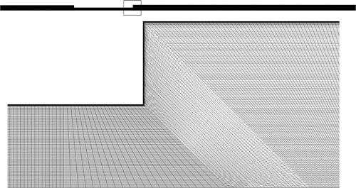
The experimental data of Lotz and Postlethwaite [38] were used to test the methodology developed here. The details of the experiment are described in [38]. Essentially, a saline solution is pumped through a nozzle with a contraction–expansion made of carbon steel. The contraction–expansion has an aspect ratio of 1.8:1:2. A schematic and the dimensions of the domain used for computational model purposes are shown in Figure 2. The authors performed 27 measurements along the geometry in two instant of time 25 and 48 h.

Figure 2. Computational domain utilized to simulate the experiment.

2.1. Corrosion model

It is accepted that corrosion of Fe happens by an anodic reaction and a cathodic reaction in acidic and neutral deaerated media [4,39,40]:(4) $$\begin{array}{c}\hfill 2Fe\to 2F{e}^{++}+4e^{-}\end{array}$$(4) (5) $$\begin{array}{c}\hfill 4H^{+}+4e^{-}⟶2H_2\end{array}$$(5)

In the presence of $O_2$, depolarization of the cathodic products takes place as(6) $$\begin{array}{c}\hfill O_2+2H_{2}O+4e^{-}⟶4O{H}^{-}\end{array}$$(6)

However, the reaction represented by Equation (6(6) $$\begin{array}{c}\hfill O_2+2H_{2}O+4e^{-}⟶4O{H}^{-}\end{array}$$(6) ) is in general so rapid that the kinetics of the reaction is controlled by the diffusion of oxygen to the reacting surface. Also, the rate of $O_2$, depolarization depends on the rate of the diffusion of $O_2$ through the resistant films at the surface of the metal. One of the diffusion resistances is due to the precipitation of corrosion product such as $Fe{\left(OH\right)}_2$ and $Fe{\left(OH\right)}_3$.(7) $$\begin{array}{cc}& Fe+H_{2}O+\frac{1}{4}{O}_2⟶Fe{\left(OH\right)}_2\hfill \end{array}$$(7) (8) $$\begin{array}{cc}& Fe{\left(OH\right)}_2+\frac{1}{2}{H}_{2}O+\frac{1}{4}{O}_2⟶Fe{\left(OH\right)}_3\hfill \end{array}$$(8)

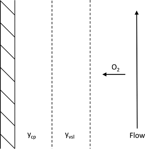
Mahato et al. [1,2] proposed a two series resistances diffusion model. In this case, dissolved $O_2$ in the flow must diffuse first through the fluid viscous sublayer and then through a porous corrosion zone to reach the material surface. Figure 3 presents a brief description of the model. In mathematical terms, the mass flux of $O_2$, n, is modelled as(9) $$\begin{array}{cc}\hfill \frac{\mathrm{d}n}{\mathrm{d}t}& =\frac{\left(D+D_t\right)\left(C_b-C_n\right)}{y_{vsl}}\hfill \end{array}$$(9) (10) $$\begin{array}{cc}\hfill \frac{\mathrm{d}n}{\mathrm{d}t}& =\frac{D\left(C_n-C_w\right)}{y_{cp}}\hfill \end{array}$$(10)

where D is the diffusivity of oxygen, $D_t$ is the eddy diffusivity coefficient, $C_b$ is the bulk concentration of $O_2$, $C_n$ is the concentration of $O_2$ at the interface between the solid wall and the turbulence boundary layer, $C_w$ is the concentration of $O_2$ at the surface of the base material, y is the length, the subscripts vsl refers to the viscous sublayer and cp to the corrosion products. The effective diffusivity is defined as the sum of the diffusivity and the eddy diffusivity, i.e. $D_{eff}=D+D_t$.

Figure 3. Sketch of the flow with mass transfer of oxygen to the surface causing the corrosion process.

By rewriting Equation (9(9) $$\begin{array}{cc}\hfill \frac{\mathrm{d}n}{\mathrm{d}t}& =\frac{\left(D+D_t\right)\left(C_b-C_n\right)}{y_{vsl}}\hfill \end{array}$$(9) ) and (10(10) $$\begin{array}{cc}\hfill \frac{\mathrm{d}n}{\mathrm{d}t}& =\frac{D\left(C_n-C_w\right)}{y_{cp}}\hfill \end{array}$$(10) ), in terms of mass transfer resistance, it becomes(11) $$\begin{array}{cc}\hfill \frac{\mathrm{d}n}{\mathrm{d}t}& =\frac{\left(C_b-C_n\right)}{R_{vsl}}\hfill \end{array}$$(11) (12) $$\begin{array}{cc}\hfill \frac{\mathrm{d}n}{\mathrm{d}t}& =\frac{\left(C_n-C_w\right)}{R_{cp}}\hfill \end{array}$$(12)

where R is the resistance, vsl is the viscous sublayer and cp is the corrosion products. The overall mass transfer resistance is(13) $$\begin{array}{c}\hfill R=R_{vsl}+R_{cp}\end{array}$$(13)

The resistance offered by the corrosion product layer is given by Equation (14(14) $$\begin{array}{c}\hfill y_{cp}={\int }_0^{t}r\frac{\mathrm{d}n}{\mathrm{d}t}\mathrm{d}t=rn\end{array}$$(14) ), assuming it to increase with the amount of corrosion and with a resistance coefficient r, which is independent of time t.(14) $$\begin{array}{c}\hfill y_{cp}={\int }_0^{t}r\frac{\mathrm{d}n}{\mathrm{d}t}\mathrm{d}t=rn\end{array}$$(14)

The retention factor F, proposed by Lotz and Postlethwaite [38], is defined in order to quantify the effects of erosion caused in the corrosion products thickness attached to the wall. It is written as(15) $$\begin{array}{c}\hfill F=\frac{\text{Local mass of scale}}{\text{Local metal mass loss}}\end{array}$$(15)

where $F=1.59$ for $FeO\left(OH\right)$ if all corrosion products are retained on the surface. As the reaction in the pipe wall surface is so rapid, the concentration of $O_2$ in the wall is considered zero or negligibly small in comparison to the concentration of $O_2$ in the flow. Thus, the mass flux of $O_2$ is then obtained:(16) $$\begin{array}{c}\hfill \frac{\mathrm{d}n}{\mathrm{d}t}=\frac{C_b}{\left(\frac{rn}{D}+\frac{y_{vsl}}{D_{eff}}\right)}\end{array}$$(16)

The amount of corrosion W in terms of $\mathit{\alpha }$ and $\mathit{\beta }$ is(17) $$\begin{array}{cc}\hfill \frac{\mathrm{d}W}{\mathrm{d}t}& =\frac{1}{2\mathit{\alpha }W+\mathit{\beta }}\hfill \end{array}$$(17) (18) $$\begin{array}{cc}\hfill \mathit{\alpha }& =\frac{r}{2D{C}_b}\hfill \end{array}$$(18) (19) $$\begin{array}{cc}\hfill \mathit{\beta }& =\frac{y_{vsl}}{D_{eff}{C}_b}\hfill \end{array}$$(19)  

2.2. CFD modelling

2.2.1. Conservation equations

The following conservation equations were used to simulate the fluid flow in the geometry detailed above. These equations are used to calculate the fields of pressure, velocity and concentration of species in the entire domain [41]. For a steady, incompressible flow and Newtonian fluid, the conservation of mass, momentum, species and turbulence are represented in Equations (20(20) $$\begin{array}{cc}\hfill \frac{\mathit{\partial }\left(\mathit{\rho }\overline{U_i}\right)}{\mathit{\partial }{x}_i}& =0\hfill \end{array}$$(20) )–(24(24) $$\begin{array}{cc}\hfill \frac{\mathit{\partial }\left(\mathit{\rho }\overline{U_i}\mathit{\omega }\right)}{\mathit{\partial }{x}_i}& ={\mathit{\alpha }}_{\mathit{\omega }}\mathit{\rho }{S}^2-{\mathit{\beta }}_{\mathit{\omega }}\mathit{\rho }{\mathit{\omega }}^2+\frac{\mathit{\partial }}{\mathit{\partial }{x}_i}\left[\left(\mathit{\mu }+{\mathit{\sigma }}_{\mathit{\omega }}{\mathit{\mu }}_t\right)\frac{\mathit{\partial }\mathit{\omega }}{\mathit{\partial }{x}_i}\right]\hfill \\ \hfill & +2\left(1-F_1^{\ast }\right)\mathit{\rho }{\mathit{\sigma }}_{w2}\frac{1}{\mathit{\omega }}\frac{\mathit{\partial }k}{\mathit{\partial }{x}_i}\frac{\mathit{\partial }\mathit{\omega }}{\mathit{\partial }{x}_i}\hfill \end{array}$$(24) ). Their respective boundary conditions are the same as used in [31](20) $$\begin{array}{cc}\hfill \frac{\mathit{\partial }\left(\mathit{\rho }\overline{U_i}\right)}{\mathit{\partial }{x}_i}& =0\hfill \end{array}$$(20) (21) $$\begin{array}{cc}\hfill \frac{\mathit{\partial }\left(\mathit{\rho }\overline{U_i{U}_j}\right)}{\mathit{\partial }{x}_j}& =\frac{\mathit{\partial }}{\mathit{\partial }{x}_j}\left[-p{\mathit{\delta }}_{ij}+\mathit{\mu }\left(\frac{\mathit{\partial }\overline{U_i}}{\mathit{\partial }{x}_j}+\frac{\mathit{\partial }\overline{U_j}}{\mathit{\partial }{x}_i}\right)-\mathit{\rho }\overline{u_i^{{}^{\prime }}{u}_j^{{}^{\prime }}}\right]+\mathit{\rho }{g}_i\hfill \end{array}$$(21) (22) $$\begin{array}{cc}\hfill \frac{\mathit{\partial }\left(\mathit{\rho }\overline{U_{j}C}\right)}{\mathit{\partial }{x}_j}& =\frac{\mathit{\partial }}{\mathit{\partial }{x}_j}\left[D\frac{\mathit{\partial }\left(\mathit{\rho }\overline{C}\right)}{\mathit{\partial }{x}_j}-\mathit{\rho }\overline{u_j^{{}^{\prime }}{c}^{{}^{\prime }}}\right]\hfill \end{array}$$(22)

where U is the velocity, C is the concentration of oxygen, p is the pressure, x is the axial coordinate, $\mathit{\rho }$ is the fluid density, $\mathit{\mu }$ is the dynamic viscosity, D is the diffusivity and g is the gravity. The turbulence models allow the calculation of the new terms introduced when the time-average equations for the momentum and species equation are solved. These terms are the Reynolds stresses, $-\mathit{\rho }\overline{u_i^{{}^{\prime }}{u}_j^{{}^{\prime }}}$, and the turbulent diffusion fluxes, $-\mathit{\rho }\overline{u_j^{{}^{\prime }}{c}^{{}^{\prime }}}$.

2.2.2. Turbulence model

The Shear Stress Transport (SST) k-$\mathit{\omega }$ proposed by Menter [42] is a model based on a blending function which ensures a proper selection of the k-$\mathit{ϵ}$ in free stream flow and k-$\mathit{\omega }$ in the near wall, where k is the turbulent kinetic energy, $\mathit{ϵ}$ is the turbulent dissipation and $\mathit{\omega }$ is the turbulent frequency. The equations’ formulations are given as:(23) $$\begin{array}{cc}\hfill \frac{\mathit{\partial }\left(\mathit{\rho }\overline{U_i}k\right)}{\mathit{\partial }{x}_i}& ={\tilde{P}}_k-{\mathit{\beta }}^{\ast }\mathit{\rho }k\mathit{\omega }+\frac{\mathit{\partial }}{\mathit{\partial }{x}_i}\left[\left(\mathit{\mu }+{\mathit{\sigma }}_k{\mathit{\mu }}_t\right)\frac{\mathit{\partial }k}{\mathit{\partial }{x}_i}\right]\hfill \end{array}$$(23) (24) $$\begin{array}{cc}\hfill \frac{\mathit{\partial }\left(\mathit{\rho }\overline{U_i}\mathit{\omega }\right)}{\mathit{\partial }{x}_i}& ={\mathit{\alpha }}_{\mathit{\omega }}\mathit{\rho }{S}^2-{\mathit{\beta }}_{\mathit{\omega }}\mathit{\rho }{\mathit{\omega }}^2+\frac{\mathit{\partial }}{\mathit{\partial }{x}_i}\left[\left(\mathit{\mu }+{\mathit{\sigma }}_{\mathit{\omega }}{\mathit{\mu }}_t\right)\frac{\mathit{\partial }\mathit{\omega }}{\mathit{\partial }{x}_i}\right]\hfill \\ \hfill & +2\left(1-F_1^{\ast }\right)\mathit{\rho }{\mathit{\sigma }}_{w2}\frac{1}{\mathit{\omega }}\frac{\mathit{\partial }k}{\mathit{\partial }{x}_i}\frac{\mathit{\partial }\mathit{\omega }}{\mathit{\partial }{x}_i}\hfill \end{array}$$(24)

where $F_1^{\ast }$ is the blending function, which is equal to zero in the region away from the surface ($k-\mathit{ϵ}$ turbulence model) and switches to one in the region inside the boundary layer (k-$\mathit{\omega }$ turbulence model). A limiter is used for the production term in order to prevent the build-up of turbulence in stagnation regions:(25) $$\begin{array}{c}\hfill \widetilde{P_k}=min(P_k,10·{\mathit{\beta }}^{\ast }\mathit{\rho }k\mathit{\omega }),P_k={\mathit{\mu }}_t{S}^2,S=\sqrt{2S_{ij}{S}_{ij}}\end{array}$$(25)

The eddy viscosity is defined as:(26) $$\begin{array}{c}\hfill {\mathit{\mu }}_t=\frac{\mathit{\rho }{a}^{\ast }k}{max(a^{\ast }\mathit{\omega },S{F}_2^{\ast })}\end{array}$$(26)

where $F_2$ is a second blending function.

Since the mechanism of turbulent transport of momentum and mass is the same, eddy mixing, it is expected that values of eddy diffusivity will be close to the turbulent viscosity. Thus, the turbulent Schmidt number is defined as:(27) $$\begin{array}{c}\hfill S{c}_t=\frac{{\mathit{\mu }}_t}{\mathit{\rho }{D}_t}\end{array}$$(27)

where the value considered for the turbulent Schmidt number is 0.9.

The constants are computed by linear combination of the corresponding constants of k-$\mathit{ϵ}$ and k-$\mathit{\omega }$ models through ${\mathrm{\Phi }}_3=F_1^{\ast }{\mathrm{\Phi }}_1+(1-F_1^{\ast }){\mathrm{\Phi }}_2$. The constants for this model are: ${\mathit{\beta }}^{\ast }=0.09$, ${\mathit{\alpha }}_{\mathit{\omega }1}=5/9$, ${\mathit{\beta }}_{\mathit{\omega }1}=3/40$, ${\mathit{\sigma }}_{k1}=0.85$, ${\mathit{\sigma }}_{\mathit{\omega }1}=0.5$, ${\mathit{\alpha }}_{\mathit{\omega }2}=0.44$, ${\mathit{\beta }}_{\mathit{\omega }2}=0.0828$, ${\mathit{\sigma }}_{k2}=1$, and ${\mathit{\sigma }}_{\mathit{\omega }2}=0.856$.

2.2.3. Turbulent boundary layer in a pipe flow

In a pipe flow, due to the proximity of the flow with the wall, the flow behaviour is essentially different from free turbulent flows [41]. In this case, the mean flow velocity near the wall only depends on the distance from the wall y, fluid density $\mathit{\rho }$, dynamic viscosity $\mathit{\mu }$ and wall shear stress ${\mathit{\tau }}_w$. Therefore, a dimensional analysis gives the law of the wall that contains the definition of the dimensionless velocity $u^{+}$ and dimensionless wall distance $y^{+}$:(28) $$\begin{array}{c}\hfill u^{+}=\frac{U}{u_{\mathit{\tau }}}=f\left(\frac{\mathit{\rho }{u}_{\mathit{\tau }}y}{\mathit{\mu }}\right)=f\left(y^{+}\right)\end{array}$$(28)

where the friction velocity is defined as(29) $$\begin{array}{c}\hfill u_{\mathit{\tau }}=\sqrt{\frac{{\mathit{\tau }}_w}{\mathit{\rho }}}\end{array}$$(29)

There are two regions that one can identify in the velocity profile. The first is the viscous sublayer that is in practice very thin ($y^{+}<5$) and the following relationship is valid:(30) $$\begin{array}{c}\hfill u^{+}=y^{+}\end{array}$$(30)

Outside the viscous sublayer ($30<y^{+}<500$) there is a region in which the viscous and inertial forces are both important. In this region, the log-law layer is(31) $$\begin{array}{c}\hfill u^{+}=\frac{1}{\mathit{\kappa }}ln\left(y^{+}\right)+B\end{array}$$(31)

where $\mathit{\kappa }$ is the von Kármán constant and B = 5.5 for smooth walls. In that manner, it is possible to obtain the viscous sublayer length by identifying both regions in the velocity profile.

Using a CFD software, the set of differential equation is solved. Two distinct models for the wall treatment were used. The wall function model uses empirical formulas that impose appropriate conditions near the wall, without fully resolving the boundary layer, thus saving computational resources. The Low Reynolds Number (LRN) turbulence model solves the details of the viscous sublayer and the diffusion-controlled concentration boundary layer, improving the accuracy near the wall. In the case of turbulence models based on the k-$\mathit{ϵ}$ model, the wall function method is implemented, so the resolution of the boundary layer is limited. The turbulence models based on the $\mathit{\omega }$ equation, such as SST k-$\mathit{\omega }$, are more suitable for implementing the LRN turbulence model.

2.3. The sampling importance resampling and auxiliary sampling importance resampling

Particle filters provide an attractive framework for issues in estimates of poorly known parameters as well as improving predictions [43]. This section gathers the most important information to be implemented from SIS algorithm, the base algorithm to SIR and ASIR. Since the present paper does not offer any new developments to the algorithm, but rather, supplies a new use for it, the information in reference the minutiae of particle filters requirements, and definitions of mathematical quantities are not developed here, but can be found in [44–48].

Most particle filters rely on the Sequential Importance Sampling (SIS). This algorithm is based on the calculation of an importance density, i.e. a density that is used to build the particles instead of the exact posterior density that cannot be exactly computed. The PDF of the control vector x is sampled with N particles. We consider the set of particles $\left\{{\widehat{x}}_{0:k}^i,i=1,\dots ,N\right\}$ associated with the normalized weights $\left\{w_k^i,i=1,\dots ,N\right\}$, satisfying

${\sum }_{i=1}^N{w}_k^i=1.$ Let the particles be drawn from a proposal distribution called importance density in a way that ${\widehat{x}}^i\sim q(\widehat{x})$, i = 1, ..., N and let $\mathit{\pi }(\widehat{x})$ be the probability density. The posterior density at time instant $t_k$ can be discretely approximated by [45,49–54]:(32) $$\begin{array}{c}\hfill \mathit{\pi }({\widehat{x}}_k|z_{1:k}^{obs})\approx \sum _{i=1}^N{w}_k^i\mathit{\delta }\left({\widehat{x}}_k-{\widehat{x}}_k^i\right)\end{array}$$(32)

with $\mathit{\delta }\left(.\right)$ being the Dirac delta function ant the weights computed from [50]:(33) $$\begin{array}{c}\hfill w_k^i\propto w_{k-1}^i\frac{\mathit{\pi }\left(z_k^{obs}|{\widehat{x}}_k^i\right)\mathit{\pi }\left({\widehat{x}}_k^i|{\widehat{x}}_{k-1}^i\right)}{q\left({\widehat{x}}_k^i|{\widehat{x}}_{k-1}^i,z_k^{obs}\right)}\end{array}$$(33)

where the importance density $q({\widehat{x}}_k^i|{\widehat{x}}_{k-1}^i,z_k^{obs})$ is assumed to be a Markovian process. There are two ways to choose the importance density. The optimal choice, which minimizes the variance of the importance weights conditioned upon control parameters ${\widehat{x}}_{k-1}^i$ and measurements $z_k^{obs}$ , is given by $q({\widehat{x}}_k^i|{\widehat{x}}_{k-1}^i,z_k^{obs})=\mathit{\pi }\left({\widehat{x}}_k^i|{\widehat{x}}_{k-1}^i,z_k^{obs}\right)$. The Equation (33(33) $$\begin{array}{c}\hfill w_k^i\propto w_{k-1}^i\frac{\mathit{\pi }\left(z_k^{obs}|{\widehat{x}}_k^i\right)\mathit{\pi }\left({\widehat{x}}_k^i|{\widehat{x}}_{k-1}^i\right)}{q\left({\widehat{x}}_k^i|{\widehat{x}}_{k-1}^i,z_k^{obs}\right)}\end{array}$$(33) ) becomes(34) $$\begin{array}{c}\hfill w_k^i\propto w_{k-1}^i\mathit{\pi }\left(z_k^{obs}|{\widehat{x}}_{k-1}^i\right)\end{array}$$(34)

However, for most practical problems, this optimal choice is not analytically tractable and a suboptimal importance density is taken as the transition prior, that is, $q({\widehat{x}}_k^i|{\widehat{x}}_{k-1}^i,z_k^{obs})=\mathit{\pi }({\widehat{x}}_k^i|{\widehat{x}}_{k-1}^i)$ [50], so that Equation (33(33) $$\begin{array}{c}\hfill w_k^i\propto w_{k-1}^i\frac{\mathit{\pi }\left(z_k^{obs}|{\widehat{x}}_k^i\right)\mathit{\pi }\left({\widehat{x}}_k^i|{\widehat{x}}_{k-1}^i\right)}{q\left({\widehat{x}}_k^i|{\widehat{x}}_{k-1}^i,z_k^{obs}\right)}\end{array}$$(33) ) reduces to(35) $$\begin{array}{c}\hfill w_k^i\propto w_{k-1}^i\mathit{\pi }\left(z_k^{obs}|{\widehat{x}}_k^i\right).\end{array}$$(35)  

2.3.1. SIR filter

The application of the SIS particle filter might result in the degeneracy problem, meaning that after a couple of estimations all but very few particles will have negligible weights [45,49–54]. If this problem occurs, a large computational effort is devoted to updating particles whose contribution to the approximation of the posterior is almost zero. In practice, this problem can be overcome by adding a resampling step in the SIS particle filter algorithm. The resampling process involves a mapping of the random measures $\left\{{\widehat{x}}_k^i,w_k^i\right\}$ into $\left\{{\widehat{x}}_k^{i\ast },1/N\right\}$ with uniform weights equal to 1 / N with N the number of particles. This leads to the elimination of particles with low weights and additional sampling in the vicinity of the particles with high weights effective particles. Resampling could be performed if the number of effective particles falls below a certain threshold number, but in the following we choose to apply the resampling process indistinctively at every time $t_k$. Such algorithm is called Sampling Importance Resampling (SIR) filter [50].

2.3.2. ASIR filter

Although the resampling step reduces the effects of the degeneracy problem, it may lead to a loss of diversity and the resultant sample may contain many repeated particles. Hence, despite the fact that in the SIR algorithm the weights are easily computed and the importance density can be easily sampled, the particles may experience a fast loss of diversity. Indeed, this problem, known as sample impoverishment, can be severe in the case of small state evolution noise [45,49,50,54]. In addition, in the SIR algorithm the state space is explored without the information conveyed by the measurements, that is, the particles at each time instant are generated through the sole application of the transition prior $\mathit{\pi }({\widehat{x}}_k^i|{\widehat{x}}_{k-1}^i)$. With the ASIR algorithm an attempt is made to overcome these drawbacks, by performing the resampling step at time $t_{k-1}$, with the available measurement at time $t_k$ [50]. The resampling is based on some point estimate ${\mathit{\xi }}_k^i$ that characterizes $\mathit{\pi }({\widehat{x}}_k|{\widehat{x}}_{k-1}^i)$, which can be the mean of $\mathit{\pi }({\widehat{x}}_k|{\widehat{x}}_{k-1}^i)$ or simply a sample of $\mathit{\pi }({\widehat{x}}_k|{\widehat{x}}_{k-1}^i)$. If the state evolution model noise is small, $\mathit{\pi }({\widehat{x}}_k|{\widehat{x}}_{k-1}^i)$ is generally well characterized by ${\mathit{\xi }}_k^i$, so that the weights $w_k^i$ are more even and the ASIR algorithm is less sensitive to outliers than the SIR algorithm. On the other hand, if the state evolution model noise is large, the single point estimate ${\mathit{\xi }}_k^i$ in the state space may not characterize well $\mathit{\pi }({\widehat{x}}_k|{\widehat{x}}_{k-1}^i)$ and the ASIR algorithm may not be as effective as the SIR algorithm.

3. Results and discussion

3.1. Concerns from the CFD modelling

The schematic and the dimensions of the domain used for computational model purposes were already shown in Figure 2. The Reynolds number was $3.4\times {10}^5$ in the minor section and $1.7\times {10}^5$ in the large sections. It was assumed to have a steady state and turbulent flow, with a Schmidt Number of 369, and the salt water saturated with oxygen has a concentration of 6.23 mg$·$L^-1 [31,55]. As the experimental set-up was isothermal, the equation of energy was not solved and since no information about the pH was provided, it was considered the same as the salt water for all experiments.

3.1.1. Mesh verification

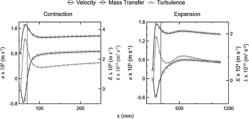
The mesh was made with a high density of nodes near the wall, so it could reach an appropriate $y^{+}$ value and fully resolve the boundary layer, Figure 4. To investigate whether the mesh interferes with the results, the influence of the grid is analysed. The conducted simulations tested four different mesh node densities in the near-wall region. The information about the meshes can be seen in Table 1. The results presented in Figure 5 show convergence tests for velocity, the turbulence kinetic energy and the mass transfer coefficient along the boundary layer at two different zones in geometry: the first starting slightly downstream of the contraction; the second slightly downstream of the expansion. The discrepancies of the mass transfer coefficient in Mesh 1 indicate that the diffusive boundary layer is not properly solved. For Mesh 2, the calculation was not enough satisfactory showing some fluctuations on velocity and turbulence energy profiles. Unlike what was observed, the results for the Mesh 3 and 4 showed that the boundary layer is already correctly solved, in this way Mesh 4 was used for the calculations.

Figure 4. Mesh grid utilized to solve the transport equations.

Figure 5. Near-wall velocity, mass transfer and turbulence along the contraction and the expansion for different meshes.

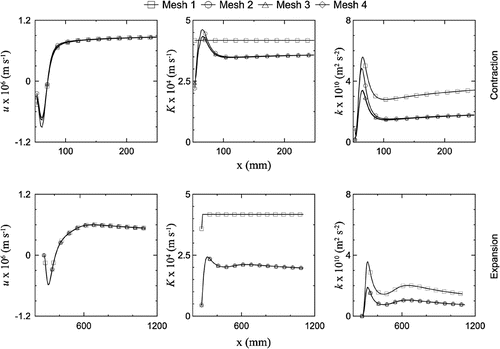
Table 1. Number of nodes and elements of the meshes.

Mesh	Number of nodes	Number of elements
1	869,440	431,844
2	1,295,420	644,112
3	1,418,000	705,256
4	2,127,000	1,059,656

3.1.2. The hydrodynamics on mass transfer coefficient

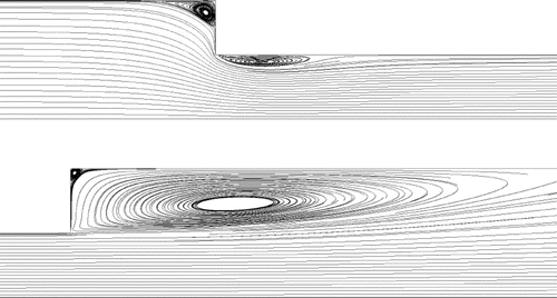
The streamlines for this typical case can be viewed in Figure 6. The region of recirculating flow is developed as a consequence of the sudden change in the geometry section (the contraction and the expansion). In these regions, the boundary layer detaches creating backward flows (as reported in the literature [21]) directly related to the increase of mass transfer coefficient and turbulence kinetic energy as viewed in Figure 7. One can see the typical velocity distribution over x-direction inside the viscous boundary layer. The negative velocities, highlighted in Figure 7, indicate the zone where the boundary layer is detached from the core flow, and where the mass transfer coefficient suddenly increases accompanied by a strong fluctuation on turbulence energy.

Figure 6. Recirculations in the contraction and expansion respectively.

Figure 7. Near-wall velocity compared with turbulence and mass transfer along the contraction and expansion region.

3.1.3. A first estimate of $\mathit{\beta }$ value

The effective diffusivity and velocity are shown along the boundary layer at five points in the x-direction. Three upstream of the contraction (at 6.8 mm, 26.5 mm, 43.5 mm), one in the contraction (at 55.5 mm) and one downstream of the expansion (at 318.3 mm). The location of these points were chosen to illustrate the methodology proposed in the present work, but they were analysed in all experimental position measured by Lotz and Postlethwaite [38]. In Figure 8, at each chosen point, the velocity and effective diffusivity profile was plotted to infer the viscous sublayer thickness and to calculate the average of the effective diffusivity. The viscous sublayer was obtained by identifying the regions explained in Section 2.2.3 and the turbulent diffusivity was obtained by Equation (27(27) $$\begin{array}{c}\hfill S{c}_t=\frac{{\mathit{\mu }}_t}{\mathit{\rho }{D}_t}\end{array}$$(27) ). Thus, in the upstream points the viscous sublayer thickness through which oxygen diffuses is about 2 mm and its respective average diffusivities are approximately $4.19\times {10}^{-5}$, $4.09\times {10}^{-5}$, $1.54\times {10}^{-5}{\text{m}}^2{\text{s}}^{-1}$. In the contraction (at 55.5 mm) , the thickness is 1 mm and the diffusivity is $1.34\times {10}^{-5}{\text{m}}^2{\text{s}}^{-1}$. After expansion, at 318.3 mm, the thickness is 4 mm with $4.74\times {10}^{-5}{\text{m}}^2{\text{s}}^{-1}$ of average diffusivity. These values are then used to calculate $\mathit{\beta }$ from Equation (19(19) $$\begin{array}{cc}\hfill \mathit{\beta }& =\frac{y_{vsl}}{D_{eff}{C}_b}\hfill \end{array}$$(19) ).

3.2. Applying particle filters

The adopted corrosion model, Equation (17(17) $$\begin{array}{cc}\hfill \frac{\mathrm{d}W}{\mathrm{d}t}& =\frac{1}{2\mathit{\alpha }W+\mathit{\beta }}\hfill \end{array}$$(17) ), is now applied to predict mass losses of the base material. The experimental data were recovered from Lotz and Postlethwaite [38], which describes in detail providing sufficient information about the geometry dimension, fluid properties, fluid dynamics and mass loss data given in two instants, 25 h and 48 h. The mass losses were measured along 27 spatial positions, some of them were already shown in Figure 8. The measurements were performed in a roughened surface at 25 h and in a smooth surface at 48 h. Due to the unknown nature of the resistance coefficient presented in the model, two inverse problem techniques are implemented in FORTRAN language. In that manner, particle filters SIR and ASIR algorithms are applied in the corrosion problem to estimate the mass loss caused by mass transfer of oxygen to the reacting surface. Each position was evaluated separately, in a way that the problem was treated as a function of the time only. At the target point, both SIR and ASIR filters were employed. Particles of alpha and beta were generated from the prior information and then, after evaluating the mass loss, compared with measurements. Thereby, an estimated value of alpha and beta in each time was obtained for this position. This methodology was repeated for all positions. After that, each estimated variable is now used to calculate the mass loss rate by Equation (17(17) $$\begin{array}{cc}\hfill \frac{\mathrm{d}W}{\mathrm{d}t}& =\frac{1}{2\mathit{\alpha }W+\mathit{\beta }}\hfill \end{array}$$(17) ). The retention factor is calculated by Equation (15(15) $$\begin{array}{c}\hfill F=\frac{\text{Local mass of scale}}{\text{Local metal mass loss}}\end{array}$$(15) ) and compared with the data from [38] after evaluating the mass loss rate and mass scale using information of the state variables.

3.2.1. Sensibility analysis

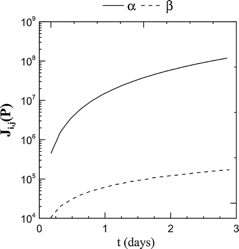
In order to examine if the parameters could be estimated, a sensitivity analysis should always be performed. The sensitivity coefficient plays an important role in state estimation problems [56]. It is defined as(36) $$\begin{array}{c}\hfill J_{ij}\left(P\right)=\frac{\mathit{\partial }{W}_i}{\mathit{\partial }{P}_j}\end{array}$$(36)

where i is the total number of measurements and j is the total number of unknown state variables.

A relatively small value of the magnitude of $J_{ij}$ indicates that large changes in $P_j$ yield small changes in $W_i$ and it becomes a very difficult task to estimate the state variable because basically the same value for mass loss would be obtained for a wide range of values of $P_j$. The results can be seen in Figure 9. It is evident analysing the sensitivity of the variables that beta is difficult to estimate due to the lower sensitivity compared to alpha. In other words, the inverse problem is not very sensitive to beta values, when compared to alpha. Physically, it means that a finer measurement of beta via experiment or CFD is necessary.

3.2.2. The solution of the direct and inverse problems

The direct problem was solved using the Runge–Kutta method. Measurements performed by [38] over the length of a 1.8:1:2 contraction–expansion in the two distinct instants were used again for comparison and estimation of the state variables. An error of 1 % of the maximum value of the measures were used in the measurement errors matrix. The chosen state variables were alpha and beta. The evolution model defined for them is a random walk as given(37) $$\begin{array}{c}\hfill W_k=W_{k-1}+\mathit{\sigma }{X}^i\end{array}$$(37)

where $X^i$ are random numbers with normal distribution, zero mean and unitary standard deviation. The standard deviations are 0.5, 0.3 to model evolution in time for alpha and beta, respectively.

Two different initial guess set-ups were chosen. The first one (IG1), in the same order of magnitude as [1,2], has a value of $3\times {10}^6\text{day}{\text{dm}}^4{\text{mg}}^{-2}$ for alpha and a value of $3\times {10}^4\text{day}{\text{dm}}^2{\text{kg}}^{-1}$ for beta. In the second set-up (IG2), beta was calculated via CFD, due to the fact that beta parameters depend only on the flow, according to Equation (19(19) $$\begin{array}{cc}\hfill \mathit{\beta }& =\frac{y_{vsl}}{D_{eff}{C}_b}\hfill \end{array}$$(19) ). Table 2 indicates the initial guesses in all positions along the geometry.

The number of particles used to advance alpha and beta in time were 100, 1000 and 10,000 for the SIR and the ASIR filters. In Figure 10, it is possible to see that IG2 obtained an estimation with a better convergence than IG1, when the number of particles influence is analysed, for both the SIR and the ASIR filters while IG1 data were scattered around the experimental data. This behaviour could be an indication of a greater predictive likelihood of IG2, being indeed suitable to use CFD to improve the prior information of the state variable. The same trends were noted in all other positions. The average time elapsed to estimate the quantities are shown in Table 3. It can be noticed that the estimations increase by an amount that is not significantly higher when comparing 1000 with 10,000. For this reason, all results were analysed with 10,000 particles.

Figure 8. Effective diffusivity and velocity boundary layer in the recirculation zone, upstream of the reattachment point.

Figure 9. Sensitivity analysis for the parameters alpha and beta over time.

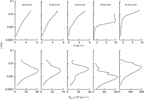
Figure 10. Corrosion rate over time at 318.3 mm, for different numbers of particles and estimated with IG1 and IG2 by the SIR and ASIR filters.

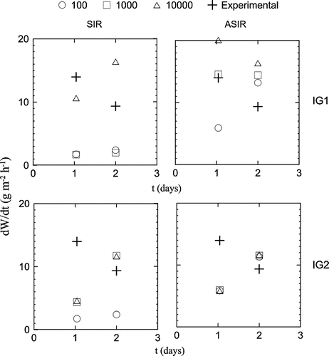
Figure 11. Estimated mass loss through the geometry with the SIR filter and the ASIR filter in 25 and 48 h with IG1 and IG2.

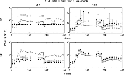
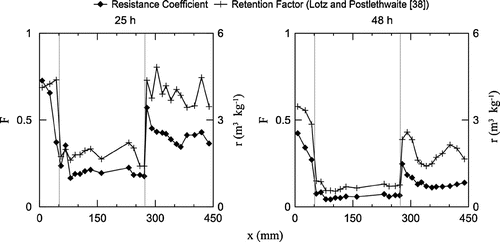
Figure 12. Estimated retention factor through the geometry with the SIR filter and the ASIR filter in 25 and 48 h with IG2.

Figure 13. Resistance coefficient and retention factor along the x-direction in 25 and 48 h.

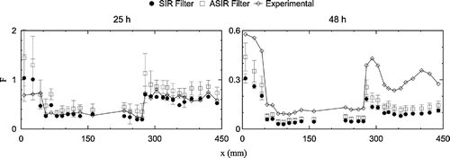
Figure 14. Synthesis of the results obtained by estimating the state variables utilizing the corrosion model. (a) Change over time of the state variables alpha and beta. (b) Dimensionless number analysis in the geometry. (c) Corrosion scale thickness along the x-direction. (d) Corrosion rates in the base material.

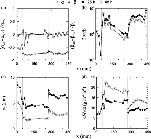
Table 2. Initial guess assisted by the CFD.

	Upstream of the expansion			Downstream of the expansion
x	$\mathit{\alpha }\times {10}^6$	$\mathit{\beta }\times {10}^6$	x	$\mathit{\alpha }\times {10}^6$	$\mathit{\beta }\times {10}^6$
(mm)	$(\text{day}{\text{dm}}^{-4}{\text{mg}}^{-2})$	$(\text{day}{\text{dm}}^{-2}{\text{mg}}^{-1})$	(mm)	$(\text{day}{\text{dm}}^{-4}{\text{mg}}^{-2})$	$(\text{day}{\text{dm}}^{-2}{\text{mg}}^{-1})$
6.8		11.73	278.2		10.67
26.5		13.51	291.0		3.54
43.5		47.37	303.8		2.13
55.5		3.61	318.3		1.66
67.4		1.41	327.6		1.91
80.2		1.57	340.4	3.00	1.86
92.2		2.01	354.9		1.84
104.9	3.00	2.33	366.0		1.72
117.7		2.61	382.3		1.75
132.3		2.99	401.9		1.79
160.4		3.88	419.8		1.78
231.2		6.02	439.4		0.98
244.0		6.52
260.2		7.01
271.3		7.21

Table 3. Average time elapsed estimating the values in each position along the geometry.

Particle	SIR filter (s)	ASIR filter (s)
100	0.03 $\pm$ 0.01	0.16 $\pm$ 0.01
1000	52 $\pm$ 5	36 $\pm$ 2
10,000	172 $\pm$ 9	235 $\pm$ 45

Table 4. Alpha and beta estimated with IG1.

	SIR filter				ASIR filter
	$\mathit{\alpha }\times {10}^8$		$\mathit{\beta }\times {10}^4$		$\mathit{\alpha }\times {10}^8$		$\mathit{\beta }\times {10}^4$
	$(\text{day}{\text{dm}}^{-4}{\text{mg}}^{-2})$		$(\text{day}{\text{dm}}^{-2}{\text{mg}}^{-1})$		$(\text{day}{\text{dm}}^{-4}{\text{mg}}^{-2})$		$(\text{day}{\text{dm}}^{-2}{\text{mg}}^{-1})$
x (mm)	25 h	48 h	25 h	48 h	25 h	48 h	25 h	48 h
6.8	4.64	6.81	3.08	5.00	7.41	10.27	2.53	3.16
26.5	4.64	6.71	3.08	4.19	2.28	3.16	4.01	5.61
43.5	4.64	5.48	3.08	3.74	7.65	7.20	2.47	2.39
55.5	4.64	1.28	3.08	0.85	0.82	0.89	2.07	2.19
67.4	4.64	1.67	3.08	0.89	3.27	1.70	1.58	1.59
80.2	4.64	1.02	3.08	0.09	1.09	0.78	1.23	1.35
92.2	4.64	0.80	3.08	0.55	0.80	0.64	1.85	1.32
104.9	4.64	1.09	3.08	0.61	0.81	0.73	1.80	1.60
117.7	4.64	0.20	3.08	1.14	0.80	0.70	1.84	1.64
132.3	4.64	1.67	3.08	0.12	0.82	0.88	2.00	1.69
160.4	4.64	0.09	3.08	1.61	0.81	0.76	1.92	1.78
231.2	4.64	0.77	3.08	1.29	3.25	1.37	1.50	1.41
244.0	4.64	1.72	3.08	0.01	0.82	0.82	2.06	1.87
260.2	4.64	1.50	3.08	0.58	0.81	0.90	1.96	1.90
271.3	4.64	0.98	3.08	0.86	0.81	0.79	1.96	1.96
278.2	4.64	4.69	3.08	3.11	6.65	5.49	2.50	2.63
291.0	4.64	2.64	3.08	2.02	0.68	1.23	2.95	4.74
303.8	4.64	2.59	3.08	1.62	0.67	1.04	2.78	4.55
318.3	4.64	2.25	3.08	1.30	0.67	0.67	2.78	3.79
327.6	4.64	1.80	3.08	1.80	0.67	0.95	2.72	3.96
340.4	4.64	1.35	3.08	1.68	2.33	2.34	2.01	1.95
354.9	4.64	1.79	3.08	1.08	3.23	2.53	1.55	1.57
366.0	4.64	1.80	3.08	1.07	3.09	3.65	1.45	0.75
382.3	4.64	1.72	3.08	1.40	0.67	0.73	2.76	3.39
401.9	4.64	1.90	3.08	1.26	0.68	0.91	2.76	3.36
419.8	4.64	1.66	3.08	1.76	0.68	0.51	2.87	3.94
439.4	4.64	1.76	3.08	1.38	3.10	2.95	1.48	2.07

Table 5. Alpha and beta estimated with IG2.

	SIR filter				ASIR filter
	$\mathit{\alpha }\times {10}^8$		$\mathit{\beta }\times {10}^6$		$\mathit{\alpha }\times {10}^8$		$\mathit{\beta }\times {10}^6$
	$(\text{day}{\text{dm}}^{-4}{\text{mg}}^{-2})$		$(\text{day}{\text{dm}}^{-2}{\text{mg}}^{-1})$		$(\text{day}{\text{dm}}^{-4}{\text{mg}}^{-2})$		$(\text{day}{\text{dm}}^{-2}{\text{mg}}^{-1})$
x (mm)	25 h	48 h	25 h	48 h	25 h	48 h	25 h	48 h
6.8	5.08	1.56	7.93	8.54	3.33	1.59	9.27	8.62
26.5	4.95	1.32	9.26	7.79	3.01	1.28	12.90	12.90
43.5	2.35	1.04	23.19	22.59	1.70	1.02	51.80	52.91
55.5	1.28	0.30	3.88	4.57	1.08	0.28	3.06	3.59
67.4	2.37	0.31	1.70	2.17	1.62	0.31	1.47	0.79
80.2	1.28	0.15	1.72	1.75	0.76	0.16	1.65	1.78
92.2	1.28	0.15	2.15	2.55	0.87	0.16	1.53	1.00
104.9	1.47	0.18	1.35	1.12	0.87	0.20	1.72	1.69
117.7	1.47	0.20	1.54	1.28	0.94	0.19	1.24	1.25
132.3	1.28	0.23	3.23	3.64	0.98	0.22	2.77	2.91
160.4	1.48	0.22	2.18	2.48	0.89	0.22	2.92	2.90
231.2	1.28	0.26	6.46	4.59	1.03	0.27	5.81	5.76
244.0	1.18	0.23	5.56	6.43	0.84	0.22	5.72	6.69
260.2	0.95	0.24	7.63	8.69	0.84	0.25	5.30	5.57
271.3	0.95	0.24	7.85	8.22	0.81	0.25	5.49	4.61
278.2	3.45	0.93	10.66	9.51	2.62	0.93	11.13	11.56
291.0	3.26	0.68	3.67	3.40	2.07	0.69	3.82	3.79
303.8	3.19	0.65	1.59	1.48	1.98	0.63	2.43	2.40
318.3	3.12	0.49	1.58	1.13	1.96	0.49	1.86	1.65
327.6	3.05	0.52	1.84	1.57	1.93	0.53	1.72	1.56
340.4	2.88	0.45	1.84	1.31	1.78	0.45	1.87	1.95
354.9	2.37	0.40	2.19	1.77	1.65	0.42	1.76	1.65
366.0	2.68	0.45	0.89	0.69	1.58	0.43	1.59	1.72
382.3	3.01	0.47	1.67	1.20	1.89	0.44	1.57	1.53
401.9	3.01	0.47	1.77	1.26	1.90	0.45	1.81	1.96
419.8	3.20	0.50	1.44	1.02	1.97	0.49	2.40	2.30
439.4	2.56	0.57	1.02	0.99	1.67	0.52	1.00	1.08

Once defined the minimum required number of particles, the influence of the initial guesses on the estimated alpha and beta was investigated, in Figure 11. It is clear that the SIR filter at the time where measurements were carried out presented poor particle diversity, thus the filter were not able to estimate the variables with accuracy. This computational issue is more pronounced at 25 h in the contraction zone, where the standard deviation of the particles was null, implying that all particles have the same value. When the initial guess is improved via CFD calculation, it overcomes the loss of sampling diversity problem exposing the SIR dependence on the prior information quality. Overall, the estimates of the ASIR filter had a better accuracy than the SIR filter. Figure 12 compares the retention factor, which is directly related to the corrosion products, estimated with IG2 as prior information. The retention factor obtained by IG1 greatly underestimates the quantity due to the fact that beta is higher for IG1, in that manner it is not shown. It can be observed that both the estimations performed by SIR and ASIR filter presented a good agreement with the experimental data.

The disparities between experimental data and the predictions were due to two primary reasons. Firstly, it is noticeable that the filters underperformed the estimations for 25 h for the mass loss rates, Figure 11, while the errors between experimental data and estimated values of the corrosion products were considerably smaller, Figure 12. This behaviour can be explained by the fact that all mass losses measured by [38] in 25 h were conducted on a roughened surface, while the measurements in 48 h were conducted in a smooth surface. When the phenomenon happens on roughened surfaces, it is reported to produce an enhancement of around 100% [38] in oxygen mass transfer, explaining the offset presented in 25 h. A correction factor between 1 and 2 is recommended by [38] to account for the roughness influence. Secondly, there are uncertainties in measurements utilized to estimate the state variables. The data lack information on the amount of mass loss evolution in time that was required in the inverse problem technique, informing only the mass loss rate in 25 and 48 h. The mass loss rate was considered constant along the considered time to evaluate the amount of mass loss experimentally, thus applying considerable uncertainties. In that manner, the observations used to estimate the state variables are overestimated, which is more pronounced at 48 h as the error is cumulative in time.

Another source of uncertainties is the dependence with time of the resistance coefficient, Equation (14(14) $$\begin{array}{c}\hfill y_{cp}={\int }_0^{t}r\frac{\mathrm{d}n}{\mathrm{d}t}\mathrm{d}t=rn\end{array}$$(14) ). To develop the model, it is assumed that the resistance coefficient is time independent, which is clearly a wrong assumption. Figure 13 shows the estimated resistance coefficient compared with the retention factor, at 25 and 48 h. The application of the particle filters shows that the resistance coefficient is indeed dependent on the time, so the assumption adopted in this model imposes a considerable error in the analysis. Despite all these uncertainties and errors, the particle filter estimated the variables in this application fairly well and presented a satisfactory agreement with the experimental data. It can also be observed that the resistance coefficient could be related to the retention factor. This physical quantity indicates the erosion occurring in the base material. The resistance coefficient, in that manner, may provide information about the erosion of the base material and the morphology of the corrosion products as well, although further investigation is required to confirm suspicions.

Detailed information about the quantities estimated, alpha and beta, are provided in Tables 4 and 5. Some aspects are relevant in this matter. It is evident that no significant change of beta over time occurred when estimating by the particle filter, indicating that the flow does not depend on time, i.e. the flow is steady and beta values estimated using IG1 deviated little from the value firstly set, which reinforces the idea of the difficulty of estimating the quantity. The use of CFD in this way provided a better prediction of the corrosion along the geometry, as it is shown on Figure 11. Also, the estimated values of beta is reduced on average by two orders of magnitude when compared IG2 with IG1, which is in agreement with the phenomena. The reduction in beta may be explained by the thickening of the viscous sublayer that would occur in the flow due to the increase of the inertial forces. Experiments performed by Mahato [1,2] has a maximum Reynolds number of $4.5\times {10}^4$ while the experiments performed by Lotz and Postlethwaite [38] are between $1.7\times {10}^5$ and $3.4\times {10}^5$.

Analysing the results obtained by the particle filters applied in the current work gives insights of the phenomena. Figure 14 summarizes the main points that the particle filters could estimate. Figure 14(a) shows the variations along the time of alpha and beta quantities, Figure 14(b) the dimensionless number related to the resistances is shown along the x-direction over time, Figure 14(c) provides information about the evolution in time of the corrosion products retained in the inner wall and Figure 14(d) shows the increase of mass loss rate over time. It can be noticed that, on average, beta remains constant, indicating that the flow is indeed steady on average, while there is a considerable variation of alpha, shown in Figure 14(a). Thus, the reduction in alpha directly implies on the resistance to corrosion, which is lower in 48 h, as one can see in Figure 14(b). The dimensionless number indicates that, although a considerable reduction of alpha occurred, the influence of the corrosion products changed only slightly. The main resistance to corrosion still remains the corrosion products, with the viscous sublayer having little influencing. This reduction is caused by the removal of the corrosion scale, Figure 14(c), by erosion, which is flow induced, that protects the base material from corrosion. The removal of this protection directly impacts the corrosion rates, Figure 14(d), that increases considerably in time.

4. Conclusion

In the present work, a methodology was proposed to deal with the flow-accelerated corrosion problem. Particle filters were used as a statistical approach to estimate corrosion rate and CFD technique utilized to improve the information about the state variable beta, which is flow dependent only, providing a better initial guess to be applied in the particle filters. Two different particle filters were then successfully implemented, the SIR and ASIR filters.

Concerning the physical representativeness of the model, as the model used does not carry physical information about the roughness of the wall and one assumes that the integral given by Equation (14(14) $$\begin{array}{c}\hfill y_{cp}={\int }_0^{t}r\frac{\mathrm{d}n}{\mathrm{d}t}\mathrm{d}t=rn\end{array}$$(14) ) is constant with time, the filter underestimates the corrosion rate for 25 h, nevertheless, for this same instant the filters have a realistic estimation of the retention factor. For 48, the filter overestimate corrosion rate and underestimate the retention factor. It is important to emphasize that a relationship may exist between the resistance coefficient and the retention of the products in the base material wall, implying that the resistance coefficient carries the information about the erosion of the corrosion products by the flow. It could be inferred by plotting the resistance coefficient and retention factor along the x-direction in 25 and 48 h, where, estimations of the particles filter represented in this case by the resistance coefficient follow the same trend of the retention factor calculated in [38].

The CFD results were in agreement with flow pattern in the reported literature, therefore, the beta value obtained from these results and from the literature were implicitly compared by means of the estimated corrosion rate. The improvement on the Initial Guess quality showed a significant reduction in the relative error when ASIR filter was applied, in 3.5 % for 25 h and in 39 % for 48 h.

The methodology could evaluate the erosion caused by the flow, showing that in 48 h, the corrosion scale diminished, thus increasing the corrosion rates as the resistance to the oxygen diffusion became lower. Also, the advantage of the presented methodology is a local and transient estimation of the corrosion rate following closely the trend of the experiments that is clearly a stochastic phenomenon, but commonly reduced as a flow induced problem.

Finally, the case utilized to implement this procedure was FAC in an aqueous aerated with 3% NaCl solution. The methodology should work for another type of corrosion, although it must be important to highlight the dependency of the current forward problem to the kinetics of the reactions considered for this medium. The double resistance layer is indicated to the mechanism of oxygen transport and scale formation on a ferrous surface. For other types of mechanism, a different forward problem must be considered.

5. Nomenclature

5.1. Latin letters

• a Constant potency relating Reynolds number and Sherwood number

• $a^{\ast }$ Constant of the SST model

• B Constant of the log-law model

• b Constant potency relating Schmidt number and Sherwood number

• C Concentration, $\text{kg}{\text{m}}^{-3}$

• $\overline{C}$ Mean concentration, $\text{kg}{\text{m}}^{-3}$

• c Constants related to the corrosion model fitted with least squares

• $c^{\prime }$ Concentration fluctuation, $\text{kg}{\text{m}}^{-3}$

• D Oxygen diffusivity in water solution, ${\text{ms}}^{-1}$

• d Tube diameter, m

• F Retention factor

• $F^{\ast }$ Blending function

• g Gravity, ${\text{ms}}^{-2}$

• J Sensibility coefficient

• K Mass transfer coefficient, ${\text{ms}}^{-1}$

• k Turbulent kinetic energy, ${\text{m}}^2{s}^{-2}$

• n Amount of mass, $\text{kg}{\text{m}}^{-2}$

• $\dot{n}$ Mass flux, $\text{kg}{\text{m}}^{-2}{s}^{-1}$

• P Parameter

• $P_k$ Production term, $\text{kg}{\text{m}}^{-1}{s}^{-3}$

• p Pressure, Pa

• q Density

• R Resistance to mass transfer, $\text{s}{\text{m}}^{-1}$

• r Resistance coefficient, ${\text{m}}^3{\text{kg}}^{-1}$

• Re Reynolds number

• S Strain-rate tensor

• Sh Sherwood number

• t Time, s

• U Reference velocity, ${\text{ms}}^{-1}$

• $\overline{U}$ Mean velocity, ${\text{ms}}^{-1}$

• $u^{\prime }$ Velocity fluctuation, ${\text{ms}}^{-1}$

• $u^{+}$ Dimensionless velocity

• $u_{\mathit{\tau }}$ Friction velocity ${\text{ms}}^{-1}$

• W Amount of corrosion, ${\text{kgm}}^{-2}$

• w Weight

• X Random number

• x Spatial coordinate, m

• $\widehat{x}$ Particle

• y Length, m

• $y^{+}$ Dimensionless distance from the wall

• z Measurement

5.2. Greek letters

• $\mathit{\alpha }$ Variable related to the corrosion products, ${\text{m}}^4\text{s}{\text{kg}}^{-2}$

• ${\mathit{\alpha }}_{\mathit{\omega }}$ Constant of the SST model

• $\mathit{\beta }$ Variable related to the viscous sublayer, ${\text{m}}^2\text{s}{\text{kg}}^{-2}$

• ${\mathit{\beta }}^{\ast }$ Constant of the SST model

• ${\mathit{\beta }}_{\mathit{\omega }}$ Constant of the SST model

• $\mathit{\delta }$ Dirac delta function

• $\mathit{ϵ}$ Turbulent dissipation, ${\text{m}}^2{\text{s}}^{-3}$

• $\mathrm{\Phi }$ Constants of the SST model obtained by linear combination

• $\mathit{\kappa }$ von Kármán constant

• $\mathit{\mu }$ Dynamic Viscosity, $\text{kg}{\text{s}}^{-1}{\text{m}}^{-1}$

• $\mathit{\nu }$ Kinematic Viscosity, $\text{m}{\text{s}}^{-1}$

• $\mathit{\pi }$ Probability Density

• $\mathit{\rho }$ Density, ${\text{kgm}}^{-3}$

• $\mathit{\sigma }$ Standard deviation

• ${\mathit{\sigma }}_k$ Constant of the SST model

• ${\mathit{\sigma }}_{\mathit{\omega }}$ Constant of the SST model

• $\mathit{\tau }$ Shear stress, Pa

• $\mathit{\omega }$ Turbulent frequency, ${\text{s}}^{-1}$

• $\mathit{\xi }$ Auxiliary variable

5.3. Subscripts

• b Bulk

• cp Corrosion products

• i Index notation

• j Index notation

• k Time iteration

• n Interface

• t Turbulent

• vsl Viscous sublayer

• w Wall

5.4. Superscripts

• i Number of particle

• obs Observation

 

Additional information

Funding

This work was supported by the Brazilian agencies PRH-ANP/MCTI (QG-PRH-29); Coordenação de Aperfeiçoamento de Pessoal de Nível Superior (CAPES).

Notes

No potential conflict of interest was reported by the authors.

References

- Mahato B, Voora S, Shemilt L. Steel pipe corrosion under flow conditions-I. An isothermal correlation for a mass transfer model. Corros Sci. 1968;8(3):173–193.
- Mahato BK, Voora SK, Shemilt LW. Steel pipe corrosion under flow conditions-II. Mass transfer correlation with temperature effects. Corros Sci. 1968;8:737–749.
- Mahato B, Cha C, Shemilt L. Unsteady state mass transfer coefficients controlling steel pipe corrosion under isothermal flow conditions. Corros Sci. 1980;20(3):421–441.
- Slaimana QJM, Hasan BO. Study on corrosion rate of carbon steel pipe under turbulent flow conditions. Can J Chem Eng. 2010;88(6):1114–1120.
- Yabuki A, Murakami M. Breakaway properties of film formed on copper and copper alloys in erosion-corrosion by mass transfer equation. Mater Corros. 2008;59(1):25–31.
- Albert F, Augustin W, Scholl S. Roughness and constriction effects on heat transfer in crystallization fouling. Chem Eng Sci. 2011;66(3):499–509.
- Hasan BO, Sadek SA. The effect of temperature and hydrodynamics on carbon steel corrosion and its inhibition in oxygenated acid-salt solution. J Indus Eng Chem. 2014;20(1):297–307.
- Yabuki A. Near-wall hydrodynamic effects related to flow-induced localized corrosion. Mater Corros. 2009;60(7):501–506.
- Matsumura M, Noishiki K, Sakamoto A. Jet-in-slit test for reproducing flow-induced localized corrosion on copper alloys. Corrosion. 1998;54(1):79–88. doi:10.5006/1.3284831.
- Welty J, Wicks C, Wilson R, et al., editors. Fundamentals of momentum, heat, and mass transfer. 4th ed. Michigan: Wiley; 2001.
- Kear G, Huang SH, Bremhorst K, et al. Determination of diffusion controlled reaction rates at a solid/liquid interface using scanning electron microscopy. J Microscopy. 2007;226(3):218–229.
- Abdel-Aziz M, Mansour I, Sedahmed G. Study of the rate of liquid--solid mass transfer controlled processes in helical tubes under turbulent flow conditions. Chem Eng Process. 2010;49(7):643–648.
- Silverman DC. Practical corrosion prediction using electrochemical techniques. Hoboken, NJ: Wiley; 2011.
- Fang CS, Liu B. Hydrodynamic and temperature effects on the flow-induced local corrosion rate in pipelines. Chem Eng Commun. 2003;190(9):1249–1266.
- Amit O, Bentor Y. ph-dilution curves of saline waters. Chem Geol. 1971;7(4):307–313.
- Waly T, Kennedy MD, Witkamp GJ, et al. Predicting and measurement of pH of seawater reverse osmosis concentrates. Desalination. 2011;280(1--3):27–32.
- Poulson B. Electrochemical measurements in flowing solutions. Corros Sci. 1983;23(4):391–430.
- Postlethwaite J, Nesic S, Adamopoulos G. Modelling local mass-transfer controlled corrosion at geometrical irregularities. In: Forsén O, editor. Electrochemical methods in corrosion research IV. Vol. 111, Materials science forum. Switzerland: Trans Tech Publications; 1992. p. 53–62.
- Postlethwaite J, Nesic S, Adamopoulos G, et al. Predictive models for erosion-corrosion under disturbed flow conditions. Corros Sci. 1993;35(1--4):627–633.
- Wharton J, Wood R. Influence of flow conditions on the corrosion of AISI 304l stainless steel. Wear. 2004;256(5):525–536.
- Poulson B. Complexities in predicting erosion corrosion. Wear. 1999;233–235:497–504.
- Hammersley JM, Morton KW. Poor man’s Monte Carlo. J Roy Stat Soc Ser B-Stat Method. 1954;16(1):23–38.
- Gordon N, Salmond D, Smith AFM. Novel approach to nonlinear/non-gaussian bayesian state estimation. Radar Signal Process IEE Proc F. 1993;140(2):107–113.
- Pitt MK, Shephard N. Filtering via simulation: auxiliary particle filters. J Am Stat Assoc. 1999;94(446):590–599.
- Colaço M, Orlande H, Da Silva W, et al. Application of two bayesian filters to estimate unknown heat fluxes in a natural convection problem. J Heat Transfer. 2012;134:092501–092511.
- Hamilton F, Colaço M, Carvalho R, et al. Heat transfer coefficient estimation of an internal combustion engine using particle filters. Inverse Probl Sci Eng. 2013;22:483–506.
- Orlande H. Inverse problems in heat transfer: new trends on solution methodologies and applications. J Heat Transfer. 2012;134:031011-1–031011-13.
- Vianna FLV, Orlande HRB, Dulikravich GS. Pipeline heating method based on optimal control and state estimation. Heat Transfer Eng. 2013;34(5–6):511–519.
- Varon LAB, Orlande HRB, Eliçabe GE. Estimation of state variables in the hyperthermia therapy of cancer with heating imposed by radiofrequency electromagnetic waves. Int J Thermal Sci. 2015;98:228–236.
- Keating A, Nesic S. Numerical prediction of erosion-corrosion in bends. In: Second international conference on CFD in the minerals and process industries; Melbourne; 1999. p. 229–236.
- Davis C, Frawley P. Modelling of erosion-corrosion in practical geometries. Corros Sci. 2008;51:769–775.
- Stack M, Abdelrahman S. A CFD model of particle concentration effects on erosion-corrosion of fe in aqueous conditions. Wear. 2011;273(1):38–42.
- Lin CH, Ferng YM. Predictions of hydrodynamic characteristics and corrosion rates using CFD in the piping systems of pressurized-water reactor power plant. Ann Nucl Energy. 2014;65:214–222.
- Nesic S, Postlethwaite J. Hydrodynamics of disturbed flow and erosion corrosion.1. single-phase flow study. Can J Chem Eng. 1991;69:698–703.
- Nesic S, Postlethwaite J. Hydrodynamics of disturbed flow and erosion corrosion.2. 2-phase flow study. Can J Chem Eng. 1991;69:704–710.
- Nesic S, Postlethwaite J, Bergstrom D. Calculation of wall mass-transfer rates in separated aqueous flow using a low reynolds-number k-epsilon model. Int J Heat Mass Transfer. 1992;35(8):1977–1985.
- Nesic S, Adamopoulos G, Postlethwaite J, et al. Modelling of turbulent flow and mass transfer with wall function and low-reynolds number closures. Can J Chem Eng. 1993;71:28–34.
- Lotz U, Postlethwaite J. Erosion corrosion in disturbed 2 phase liquid particle flow. Corros Sci. 1990;30:95–106.
- Postlethwaite J, Tinker EB, Hawrylak MW. Erosion-corrosion in slurry pipelines. Corrosion. 1974;30(8):285–290.
- Postlethwaite J, Dobbin MH, Bergevin K. The role of oxygen mass-transfer in the erosion-corrosion of slurry pipelines. Corrosion. 1986;42(9):514–521.
- Versteeg H, Malalasekera W. An introduction to computational fluid dynamics: the finite volume method. Upper Saddle River: Pearson Education Limited; 2007.
- Menter F. 2-equation eddy-viscosity turbulence models for engineering applications. AIAA J. 1994;32(8):1598–1605.
- Moradkhani H, Hsu KL, Gupta H, et al. Uncertainty assessment of hydrologic model states and parameters: Sequential data assimilation using the particle filter. Water Resour Res. 2005;41(5):1–17.
- Kalman RE. A new approach to linear filtering and prediction problems. J Basic Eng. 1960;82(1):35–45. doi:10.1115/1.3662552.
- Kaipio J, Somersalo E. Statistical and computational inverse problems. New York: Springer; 2005.
- Besag J, Bickel P, Br{\o}ns P, et al. What is a statistical model?: Discussion. Ann Stat. 2002;30(5):1267–1310.
- Pincus S, Kalman R. Not all (possibly) ‘random’ sequences are created equal. Proc Nat Acad Sci USA. 1997;94(8):3513–3518.
- Chen Z. Bayesian filtering: from Kalman filters to particle filters, and beyond. Technical Report. McMaster University; 2003.
- Arulampalam MS, Maskell S, Gordon N. A tutorial on particle filters for online nonlinear/non-Gaussian Bayesian tracking. IEEE Trans Signal Process. 2002;50:174–188.
- Ristic B, Arulampalam S, Gordon NC. Beyond the Kalman filter: particle filters for tracking applications. Boston: Artech House; 2004.
- Doucet A, Godsill S, Andrieu C. On sequential Monte Carlo sampling methods for Bayesian filtering. Stat Comput. 2000;10(3):197–208.
- Liu JS, Chen R. Sequential Monte Carlo methods for dynamic systems. J Am Stat Assoc. 1998;93:1032–1044.
- Johansen AM, Doucet A. A note on auxiliary particle filters. Stat Probab Lett. 2008;78(12):1498–1504.
- Doucet A, De Freitas N, Gordon N, editors. Sequential Monte Carlo methods in practice.New York (NY): Springer-Verlag; 2001.
- Lewis M. Dissolved oxygen. U.S. Geological survey. Technical Report; 2006.
- Ozisik N, Orlande H. Inverse heat transfer: fundamentals and applications. New York: Taylor & Francis; 2000.