On efficient reconstruction of boundary data with optimal placement of the source points in the MFS: application to inverse Stefan problems

Abstract

Current practice in the use of the method of fundamental solutions (MFS) for inverse Stefan problems typically involves setting the source and collocation points at some distance, h,  from the boundaries of the domain in which the solution is required, and then varying their number, $\mathcal{N}$, so that the obtained solution fulfils a desired tolerance, Tol, when a random noise level $\mathit{\delta }$ is added to the boundary conditions. This leads to an open question: can h and $\mathcal{N}$ be chosen simultaneously so that $\mathcal{N}$ is minimized, thereby leading to a lower computational expense in the solution of the inverse problem? Here, we develop a novel, simple and practical algorithm to help answer this question. The algorithm is used to study the effect of Tol and $\mathit{\delta }$ on both h and $\mathcal{N}$. Its effectiveness is shown through three test problems and numerical experiments show promising results: for example, even with $\mathit{\delta }$ as high as 5% and Tol as low as ${10}^{-3}$, we are able to find satisfactory solutions for $\mathcal{N}$ as low as 8.

Keywords:

• Inverse Stefan problem
• method of fundamental solutions
• algorithm
• source points
• noise

AMS Subject Classifications:

• 65N35
• 65K10

1. Introduction

Phase transitions occur in many physical processes in real world and engineering situations causing a boundary to move in time, which leads to Stefan problems [1,2]. Examples include solidification of metals, freezing of water and food, crystal growth, casting, welding, melting, ablation, etc.

The direct Stefan problem consists in finding the temperature distribution in the domain and the position of the moving interface when the initial and boundary conditions, and the thermal properties of the heat-conducting body are known [1]. Conversely, the inverse problem consists in a calculation of temperature distribution, as well as in the reconstruction of the function which describes the temperature distribution on the boundary and/or thermal properties from additional information, which may involve the partial knowledge or measurement of the moving boundary interface position, its velocity in a normal direction, or the temperature at selected interior points of the domain [2]. In particular, examples of inverse solidification problems can be found in [3–7].

Recently, the method of fundamental solutions (MFS) has been successfully applied to various kind of problems, including direct and inverse Stefan problems [8–10]. The simplicity of the method and the ease with which it can be implemented made it so popular. For advantages of the MFS over more classical domain or boundary discretization methods, one may refer to [9,11].

However, despite this, there are still some important issues associated with the method which have not yet been satisfactorily addressed. As the accuracy of the approximation depends on the location of the sources, in order to obtain a satisfactorily accurate MFS approximation, one of these issues is how to appropriately choose the location of the sources in the MFS approximation. In the early stages of the development of the method, an adaptive (or dynamic) approach was used for the location of the sources [12,13]. In this approach, the coordinates of the locations of the sources were taken to be part of the unknowns, along with the coefficients of the fundamental solutions in the MFS approximation. Since these coordinates appeared nonlinearly in the fundamental solutions, this led to a nonlinear (discrete) problem which had to be solved with nonlinear least-squares solvers. One disadvantage of this approach is, clearly, the fact that it is computationally expensive. Another disadvantage is that even when dealing with a linear (continuous) problem, its discretization by the dynamic MFS leads to a nonlinear problem. For these reasons, in later years this approach was almost entirely replaced by the fixed (or static) approach, in which the locations of the sources are fixed, thus avoiding the aforementioned nonlinearity and concomitant high computational cost. Readers are referred to [14,15] and references cited therein for more details regarding these two approaches. Results regarding the satisfactory location of the sources for different time-independent problems are provided in [16–20]. For time-dependent problems, it is an still open issue which needs special attention.

Although the inverse Stefan problem usually has a unique solution [21], it is still an ill-posed problem with respect to small perturbations of the input data. Therefore, regularization techniques are needed to restore stability. Thus, in the static approach, the numerical solution of inverse Stefan problem depends on several parameters: the location of source points (h), number of source ($\mathcal{N}$) and collocation points ($\mathcal{M}$) and the regularization parameter ($\mathit{\lambda }$). Moreover, one needs to deal with the measuremental errors ($\mathit{\delta }$). If we fix $\mathcal{N}=\mathcal{M}$, the numerical approximation of the inverse Stefan problem $u_{MFS}^{\mathit{\delta }}$ with the random noise $\mathit{\delta }$ reduces to 3-parameter problem, namely $u_{MFS}^{\mathit{\delta }}=u_{MFS}^{\mathit{\delta }}(h,\mathcal{N},\mathit{\lambda })$. It is now a subtle issue to choose these parameters by some trial and error method, especially in view of attaining greater accuracy with minimum possible $\mathcal{N}$. In [9], the authors observed that increasing the number of collocation and source points does not improve significantly the accuracy of the numerical results. Therefore, they conjectured that ‘accurate and stable results can be obtained with a relatively small number of collocation and source points. This in turn results in savings in the computational time and additional storage requirements’. Alternatively, this issue can be posed mathematically as ‘given a tolerance, how to place the source points appropriately with minimal computational effort (which in turn depends on minimizing the number of source and collocation points) so that the approximation error lies within the tolerance’. This in turn questions the efficiency of the MFS to obtain a desired accurate approximation with respect to the location and number of source points.

An attempt has been made in this article to address this issue for inverse Stefan problems. We have developed a simple, practical and efficient algorithm for the inverse Stefan problem. This algorithm works like a black box, which produces the minimum possible number of source and collocation points with optimal location for a given tolerance and percentage of random noise as input.‘Minimum’ refers to the fact the location of the sources are taken in the sense of [8,9]. To the best of the authors’ knowledge, no such algorithm is available in the literature. It is, instead, common practice simply to prescribe the location and number of source points, and to determine a solution, checking a posteriori whether that solution is tolerably accurate, given the random noise that has been applied; therefore, the contribution of our work is to deliver an algorithm which accounts for all of these features. Its effectiveness is checked for three benchmark test problems, with the effect of the added noise and the desired tolerance on the number and location of source points being studied in depth. Furthermore, a quantitative study of the computational time of the algorithm is presented.

The rest of the paper is organized as follows. In Section 2, we begin with a mathematical formulation of the inverse Stefan problem and a strategy for its solution using the MFS. Section 3 is devoted to the description of the algorithm. In Section 4, we check the applicability of our algorithm for different benchmark examples. Finally, we conclude this article with our research summary.

2. Mathematical formulation and the method of fundamental solutions

We begin this section with the mathematical formulation of a one-dimensional one-phase inverse Stefan problem. Let the free boundary (sufficiently smooth) be given by $x=s(t)$, for $t\in (0,T]$ and assume that $s(t)>0$ in (0, T]. Let ${\mathrm{\Omega }}_T:=(0,s(t))\times (0,T]$ denote the heat conduction domain with ${\overline{\mathrm{\Omega }}}_T=[0,s(t)]\times [0,T]$, where T is an arbitrary final positive time of interest. In the direct, one-dimensional, one-phase Stefan problem, we wish to determine the solution $u(x,t)\in C^{2,1}({\mathrm{\Omega }}_T)\cap C({\overline{\mathrm{\Omega }}}_T)$ as well as the moving boundary given by $x=s(t)\in C^1[(0,T]]\cap C([0,T])$ satisfying the heat conduction equation,(1) $$\begin{array}{c}\hfill \frac{\mathit{\partial }u}{\mathit{\partial }t}(x,t)=\frac{{\mathit{\partial }}^{2}u}{\mathit{\partial }{x}^2}(x,t),(x,t)\in {\mathrm{\Omega }}_T\end{array}$$(1)

subject to the initial conditions(2) $$\begin{array}{cc}\hfill s(0)& \ge 0,\hfill \end{array}$$(2) (3) $$\begin{array}{cc}\hfill u(x,0)& =u_0(x),x\in [0,s(0)]\hfill \end{array}$$(3)

and the Dirichlet and Neumann moving interface conditions at $x=s(t)$. For the latter, we have(4) $$\begin{array}{cc}\hfill u(s(t),t))& =h_1(t),t\in (0,T],\hfill \end{array}$$(4) (5) $$\begin{array}{cc}\hfill \frac{\mathit{\partial }u}{\mathit{\partial }x}(s(t),t)& =h_2(t),t\in (0,T],\hfill \end{array}$$(5)

where $h_1(t)=0$, $h_2(t)=-s^{\prime }(t)$ satisfy the following compatibility conditions: $h_1(0)=u_0(s(0))$ and $h_2(0)=u_0^{\prime }(s(0))$. If $s(0)=0$, then the initial condition (3(3) $$\begin{array}{cc}\hfill u(x,0)& =u_0(x),x\in [0,s(0)]\hfill \end{array}$$(3) ) is not involved. At the fixed boundary $x=0$, we have the following Dirichlet and Neumann boundary conditions(6) $$\begin{array}{cc}\hfill u(0,t)& =h_0(t),t\in (0,T],\hfill \end{array}$$(6) (7) $$\begin{array}{cc}\hfill -\frac{\mathit{\partial }u}{\mathit{\partial }x}(0,t)& =g_0(t),t\in (0,T].\hfill \end{array}$$(7)

For results concerning the well-posedness of direct one-phase Stefan problems (1(1) $$\begin{array}{c}\hfill \frac{\mathit{\partial }u}{\mathit{\partial }t}(x,t)=\frac{{\mathit{\partial }}^{2}u}{\mathit{\partial }{x}^2}(x,t),(x,t)\in {\mathrm{\Omega }}_T\end{array}$$(1) )–(6(6) $$\begin{array}{cc}\hfill u(0,t)& =h_0(t),t\in (0,T],\hfill \end{array}$$(6) ), (1(1) $$\begin{array}{c}\hfill \frac{\mathit{\partial }u}{\mathit{\partial }t}(x,t)=\frac{{\mathit{\partial }}^{2}u}{\mathit{\partial }{x}^2}(x,t),(x,t)\in {\mathrm{\Omega }}_T\end{array}$$(1) )–(5(5) $$\begin{array}{cc}\hfill \frac{\mathit{\partial }u}{\mathit{\partial }x}(s(t),t)& =h_2(t),t\in (0,T],\hfill \end{array}$$(5) ) and (7(7) $$\begin{array}{cc}\hfill -\frac{\mathit{\partial }u}{\mathit{\partial }x}(0,t)& =g_0(t),t\in (0,T].\hfill \end{array}$$(7) ), we refer to [22,23] and the references therein. In this article, we will consider the standard inverse Stefan problem which requires finding the value of the solution u(x, t) satisfying (1(1) $$\begin{array}{c}\hfill \frac{\mathit{\partial }u}{\mathit{\partial }t}(x,t)=\frac{{\mathit{\partial }}^{2}u}{\mathit{\partial }{x}^2}(x,t),(x,t)\in {\mathrm{\Omega }}_T\end{array}$$(1) )–(5(5) $$\begin{array}{cc}\hfill \frac{\mathit{\partial }u}{\mathit{\partial }x}(s(t),t)& =h_2(t),t\in (0,T],\hfill \end{array}$$(5) ) and reconstructing the Dirichlet and Neumann boundary conditions at the fixed boundary when the location of the moving interface s(t) is known. This inverse Stefan problem, although it usually has a unique solution [21], is still an ill-posed problem with respect to small perturbations of the input data. Thus, regularization techniques are needed to restore stability.

2.1. The MFS

In the MFS, we seek an approximation of the form(8) $$\begin{array}{c}\hfill u_{4M}(x,t)=\sum _{i=1}^2\sum _{j=1}^{2M}{c}_j^{i}F(x,t;y_i({\mathit{\tau }}_j),{\mathit{\tau }}_j),(x,t)\in {\overline{\mathrm{\Omega }}}_T,\end{array}$$(8)

where F is the fundamental solution of (1(1) $$\begin{array}{c}\hfill \frac{\mathit{\partial }u}{\mathit{\partial }t}(x,t)=\frac{{\mathit{\partial }}^{2}u}{\mathit{\partial }{x}^2}(x,t),(x,t)\in {\mathrm{\Omega }}_T\end{array}$$(1) ) and is defined by(9) $$\begin{array}{c}\hfill F(x,t;y,\mathit{\tau })=\frac{H(t-\mathit{\tau })}{\sqrt{4\mathit{\pi }(t-\mathit{\tau })}}exp(-\frac{{(x-y)}^2}{4(t-\mathit{\tau })}),\end{array}$$(9)

where H is the Heaviside function and $c_j^i$ are the real coefficients to be determined. Furthermore, ${\{y_i\}}_{i=1}^2$ are space singularities placed outside $[0,s(t)],t\in [0,T]$ and ${\{{\mathit{\tau }}_j\}}_{j=1}^M$ are time singularities located in the interval $(-T,T)$. For the denseness results which justify the MFS approximation (8(8) $$\begin{array}{c}\hfill u_{4M}(x,t)=\sum _{i=1}^2\sum _{j=1}^{2M}{c}_j^{i}F(x,t;y_i({\mathit{\tau }}_j),{\mathit{\tau }}_j),(x,t)\in {\overline{\mathrm{\Omega }}}_T,\end{array}$$(8) ) for these kinds of problems, we refer to [8].

2.2. Choice of collocation and source points for examples 1 and 2

For all the examples, we place the source and collocation points in the sense of [8,9]; a schematic is shown in Figure 1.

Examples 1 and 2

The source points are placed at the coordinates $(-h,\mathit{\tau })$ for $\mathit{\tau }\in (-T,T)$, $(s(\mathit{\tau })+h,\mathit{\tau })$ for $\mathit{\tau }\in (0,T)$, and $(s(-\mathit{\tau })+h,\mathit{\tau })$ for $\mathit{\tau }\in (-T,0)$, i.e. we place the source points as $y_1({\mathit{\tau }}_j)=-h$ and $y_2({\mathit{\tau }}_j)=h+s(|{\mathit{\tau }}_j|),j=1,\dots ,2M,$ where the time points ${\{{\mathit{\tau }}_j\}}_{j=1,\dots ,2M}\in (-T,T)$ are given by$${\mathit{\tau }}_j=\frac{2(j-M)-1}{2M}T,j=1,\dots ,2M.$$

For the collocation points, let$$t_i=\frac{i}{M}T,x_1^i=s(t_i),i=0,\dots ,M,x_0^k=\frac{ks(0)}{K+1},k=1,\dots ,K.$$

The coefficients $c_j^i$ can now be determined by imposing the initial, Dirichlet and Neumann boundary conditions given by (1(1) $$\begin{array}{c}\hfill \frac{\mathit{\partial }u}{\mathit{\partial }t}(x,t)=\frac{{\mathit{\partial }}^{2}u}{\mathit{\partial }{x}^2}(x,t),(x,t)\in {\mathrm{\Omega }}_T\end{array}$$(1) )–(5(5) $$\begin{array}{cc}\hfill \frac{\mathit{\partial }u}{\mathit{\partial }x}(s(t),t)& =h_2(t),t\in (0,T],\hfill \end{array}$$(5) ) at the collocation points described above. We obtain the following system of equations(10) $$\begin{array}{cc}\hfill u_M(x_0^k,0)& =u_0(x_0^k),k=1,\dots ,K,\hfill \end{array}$$(10) (11) $$\begin{array}{cc}\hfill u_M(x_1^i,t_i)& =0,\frac{\mathit{\partial }{u}_M}{\mathit{\partial }x}(x_1^i,t_i)=-s^{\prime }(t_i),i=0,\dots ,M.\hfill \end{array}$$(11)

The system of Equations (10(10) $$\begin{array}{cc}\hfill u_M(x_0^k,0)& =u_0(x_0^k),k=1,\dots ,K,\hfill \end{array}$$(10) ) and (11(11) $$\begin{array}{cc}\hfill u_M(x_1^i,t_i)& =0,\frac{\mathit{\partial }{u}_M}{\mathit{\partial }x}(x_1^i,t_i)=-s^{\prime }(t_i),i=0,\dots ,M.\hfill \end{array}$$(11) ) contains $K+2(M+1)$ equations and 4M unknowns. Therefore, a necessary condition for a unique solution is $K\ge 2M-2$. In this article, we assume $K=2M-2$; however, one can also apply $K>2M-2$.

Example 3

The source points are placed at the coordinates $(s(\mathit{\tau })-h,\mathit{\tau })$ for $\mathit{\tau }\in (0,T)$, $(s(-\mathit{\tau })-h,\mathit{\tau })$ for $\mathit{\tau }\in (-T,0)$, and $(1+h,\mathit{\tau })$ for $\mathit{\tau }\in (-T,T)$, i.e. we place the source points as $y_1({\mathit{\tau }}_j)=s(|{\mathit{\tau }}_j|)-h$ and $y_2({\mathit{\tau }}_j)=1+h,j=1,\dots ,2M,$ where the time points ${\{{\mathit{\tau }}_j\}}_{j=1,\dots ,2M}\in (-T,T)$ are given by$${\mathit{\tau }}_j=\frac{2(j-M)-1}{2M}T,j=1,\dots ,2M.$$

For the collocation points, let$$t_i=\frac{i}{M}T,x_1^i=s(t_i),i=1,\dots ,M,x_0^k=\frac{ks(0)}{K+1},k=1,\dots ,K.$$

Thus, we obtain the following system of equations:(12) $$\begin{array}{cc}\hfill u_M(x_0^k,0)& =u_0(x_0^k),k=1,\dots ,K,\hfill \end{array}$$(12) (13) $$\begin{array}{cc}\hfill u_M(x_1^i,t_i)& =0,\frac{\mathit{\partial }{u}_M}{\mathit{\partial }x}(x_1^i,t_i)=-s^{\prime }(t_i),i=1,\dots ,M.\hfill \end{array}$$(13)

The system of Equations (12(12) $$\begin{array}{cc}\hfill u_M(x_0^k,0)& =u_0(x_0^k),k=1,\dots ,K,\hfill \end{array}$$(12) ) and (13(13) $$\begin{array}{cc}\hfill u_M(x_1^i,t_i)& =0,\frac{\mathit{\partial }{u}_M}{\mathit{\partial }x}(x_1^i,t_i)=-s^{\prime }(t_i),i=1,\dots ,M.\hfill \end{array}$$(13) ) contains $K+2M$ equations and 4M unknowns. Therefore, a necessary condition for a unique solution is $K\ge 2M$. In this article, we assume $K=2M$; however, one can also apply $K>2M$.

2.3. System of equations

This system can be represented as(14) $$\begin{array}{c}\hfill Ac=g,\end{array}$$(14)

where c denotes the vector of unknown constants $c_j^i$, g is the vector representing the initial and boundary values at the collocation points and A is the matrix which denotes the value of the fundamental solution at the corresponding collocation and source points. The matrix A will have a high condition number [24,25]; therefore, regularization is usually required. We consider the Tikhonov regularization method, which solves the modified system of equations(15) $$\begin{array}{c}\hfill (A^{T}A+\mathit{\lambda }I)c=A^{T}g,\end{array}$$(15)

instead of the system of Equation (14(14) $$\begin{array}{c}\hfill Ac=g,\end{array}$$(14) ), where the superscript ‘T’ denotes the transpose of a matrix, I is the identity matrix and $\mathit{\lambda }\ge 0$ is the regularization parameter. This well-conditioned linear system of Equation (15(15) $$\begin{array}{c}\hfill (A^{T}A+\mathit{\lambda }I)c=A^{T}g,\end{array}$$(15) ) can be solved using any classical method. We used the Gaussian elimination method in this article. We note that solving the system of Equation (15(15) $$\begin{array}{c}\hfill (A^{T}A+\mathit{\lambda }I)c=A^{T}g,\end{array}$$(15) ) gives an approximation to the vector of coefficients c.

3. Algorithm

The description of the algorithm is as follows. We first fix the number of collocation points ($\mathcal{M}$) and source points ($\mathcal{N}$). In this article, we take $\mathcal{M}=\mathcal{N}$. Since we seek an algorithm to produce the optimal value of h with the ‘minimal’ number of source and collocation points that can produce consistent results, we start with $\mathcal{N}={\mathcal{N}}_0>0$, where ${\mathcal{N}}_0$ is the minimum possible number of source and collocation points that are enough to produce the coarsest MFS solution.

Figure 1. First plot shows the placement of source (–$\circ$–) and collocation (–$\bullet$–) points for Examples 1 and 2, whereas the second plot represents the same for Example 3.

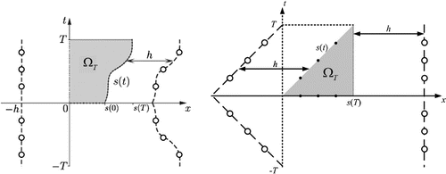
By ‘minimal’, we mean that the position of source and collocation points are taken in the sense of [8,9]. In the interval [$h_{min},h_{max}$], we choose values for h (the distance of the source points from the boundary) with a step size of $h_{step}$. For each such value of h and fixed $\mathcal{N}$, we solve the system (15(15) $$\begin{array}{c}\hfill (A^{T}A+\mathit{\lambda }I)c=A^{T}g,\end{array}$$(15) ) for each value of $\mathit{\lambda }$ ranging between ${\mathit{\lambda }}_{min}$ to ${\mathit{\lambda }}_{max}$ with an increment of ${\mathit{\lambda }}_{step}$. Thus, we obtain c by solving the system (15(15) $$\begin{array}{c}\hfill (A^{T}A+\mathit{\lambda }I)c=A^{T}g,\end{array}$$(15) ), noting the fact that we add $\mathit{\delta }$% of relative random noise to the known boundary data $g_0(t)$.

Using this value of c, we compute the MFS approximation $u_{MFS}^{\mathit{\delta }}$ and consequently, we estimate the absolute maximum error $e_{max}^{\mathit{\delta }}={max}_{{\overline{\mathrm{\Omega }}}_T}|u_{MFS}^{\mathit{\delta }}-u|$, where u is the exact solution. We call $e_{max,opt}^{\mathit{\delta },loc,\mathit{\lambda }}$, the minimum of all such values of $e_{max}^{\mathit{\delta }}$ for fixed values of $\mathcal{N}$, h, $\mathit{\delta }$ and varying $\mathit{\lambda }$. Furthermore, for fixed values of $\mathcal{N}$ and $\mathit{\delta }$, we call the minimum of $e_{max,opt}^{\mathit{\delta },loc,\mathit{\lambda }}$, for all values of h between $h_{min}$ to $h_{max}$ with an increment of $h_{step}$, as $e_{max,opt}^{\mathit{\delta },loc,\mathit{\lambda },h}$.

Thus, calculating $e_{max,opt}^{\mathit{\delta },loc,\mathit{\lambda },h}$, we check whether we attained the desired accuracy Tol, i.e. $e_{max,opt}^{\mathit{\delta },loc,\mathit{\lambda },h}<Tol$. We mark that value of $e_{max,opt}^{\mathit{\delta },loc,\mathit{\lambda },h}$ and store it in a set ${\mathcal{S}}_{opt}$.

Case I: ${\mathcal{S}}_{opt}\ne \mathrm{\varnothing }$ signifies that the desired accuracy on the absolute error on the entire domain (hence, the accuracy of Dirichlet data) is attained. Then we call stored singleton element in ${\mathcal{S}}_{opt}$ as $e_{max,opt}^{\mathit{\delta }}$. The values of h and $\mathcal{N}$ corresponding to which $e_{max,opt}^{\mathit{\delta }}$ is attained will give the optimal location and minimum value of $\mathcal{N}$.

Case II: If ${\mathcal{S}}_{opt}=\mathrm{\varnothing }$, we move to the next iteration, where we increase the number of collocation and source points to get a better MFS approximation and repeat the same process.

The significance of this algorithm in terms of the overall computational time for solving the overall inverse problem should be appreciated. The algorithm is meant to find the ($h,\mathcal{N},\mathit{\lambda }$)-combination which finds u optimally to within a prescribed tolerance, Tol,  for a certain level of random noise, $\mathit{\delta }.$ We seek $\mathcal{N}$ as small as possible, since it is this parameter that affects the computational time required to find u the most. However, the value of $\mathcal{N}$ is affected by the values of h and $\mathit{\lambda }$ that are chosen, which is why we need to optimize for ($h,\mathcal{N},\mathit{\lambda }$). Having understood this, a subsidiary issue is the computational time required to find the optimal ( $h,N,\mathit{\lambda }$ ); is there some way to optimize this? We have not tackled this explicitly, but our algorithm at least provides a simple and rational, if not necessarily optimal, way to find the optimal ($h,\mathcal{N},\mathit{\lambda }$)-combination. We can note in this context that this is the first time that an attempt has been made to find all three parameters simultaneously; for example, in [9], only $\mathit{\lambda }$ is optimized for. Further remarks on the computational expense associated with the algorithm are given in Remark 4 in Section 4.

4. Numerical investigations

In this section, we investigated three benchmark problems to demonstrate the effectiveness of our proposed algorithm. We tested all the benchmark problems with our algorithm several times with input data as ${\mathcal{N}}_0=4$, $h_{min}=1$, $h_{step}=0.1$, $h_{max}=3.5$, ${\mathit{\lambda }}_{min}={10}^{-16}$, ${\mathit{\lambda }}_{step}={10}^1$ and ${\mathit{\lambda }}_{max}={10}^{-1}$. Previous MFS investigations [8,9] indicate that a reasonable value for the parameter $h>0$ has to be chosen neither too close (where near singularities of the fundamental solution become visible), nor too far away (where the instabilities caused by increasing ill-conditioning start to manifest themselves) from the domain (0, s(t)). Hence, it makes the choices of $h_{min}=1$ and $h_{max}=3.5$ quite reasonable. The effect of $\mathit{\delta }$ and accuracy Tol on the placement and number of source points is shown for each of the examples. To check the effect of the noise and accuracy on $h_{opt}$ and ${\mathcal{N}}_{opt}$, we considered four different cases. Results are observed by taking $\mathit{\delta }=5\%$ in cases (a), (b) and $\mathit{\delta }=1\%$ in cases (c), (d) and by allowing the accuracy to vary. Similarly, in cases (a) and (c), results are observed under a fixed accuracy ($Tol=0.1$) but allowing $\mathit{\delta }$ to vary. In cases (b) and (d), both Tol and $\mathit{\delta }$ are allowed to vary. Once we have obtained $h_{opt}$ and ${\mathcal{N}}_{opt}$ using our algorithm, we applied ten sets of random data to produce the plots.

The benchmark problems are chosen in such a way that an analytical solution u(x, t) and the location of the moving boundary s(t) are known. In the first and third examples, we will have s(t) as a linear function of t, whereas in the second example we will have s(t) as a nonlinear function of t. In all the examples, random noise will be applied to the interface Neumann condition (5(5) $$\begin{array}{cc}\hfill \frac{\mathit{\partial }u}{\mathit{\partial }x}(s(t),t)& =h_2(t),t\in (0,T],\hfill \end{array}$$(5) ). Noise could also be added to some other quantity related to the position of the moving boundary s(t) [26], but this case is not pursued herein.

For the purposes of comparison, we considered the first two examples that were investigated in [9]. The third example is the classical problem of ablation, posed on a shrinking domain.

4.1. Example 1

We start with an example for which the exact solution is given by(16) $$\begin{array}{c}\hfill u(x,t)=-1+exp(1-\frac{1}{\sqrt{2}}+\frac{t}{\sqrt{2}}-\frac{x}{\sqrt{2}}),(x,t)\in [0,s(t)]\times [0,T]\end{array}$$(16)

along with the moving boundary given by the linear function(17) $$\begin{array}{c}\hfill s(t)=\sqrt{2}-1+\frac{t}{\sqrt{2}},t\in [0,T],\end{array}$$(17)

where $T=1$. Thus, for this example we have the following initial condition(18) $$\begin{array}{c}\hfill u(x,0)=-1+exp(1-\frac{1}{\sqrt{2}}-\frac{x}{\sqrt{2}}),x\in [0,s(0)],s(0)=\sqrt{2}-1,\end{array}$$(18)

and interface boundary conditions(19) $$\begin{array}{cc}\hfill u(s(t),t)& =0,t\in (0,1],\hfill \end{array}$$(19) (20) $$\begin{array}{cc}\hfill \frac{\mathit{\partial }u}{\mathit{\partial }x}(s(t),t)& =-\frac{\mathrm{d}s}{\mathrm{d}t}=-\frac{1}{\sqrt{2}}.\hfill \end{array}$$(20) Random noise is added to the Neumann data (20(20) $$\begin{array}{cc}\hfill \frac{\mathit{\partial }u}{\mathit{\partial }x}(s(t),t)& =-\frac{\mathrm{d}s}{\mathrm{d}t}=-\frac{1}{\sqrt{2}}.\hfill \end{array}$$(20) ) in the form(21) $$\begin{array}{c}\hfill u_x^{\mathit{\delta }}(s(t,t))=-\frac{1}{\sqrt{2}}+N(0,{\mathit{\sigma }}^2),\end{array}$$(21)

where $N(0,{\mathit{\sigma }}^2)$ represents the normal distribution with mean zero and standard deviation(22) $$\begin{array}{c}\hfill \mathit{\sigma }=\mathit{\delta }\times \underset{(s(t),t),t\in (0,1]}{max}|u_x(s(t),t)|=\frac{\mathit{\delta }}{\sqrt{2}}.\end{array}$$(22)

We wish to recover the Dirichlet and Neumann boundary conditions along the fixed boundary $x=0$ given by(23) $$\begin{array}{c}\hfill u(0,t)=-1+exp(1-\frac{1}{\sqrt{2}}+\frac{t}{2}),\frac{\mathit{\partial }u}{\mathit{\partial }x}(0,t)=-\frac{1}{\sqrt{2}}exp(1-\frac{1}{\sqrt{2}}+\frac{t}{2}).\end{array}$$(23)

For the placement of source and collocation points, we refer to subsection 2.2.

Case (a): Tol = 0.1, $\mathit{\delta }$ = 5%

Successive application of our algorithm yields the output as $h_{opt}=2.5,2.4$ with ${\mathcal{N}}_{opt}=8$. In Figure 2, the first plot shows the L-curve for 5% of random noise at $h=2.5$ with $\mathcal{N}=8$, whereas the absolute error for all $(x,t)\in {\mathrm{\Omega }}_T$ for the noise level $\mathit{\delta }=5\%$ at $h=2.5$, $\mathcal{N}=8$ and with $\mathit{\lambda }={10}^{-6}$, which corresponds to the corner of the L-curve, is shown in the three-dimensional plot on the right. Similar plots have been shown in Figure 4 for $h=2.4$, $\mathcal{N}=8$ and $\mathit{\lambda }={10}^{-6}$. The MFS approximations for u(0, t) and $u_x(0,t)$ for $\mathit{\delta }=5\%$, $\mathcal{N}=8$, $\mathit{\lambda }={10}^{-6}$ at $h=2.5$ are plotted in Figure 3, whereas the corresponding approximations for $\mathit{\delta }=5\%$, $\mathcal{N}=8$, $\mathit{\lambda }={10}^{-6}$ at $h=2.4$ are plotted in Figure 5.

Figure 2. Case (a) of Example 1: The first plot shows the L-curve for $\mathit{\delta }=5\%$, $h=2.5$ and $\mathcal{N}=8$. The second plot shows the absolute error on the entire domain for $\mathit{\delta }=5\%$, $h=2.5$, $\mathcal{N}=8$ and $\mathit{\lambda }={10}^{-6}$. The corresponding root-mean-square error (RMSE) over the entire domain is 0.0188106.

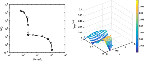
Figure 3. Case (a) of Example 1: The first plot shows the reconstructed Dirichlet data at $x=0$ for $\mathit{\delta }=5\%$, $h=2.5$, $\mathcal{N}=8$ and $\mathit{\lambda }={10}^{-6}$. The second plot shows the reconstructed Neumann data at $x=0$ for $\mathit{\delta }=5\%$, $h=2.5$, $\mathcal{N}=8$ and $\mathit{\lambda }={10}^{-6}$.

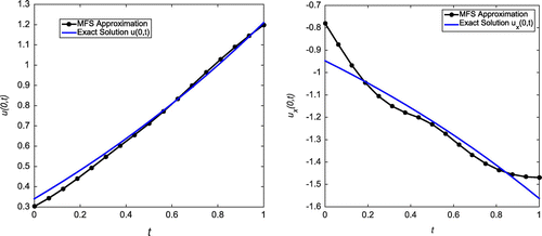
Figure 4. Case (a) of Example 1: The first plot shows the L-curve for $\mathit{\delta }=5\%$, $h=2.4$ and $\mathcal{N}=8$. The second plot shows the absolute error on the entire domain for $\mathit{\delta }=5\%$, $h=2.4$, $\mathcal{N}=8$ and $\mathit{\lambda }={10}^{-6}$. The corresponding RMSE over the entire domain is 0.0180478.

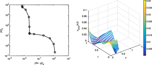
Figure 5. Case (a) of Example 1: The first plot shows the reconstructed Dirichlet data at $x=0$ for $\mathit{\delta }=5\%$, $h=2.4$, $\mathcal{N}=8$ and $\mathit{\lambda }={10}^{-6}$. The second plot shows the reconstructed Neumann data at $x=0$ for $\mathit{\delta }=5\%$, $h=2.4$, $\mathcal{N}=8$ and $\mathit{\lambda }={10}^{-6}$.

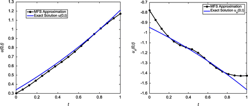
Case (b): Tol = 0.04, $\mathit{\delta }$ = 5%

In this case, our algorithm predicts the output as $h_{opt}=2.9$ with ${\mathcal{N}}_{opt}=12$. The first plot of Figure 6 shows the L-curve for 5% of random noise, where source points have been placed with $h=2.9$, $\mathcal{N}=12$. The second plot refers to a three-dimensional plot of the absolute error for all $(x,t)\in {\mathrm{\Omega }}_T$ for the noise level $\mathit{\delta }=5\%$ at $h=2.9$, $\mathcal{N}=12$ and with $\mathit{\lambda }={10}^{-7}$, which corresponds to the corner of the L-curve. The MFS approximations for u(0, t) and $u_x(0,t)$ are plotted for 5% noise level in Figure 7.

Figure 6. Case (b) of Example 1: The first plot shows the L-curve for $\mathit{\delta }=5\%$, $h=2.9$ and $\mathcal{N}=12$. The second plot shows the absolute error on the entire domain for $\mathit{\delta }=5\%$, $h=2.9$, $\mathcal{N}=12$ and $\mathit{\lambda }={10}^{-7}$. The corresponding RMSE over the entire domain is 0.00822492.

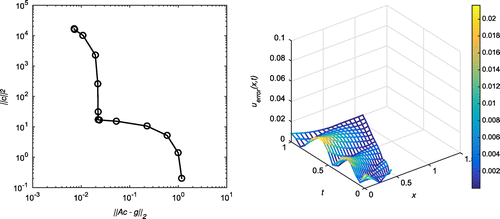
Figure 7. Case (b) of Example 1: The first plot shows the reconstructed Dirichlet data at $x=0$ for $\mathit{\delta }=5\%$, $h=2.9$, $\mathcal{N}=12$ and $\mathit{\lambda }={10}^{-7}$. The second plot shows the reconstructed Neumann data at $x=0$ for $\mathit{\delta }=5\%$, $h=2.9$, $\mathcal{N}=12$ and $\mathit{\lambda }={10}^{-7}$. We observe that the results generated from Johansson et al. [9] have used $\mathcal{N}=124$ compared to our results which have been obtained using just $\mathcal{N}=12$.

Case (c): Tol = 0.1, $\mathit{\delta }$ = 1%

In this case, our algorithm predicts the output as $h_{opt}=1.6$ with ${\mathcal{N}}_{opt}=8$. The first plot of Figure 8 shows the L-curve for 1% of random noise, where source points have been placed with $h=1.6$, $\mathcal{N}=8$. The second plot shows the absolute error for all $(x,t)\in {\mathrm{\Omega }}_T$ for the noise level $\mathit{\delta }=1\%$ at $h=1.6$, $\mathcal{N}=8$ and with $\mathit{\lambda }={10}^{-9}$, which corresponds to the corner of the L-curve. The MFS approximations for u(0, t) and $u_x(0,t)$ are plotted for 1% noise level in Figure 9.

Figure 8. Case (c) of Example 1: The first plot shows the L-curve for $\mathit{\delta }=1\%$, $h=1.6$ and $\mathcal{N}=8$. The second plot shows the absolute error on the entire domain for $\mathit{\delta }=1\%$, $h=1.6$, $\mathcal{N}=8$ and $\mathit{\lambda }={10}^{-9}$. The corresponding RMSE over the entire domain is 0.0196486.

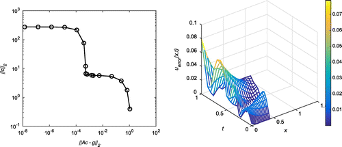
Figure 9. Case (c) of Example 1: The first plot shows the reconstructed Dirichlet data at $x=0$ for $\mathit{\delta }=1\%$, $h=1.6$, $\mathcal{N}=8$ and $\mathit{\lambda }={10}^{-9}$. The second plot shows the reconstructed Neumann data at $x=0$ for $\mathit{\delta }=1\%$, $h=1.6$, $\mathcal{N}=8$ and $\mathit{\lambda }={10}^{-9}$.

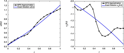
Case (d): Tol = 0.01, $\mathit{\delta }$ = 1%

Successive application of our algorithm yields the output as $h_{opt}=2.7$ with ${\mathcal{N}}_{opt}=16$ and $h_{opt}=3.1$ with ${\mathcal{N}}_{opt}=20$. In Figure 10, the first plot shows the L-curve for 1% of random noise at $h=2.7$ with $\mathcal{N}=16$, whereas the absolute error for all $(x,t)\in {\mathrm{\Omega }}_T$ for the noise level $\mathit{\delta }=1\%$ at $h=2.7$, $\mathcal{N}=16$ and with $\mathit{\lambda }={10}^{-10}$ is shown in the second plot. Similar plots have been shown in Figure 12 for $h=3.1$, $\mathcal{N}=20$ and $\mathit{\lambda }={10}^{-11}$. The MFS approximations for u(0, t) and $u_x(0,t)$ for $\mathit{\delta }=1\%$, $\mathcal{N}=16$, $\mathit{\lambda }={10}^{-10}$ at $h=2.7$ are plotted in Figure 11, and corresponding approximations for $\mathit{\delta }=1\%$, $\mathcal{N}=20$, $\mathit{\lambda }={10}^{-11}$ at $h=3.1$ are plotted in Figure 13.

Figure 10. Case (d) of Example 1: The first plot shows the L-curve for $\mathit{\delta }=1\%$, $h=2.7$ and $\mathcal{N}=16$. The second plot shows the absolute error on the entire domain for $\mathit{\delta }=1\%$, $h=2.7$, $\mathcal{N}=16$ and $\mathit{\lambda }={10}^{-10}$. The corresponding RMSE over the entire domain is 0.00164797.

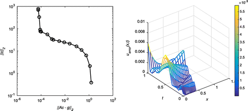
Figure 11. Case (d) of Example 1: The first plot shows the reconstructed Dirichlet data at $x=0$ for $\mathit{\delta }=1\%$, $h=2.7$, $\mathcal{N}=16$ and $\mathit{\lambda }={10}^{-10}$. The second plot shows the reconstructed Neumann data at $x=0$ for $\mathit{\delta }=1\%$, $h=2.7$, $\mathcal{N}=16$ and $\mathit{\lambda }={10}^{-10}$. We observe that the results generated from Johansson et al. [9] have used $\mathcal{N}=124$ compared to our results which have been obtained using just $\mathcal{N}=16$.

Figure 12. Case (d) of Example 1: The first plot shows the L-curve for $\mathit{\delta }=1\%$, $h=3.1$ and $\mathcal{N}=20$. The second plot shows the absolute error on the entire domain for $\mathit{\delta }=1\%$, $h=3.1$, $\mathcal{N}=20$ and $\mathit{\lambda }={10}^{-11}$. The corresponding RMSE over the entire domain is 0.00198483.

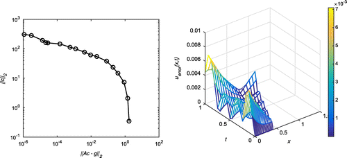
Figure 13. Case (d) of Example 1: The first plot shows the reconstructed Dirichlet data at $x=0$ for $\mathit{\delta }=1\%$, $h=3.1$, $\mathcal{N}=20$ and $\mathit{\lambda }={10}^{-11}$. The second plot shows the reconstructed Neumann data at $x=0$ for $\mathit{\delta }=1\%$, $h=3.1$, $\mathcal{N}=20$ and $\mathit{\lambda }={10}^{-11}$. We observe that the results generated from Johansson et al. [9] have used $\mathcal{N}=124$ compared to our results which have been obtained using just $\mathcal{N}=20$.

Observations

In cases (a) and (c), we are concerned with $O({10}^{-2})$ accuracy for $\mathit{\delta }=5\%,1\%$, respectively. We observe that the MFS approximations for u(0, t) and $u_x(0,t)$, respectively, match well with the exact solution and are similar to [9] in cases (a) and (c). However, we note that our results are produced through 8 source and 8 collocation points compared to [9], where the authors have used 64 source and 64 collocation points to produce similar results. Moreover, in [9] the authors have increased the number of source and collocation points to 124 to check whether the results can be improved and they have found that the results (see Figures 6 and 8 in [9]) are not improved significantly. On the contrary, on reducing the Tol value in our algorithm in cases (b) ($\mathit{\delta }=5\%$) and (d) ($\mathit{\delta }=1\%$), our results improve significantly. In fact, we found that one can get $O({10}^{-3})$ results (see Figures 10 and 12) even when we applied an error of $O({10}^{-2})$ on the Neumann boundary condition for $\mathit{\delta }=1\%$. This is noteworthy, as we have used only comparatively few collocation and source points, 16 and 20 respectively, to obtain such results. In fact, one cannot distinguish the MFS approximations for u(0, t) and the exact solution, as is evident from the left-hand plots of Figures 11 and 13). A greater accuracy is attained for $u_x(0,t)$ (see the right hand side plots of the Figures 11 and 13) as compared to [9]. An exception occurs: as t increases, the accuracy does not decrease [9]. However, this is not the case with $\mathit{\delta }=5\%$, i.e. for a reasonably large amount of noise. We obtain $O({10}^{-2})$ results, as seen in Figure 6 when applying an error of $O({10}^{-2})$ on the Neumann boundary condition for $\mathit{\delta }=5\%$. However, we want to comment that one could increase the accuracy up to a certain degree using our algorithm, but not up to $O({10}^{-3})$ (see second plot of Figure 6) when applying an error of $O({10}^{-2})$ on the Neumann boundary condition in the case of $\mathit{\delta }=5\%$.

4.2. Example 2

This example concerns a problem where the moving boundary is given by a nonlinear function. In this example, the exact solution is given by(24) $$\begin{array}{c}\hfill u(x,t)=-\frac{x^2}{2}+2x-\frac{1}{2}-t,(x,t)\in [0,s(t)]\times [0,T]\end{array}$$(24)

along with the nonlinear moving boundary given by(25) $$\begin{array}{c}\hfill s(t)=2-\sqrt{3-2t},t\in [0,T],\end{array}$$(25)

where $T=1$. Thus, the initial and interface boundary conditions are given by:(26) $$\begin{array}{cc}\hfill u(x,0)& =-\frac{x^2}{2}+2x-\frac{1}{2},x\in [0,s(0)],s(0)=2-\sqrt{3},\hfill \end{array}$$(26) (27) $$\begin{array}{cc}\hfill u(s(t),t)& =0,t\in (0,1],\hfill \end{array}$$(27) (28) $$\begin{array}{cc}\hfill \frac{\mathit{\partial }u}{\mathit{\partial }x}(s(t),t)& =\sqrt{3-2t},t\in (0,1].\hfill \end{array}$$(28)

We observe that the Neumann boundary condition (28(28) $$\begin{array}{cc}\hfill \frac{\mathit{\partial }u}{\mathit{\partial }x}(s(t),t)& =\sqrt{3-2t},t\in (0,1].\hfill \end{array}$$(28) ) is not given by the classical Stefan boundary condition, but rather by a more general boundary condition (5(5) $$\begin{array}{cc}\hfill \frac{\mathit{\partial }u}{\mathit{\partial }x}(s(t),t)& =h_2(t),t\in (0,T],\hfill \end{array}$$(5) ). For the placement of source and collocation points, we refer to subsection 2.2 with the following modification to the second equation in (11(11) $$\begin{array}{cc}\hfill u_M(x_1^i,t_i)& =0,\frac{\mathit{\partial }{u}_M}{\mathit{\partial }x}(x_1^i,t_i)=-s^{\prime }(t_i),i=0,\dots ,M.\hfill \end{array}$$(11) ):(29) $$\begin{array}{c}\hfill \frac{\mathit{\partial }u}{\mathit{\partial }x}(x_1^i,t_i)=\sqrt{3-2t_i},i=0,1,\dots ,M.\end{array}$$(29)

Random noise is added to the interface Neumann boundary condition, and (28(28) $$\begin{array}{cc}\hfill \frac{\mathit{\partial }u}{\mathit{\partial }x}(s(t),t)& =\sqrt{3-2t},t\in (0,1].\hfill \end{array}$$(28) ) has been included as(30) $$\begin{array}{c}\hfill u_x^{\mathit{\delta }}(s(t,t))=\sqrt{3-2t}+N(0,{\mathit{\sigma }}^2),\end{array}$$(30)

where(31) $$\begin{array}{c}\hfill \mathit{\sigma }=\mathit{\delta }\times \underset{(s(t),t),t\in (0,1]}{max}|u_x(s(t),t)|=\sqrt{3}\mathit{\delta }.\end{array}$$(31)

The Dirichlet and Neumann boundary conditions to be recovered along the fixed boundary at $x=0$ are given by(32) $$\begin{array}{cc}\hfill u(0,t)=-\frac{1}{2}-t,\frac{\mathit{\partial }u}{\mathit{\partial }x}(0,t)& =2,t\in [0,1].\hfill \end{array}$$(32) Case (a): Tol = 0.1, $\mathit{\delta }$ = 5%

Successive application of our algorithm yields the output as $h_{opt}=2.3,2.4$ with ${\mathcal{N}}_{opt}=8$. In Figure 14, the first plot shows the L-curve for 5% of random noise at $h=2.3$ with $\mathcal{N}=8$, whereas the absolute error for all $(x,t)\in {\mathrm{\Omega }}_T$ for the noise level $\mathit{\delta }=5\%$ at $h=2.3$, $\mathcal{N}=8$ and with $\mathit{\lambda }={10}^{-6}$, which corresponds to the corner of the L-curve, is shown in the second plot. Similar plots have been shown in Figure 16 for $h=2.4$, $\mathcal{N}=8$ and $\mathit{\lambda }={10}^{-6}$. The MFS approximations for u(0, t) and $u_x(0,t)$ for $\mathit{\delta }=5\%$, $\mathcal{N}=8$, $\mathit{\lambda }={10}^{-6}$ and $h=2.3$ are plotted in Figure 15 and the corresponding approximations for $\mathit{\delta }=5\%$, $\mathcal{N}=8$, $\mathit{\lambda }={10}^{-6}$ and $h=2.4$ are plotted in Figure 17.

Figure 14. Case (a) of Example 2: The first plot shows the L-curve for $\mathit{\delta }=5\%$, $h=2.3$ and $\mathcal{N}=8$. The second plot shows the absolute error on the entire domain for $\mathit{\delta }=5\%$, $h=2.3$, $\mathcal{N}=8$ and $\mathit{\lambda }={10}^{-6}$. The corresponding RMSE over the entire domain is 0.0317699.

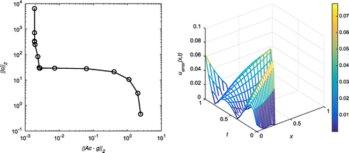
Figure 15. Case (a) of Example 2: The first plot shows the reconstructed Dirichlet data at $x=0$ for $\mathit{\delta }=5\%$, $h=2.3$, $\mathcal{N}=8$ and $\mathit{\lambda }={10}^{-6}$. The second plot shows the reconstructed Neumann data at $x=0$ for $\mathit{\delta }=5\%$, $h=2.3$, $\mathcal{N}=8$ and $\mathit{\lambda }={10}^{-6}$.

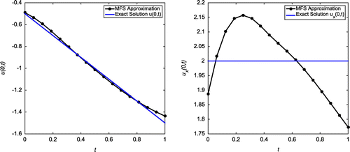
Figure 16. Case (a) of Example 2: The first plot shows the L-curve for $\mathit{\delta }=5\%$, $h=2.4$ and $\mathcal{N}=8$. The second plot shows the absolute error on the entire domain for $\mathit{\delta }=5\%$, $h=2.4$, $\mathcal{N}=8$ and $\mathit{\lambda }={10}^{-6}$. The corresponding RMSE over the entire domain is 0.0394105.

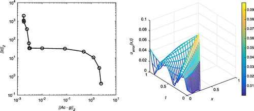
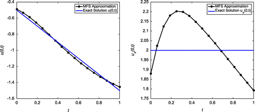
Figure 17. Case (a) of Example 2: The first plot shows the reconstructed Dirichlet data at $x=0$ for $\mathit{\delta }=5\%$, $h=2.4$, $\mathcal{N}=8$ and $\mathit{\lambda }={10}^{-6}$. The second plot shows the reconstructed Neumann data at $x=0$ for $\mathit{\delta }=5\%$, $h=2.4$, $\mathcal{N}=8$ and $\mathit{\lambda }={10}^{-6}$.

Case (b): Tol = 0.05, $\mathit{\delta }$ = 5%

In this case, our algorithm predicts the output as $h_{opt}=2.3$ with ${\mathcal{N}}_{opt}=12$. The first plot of Figure 18 shows the L-curve for 5% of random noise, where source points have been placed with $h=2.3$, $\mathcal{N}=12$. The second plot shows the absolute error for all $(x,t)\in {\mathrm{\Omega }}_T$ for the noise level $\mathit{\delta }=5\%$ at $h=2.3$, $\mathcal{N}=12$ and with $\mathit{\lambda }={10}^{-6}$, which corresponds to the corner of the L-curve. The MFS approximations for u(0, t) and $u_x(0,t)$ are plotted for 5% noise level in Figure 19.

Figure 18. Case (b) of Example 2: The first plot shows the L-curve for $\mathit{\delta }=5\%$, $h=2.3$ and $\mathcal{N}=12$. The second plot shows the absolute error on the entire domain for $\mathit{\delta }=5\%$, $h=2.3$, $\mathcal{N}=12$ and $\mathit{\lambda }={10}^{-6}$. The corresponding RMSE over the entire domain is 0.013304.

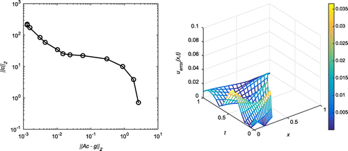
Figure 19. Case (b) of Example 2: The first plot shows the reconstructed Dirichlet data at $x=0$ for $\mathit{\delta }=5\%$, $h=2.3$, $\mathcal{N}=12$ and $\mathit{\lambda }={10}^{-6}$. The second plot shows the reconstructed Neumann data at $x=0$ for $\mathit{\delta }=5\%$, $h=2.3$, $\mathcal{N}=12$ and $\mathit{\lambda }={10}^{-6}$. We observe that the results generated from Johansson et al. [9] have used $\mathcal{N}=64$ compared to our results which have been obtained using just $\mathcal{N}=12$.

Case (c): Tol = 0.1, $\mathit{\delta }$ = 1%

In this case, our algorithm predicts the output as $h_{opt}=1.8$ with ${\mathcal{N}}_{opt}=8$. The first plot of Figure 20 shows the L-curve for 1% of random noise, where source points have been placed with $h=1.8$, $\mathcal{N}=8$. The second plot shows the absolute error for all $(x,t)\in {\mathrm{\Omega }}_T$ for the noise level $\mathit{\delta }=1\%$ at $h=1.8$, $\mathcal{N}=8$ and with $\mathit{\lambda }={10}^{-9}$, which corresponds to the corner of the L-curve. The MFS approximations for u(0, t) and $u_x(0,t)$ are plotted for 1% noise level in Figure 21.

Figure 20. Case (c) of Example 2: The first plot shows the L-curve for $\mathit{\delta }=1\%$, $h=1.8$ and $\mathcal{N}=8$. The second plot shows the absolute error on the entire domain for $\mathit{\delta }=1\%$, $h=1.8$, $\mathcal{N}=8$ and $\mathit{\lambda }={10}^{-9}$. The corresponding RMSE over the entire domain is 0.0220787.

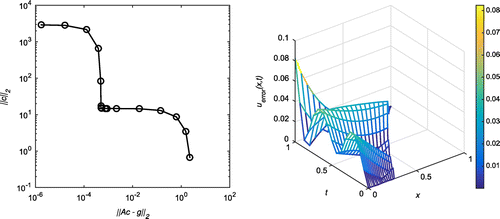
Figure 21. Case (c) of Example 2: The first plot shows the reconstructed Dirichlet data at $x=0$ for $\mathit{\delta }=1\%$, $h=1.8$, $\mathcal{N}=8$ and $\mathit{\lambda }={10}^{-9}$. The second plot shows the reconstructed Neumann data at $x=0$ for $\mathit{\delta }=1\%$, $h=1.8$, $\mathcal{N}=8$ and $\mathit{\lambda }={10}^{-9}$.

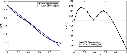
Case (d): Tol = 0.01, $\mathit{\delta }$ = 1%

In this case, our algorithm predicts the output as $h_{opt}=2.2$ with ${\mathcal{N}}_{opt}=20$. The first plot of Figure 22 shows the L-curve for 1% of random noise, where source points have been placed with $h=2.2$, $\mathcal{N}=20$. The second plot shows the absolute error for all $(x,t)\in {\mathrm{\Omega }}_T$ for the noise level $\mathit{\delta }=1\%$ at $h=2.2$, $\mathcal{N}=20$ and with $\mathit{\lambda }={10}^{-9}$, which corresponds to the corner of the L-curve. The MFS approximations for u(0, t) and $u_x(0,t)$ are plotted for 1% noise level in Figure 23.

Figure 22. Case (d) of Example 2: The first plot shows the L-curve for $\mathit{\delta }=1\%$, $h=2.2$ and $\mathcal{N}=20$. The second plot shows the absolute error on the entire domain for $\mathit{\delta }=1\%$, $h=2.2$, $\mathcal{N}=20$ and $\mathit{\lambda }={10}^{-9}$. The corresponding RMSE over the entire domain is 0.00254839.

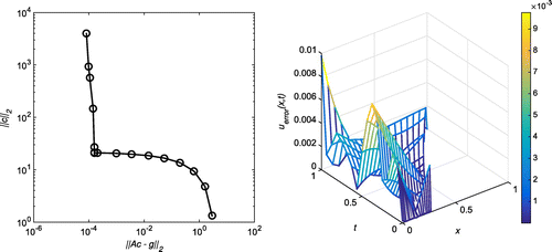
Figure 23. Case (d) of Example 2: The first plot shows the reconstructed Dirichlet data at $x=0$ for $\mathit{\delta }=1\%$, $h=2.2$, $\mathcal{N}=20$ and $\mathit{\lambda }={10}^{-9}$. The second plot shows the reconstructed Neumann data at $x=0$ for $\mathit{\delta }=1\%$, $h=2.2$, $\mathcal{N}=20$ and $\mathit{\lambda }={10}^{-9}$. We observe that the results generated from Johansson et al. [9] have used $\mathcal{N}=64$ compared to our results which have been obtained using just $\mathcal{N}=20$.

Observations

In cases (a) and (c), we are concerned with $O({10}^{-2})$ accuracy for $\mathit{\delta }=5\%,1\%$, respectively. We observe that the MFS approximations for u(0, t) and $u_x(0,t)$, respectively, match well with the exact solution and are similar to [9] in cases (a) and (c). As before, we note that our results are produced using 8 source and 8 collocation points compared to [9], where 64 source and 64 collocation points were used to produce similar results. As before, by reducing the Tol value in our algorithm in cases (b) ($\mathit{\delta }=5\%$) and (d) ($\mathit{\delta }=1\%$), our results improve significantly. We can obtain $O({10}^{-3})$ results (see Figure 22) even when applying an error of $O({10}^{-2})$ on the Neumann boundary condition for $\mathit{\delta }=1\%$. Only 20 collocation and source points are used to obtain such results. In this example also, one cannot distinguish the MFS approximations for u(0, t) and the exact solution, as is seen in the first plot of Figure 23. There is a notable observation regarding the accuracy of $u_x(0,t)$ (see the right hand side plot of the Figure 19) as compared to [9]. However, this is not the case with $\mathit{\delta }=5\%$ (reasonably large amount of noise). We obtain $O({10}^{-2})$ results (see Figure 6) when applying an error of $O({10}^{-2})$ on the Neumann boundary condition for $\mathit{\delta }=5\%$. As in Example 1, we want to comment that one can increase the accuracy up to certain degree using our algorithm, but not up to $O({10}^{-3})$ (see Figure 18) when we apply an error of $O({10}^{-2})$ on the Neumann boundary condition in the case of $\mathit{\delta }=5\%$.

4.3. Example 3

The next example is associated with ablation, which is the generic term used for the removal of material from the surface of an object by vaporization, chipping, or other erosive processes [27]. Ablation occurs in spaceflight during atmospheric reentry [28], the burning up of meteorites [29], the melting or sublimation of a solid [30], laser drilling in metals and the cornea [31], the reduction of glaciers by erosion [32] and the surgical removal of a body part or tissue, such as in atrial fibrillation [33]. In mathematical terms, ablation is one type of phase-change, or Stefan problem in which the location of the surface of the ablating material is not known beforehand, but must be determined as part of the solution.

A significant difference between the two earlier examples and this one is that in the former, the extent of the solution domain grows with time, whereas for the latter it decreases; thus, a different distribution of source and collocation points is appropriate.

The exact solution is given by(33) $$\begin{array}{c}\hfill u(x,t)=-1+exp(t-x),(x,t)\in [0,1]\times [0,T]\end{array}$$(33)

along with the linear moving boundary given by(34) $$\begin{array}{c}\hfill s(t)=t,t\in [0,T],\end{array}$$(34)

where $T=1$. The interface boundary conditions are given by:(35) $$\begin{array}{cc}\hfill u(s(t),t)& =0,t\in (0,1],\hfill \end{array}$$(35) (36) $$\begin{array}{cc}\hfill \frac{\mathit{\partial }u}{\mathit{\partial }x}(s(t),t)& =-\frac{\mathrm{d}s}{\mathrm{d}t}=-1.\hfill \end{array}$$(36)

Random noise is added to the interface Neumann condition (36(36) $$\begin{array}{cc}\hfill \frac{\mathit{\partial }u}{\mathit{\partial }x}(s(t),t)& =-\frac{\mathrm{d}s}{\mathrm{d}t}=-1.\hfill \end{array}$$(36) ) in the form(37) $$\begin{array}{c}\hfill u_x^{\mathit{\delta }}(s(t,t))=-1+N(0,{\mathit{\sigma }}^2),\end{array}$$(37)

where $N(0,{\mathit{\sigma }}^2)$ represents the normal distribution with mean zero and standard deviation(38) $$\begin{array}{c}\hfill \mathit{\sigma }=\mathit{\delta }\times \underset{(s(t),t),t\in (0,1]}{max}|u_x(s(t),t)|=\mathit{\delta }.\end{array}$$(38)

We wish to recover the Dirichlet and Neumann boundary conditions along the fixed boundary $x=1$ given by(39) $$\begin{array}{c}\hfill u(1,t)=-1+exp(t-1),\frac{\mathit{\partial }u}{\mathit{\partial }x}(1,t)=-exp(t-1).\end{array}$$(39)

For the placement of source and collocation points, we refer to subsection 2.2.

Case (a): Tol = 0.1, $\mathit{\delta }$ = 5%

Successive application of our algorithm yields the output as $h_{opt}=1.8,1.7$ with ${\mathcal{N}}_{opt}=8$. In Figure 24, the first plot shows the L-curve for 5% of random noise at $h=1.8$ with $\mathcal{N}=8$, whereas a three-dimensional plot of the absolute error for all $(x,t)\in {\mathrm{\Omega }}_T$ for the noise level $\mathit{\delta }=5\%$ at $h=1.8$, $\mathcal{N}=8$ and with $\mathit{\lambda }={10}^{-5}$ is shown on the right. We note that, here, the curve does not really have the usual L-shape due to the fact that any value of $\mathit{\lambda }\le {10}^{-5}$ seems to yield an optimal choice of regularization parameter. Similar plots have been shown in Figure 26 for $h=1.7$, $\mathcal{N}=8$ and $\mathit{\lambda }={10}^{-5}$. 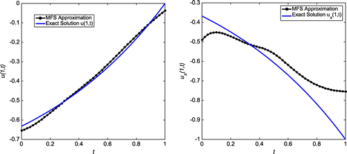The MFS approximations for u(1, t) and $u_x(1,t)$ for $\mathit{\delta }=5\%$, $\mathcal{N}=8$, $\mathit{\lambda }={10}^{-5}$ at $h=1.8$ are plotted in Figure 25 and the corresponding approximations for $\mathit{\delta }=5\%$, $\mathcal{N}=8$, $\mathit{\lambda }={10}^{-5}$ at $h=1.7$ are plotted in Figure 27.

Figure 24. Case (a) of Example 3: The first plot shows the L-curve for $\mathit{\delta }=5\%$, $h=1.8$ and $\mathcal{N}=8$. The second plot shows the absolute error on the entire domain for $\mathit{\delta }=5\%$, $h=1.8$, $\mathcal{N}=8$ and $\mathit{\lambda }={10}^{-5}$. The corresponding RMSE over the entire domain is 0.013632.

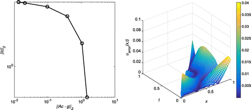
Figure 25. Case (a) of Example 3: The first plot shows the reconstructed Dirichlet data at $x=1$ for $\mathit{\delta }=5\%$, $h=1.8$, $\mathcal{N}=8$ and $\mathit{\lambda }={10}^{-5}$. The second plot shows the reconstructed Neumann data at $x=1$ for $\mathit{\delta }=5\%$, $h=1.8$, $\mathcal{N}=8$ and $\mathit{\lambda }={10}^{-5}$.

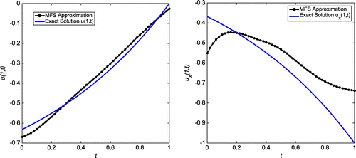
Figure 26. Case (a) of Example 3: The first plot shows the L-curve for $\mathit{\delta }=5\%$, $h=1.7$ and $\mathcal{N}=8$. The second plot shows the absolute error on the entire domain for $\mathit{\delta }=5\%$, $h=1.7$, $\mathcal{N}=8$ and $\mathit{\lambda }={10}^{-5}$. The corresponding RMSE over the entire domain is 0.0175978.

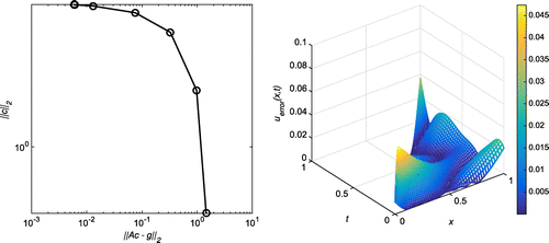
Figure 27. Case (a) of Example 3: The first plot shows the reconstructed Dirichlet data at $x=1$ for $\mathit{\delta }=5\%$, $h=1.7$, $\mathcal{N}=8$ and $\mathit{\lambda }={10}^{-5}$. The second plot shows the reconstructed Neumann data at $x=1$ for $\mathit{\delta }=5\%$, $h=1.7$, $\mathcal{N}=8$ and $\mathit{\lambda }={10}^{-5}$.

Case (b): Tol = 0.04, $\mathit{\delta }$ = 5%

In this case, our algorithm predicts the output as $h_{opt}=2.2$ with ${\mathcal{N}}_{opt}=12$. The first plot of Figure 28 shows the L-curve for 5% of random noise, where source points have been placed with $h=2.2$, $\mathcal{N}=12$. 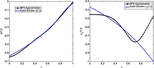The second plot show the absolute error for all $(x,t)\in {\mathrm{\Omega }}_T$ for the noise level $\mathit{\delta }=5\%$ at $h=2.2$, $\mathcal{N}=12$ and with $\mathit{\lambda }={10}^{-7}$, which corresponds to the corner of the L-curve. The MFS approximations for u(1, t) and $u_x(1,t)$ are plotted for a 5% noise level in Figure 29.

Figure 28. The first plot shows the L-curve for $\mathit{\delta }=5\%$, $h=2.2$ and $\mathcal{N}=12$. The second plot shows the absolute error on the entire domain for $\mathit{\delta }=5\%$, $h=2.2$, $\mathcal{N}=12$ and $\mathit{\lambda }={10}^{-7}$. The corresponding RMSE over the entire domain is 0.00628608.

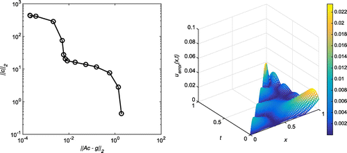
Figure 29. Case (b) of Example 3: The first plot shows the reconstructed Dirichlet data at $x=1$ for $\mathit{\delta }=5\%$, $h=2.2$, $\mathcal{N}=12$ and $\mathit{\lambda }={10}^{-7}$. The second plot shows the reconstructed Neumann data at $x=1$ for $\mathit{\delta }=5\%$, $h=2.2$, $\mathcal{N}=12$ and $\mathit{\lambda }={10}^{-7}$.

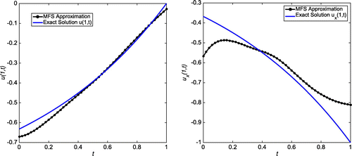
Case (c): Tol = 0.1, $\mathit{\delta }$ = 1%

In this case, our algorithm predicts the output as $h_{opt}=1.8$ with ${\mathcal{N}}_{opt}=8$. The left-hand plot of Figure 30 shows the L-curve for 1% of random noise, where source points have been placed with $h=1.8$, $\mathcal{N}=8$. The second plot shows the absolute error for all $(x,t)\in {\mathrm{\Omega }}_T$ for the noise level $\mathit{\delta }=1\%$ at $h=1.8$, $\mathcal{N}=8$ and with $\mathit{\lambda }={10}^{-5}$, which corresponds to the corner of the L-curve. The MFS approximations for u(1, t) and $u_x(1,t)$ are plotted for 1% noise level in Figure 31.

Figure 30. Case (c) of Example 3: The first plot shows the L-curve for $\mathit{\delta }=1\%$, $h=1.8$ and $\mathcal{N}=8$. The second plot shows the absolute error on the entire domain for $\mathit{\delta }=1\%$, $h=1.8$, $\mathcal{N}=8$ and $\mathit{\lambda }={10}^{-5}$. The corresponding RMSE over the entire domain is 0.0152709.

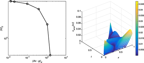
Figure 31. Case (c) of Example 3: The first plot shows the reconstructed Dirichlet data at $x=1$ for $\mathit{\delta }=1\%$, $h=1.8$, $\mathcal{N}=8$ and $\mathit{\lambda }={10}^{-5}$. The second plot shows the reconstructed Neumann data at $x=1$ for $\mathit{\delta }=1\%$, $h=1.8$, $\mathcal{N}=8$ and $\mathit{\lambda }={10}^{-5}$.

Case (d): Tol = 0.01, $\mathit{\delta }$ = 1%

Successive application of our algorithm yields the output as $h_{opt}=2.2$ with ${\mathcal{N}}_{opt}=12$ and $h_{opt}=2.4$ with ${\mathcal{N}}_{opt}=16$. In Figure 32, the first plot shows the L-curve for 1% of random noise at $h=2.2$ with $\mathcal{N}=12$, whereas the absolute error for all $(x,t)\in {\mathrm{\Omega }}_T$ for the noise level $\mathit{\delta }=1\%$ at $h=2.2$, $\mathcal{N}=12$ and with $\mathit{\lambda }={10}^{-6}$, which corresponds to the corner of the L-curve, is shown in the second plot. Similar plots have been shown in Figure 34 for $h=2.4$, $\mathcal{N}=16$ and $\mathit{\lambda }={10}^{-10}$. The MFS approximations for u(1, t) and $u_x(1,t)$ for $\mathit{\delta }=1\%$, $\mathcal{N}=12$, $\mathit{\lambda }={10}^{-6}$ at $h=2.2$ are plotted in Figure 33 and corresponding approximations for $\mathit{\delta }=1\%$, $\mathcal{N}=16$, $\mathit{\lambda }={10}^{-10}$ at $h=2.4$ are plotted in Figure 35.

Figure 32. Case (d) of Example 3: The first plot shows the L-curve for $\mathit{\delta }=1\%$, $h=2.2$ and $\mathcal{N}=12$. The second plot shows the absolute error on the entire domain for $\mathit{\delta }=1\%$, $h=2.2$, $\mathcal{N}=12$ and $\mathit{\lambda }={10}^{-6}$. The corresponding RMSE over the entire domain is 0.00291205.

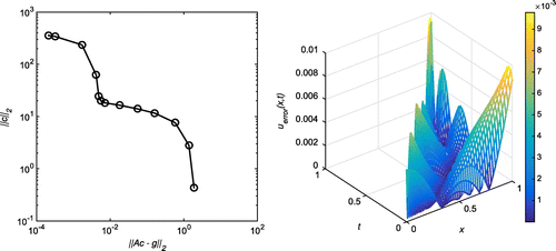
Figure 33. Case (d) of Example 3: The first plot shows the reconstructed Dirichlet data at $x=1$ for $\mathit{\delta }=1\%$, $h=2.2$, $\mathcal{N}=12$ and $\mathit{\lambda }={10}^{-6}$. The second plot shows the reconstructed Neumann data at $x=1$ for $\mathit{\delta }=1\%$, $h=2.2$, $\mathcal{N}=12$ and $\mathit{\lambda }={10}^{-6}$.

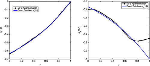
Figure 34. Case (d) of Example 3: The first plot shows the L-curve for $\mathit{\delta }=1\%$, $h=2.4$ and $\mathcal{N}=16$. The second plot shows the absolute error on the entire domain for $\mathit{\delta }=1\%$, $h=2.4$, $\mathcal{N}=16$ and $\mathit{\lambda }={10}^{-10}$. The corresponding RMSE over the entire domain is 0.000972025.

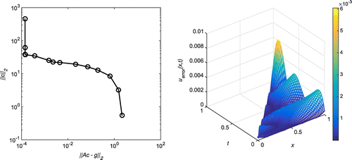
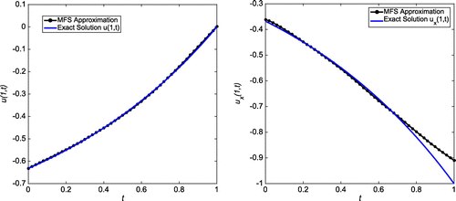
Figure 35. Case (d) of Example 3:The first plot shows the reconstructed Dirichlet data at $x=1$ for $\mathit{\delta }=1\%$, $h=2.4$, $\mathcal{N}=16$ and $\mathit{\lambda }={10}^{-10}$. The second plot shows the reconstructed Neumann data at $x=1$ for $\mathit{\delta }=1\%$, $h=2.4$, $\mathcal{N}=16$ and $\mathit{\lambda }={10}^{-10}$.

Observations

In cases (a), (b) and (c), we are concerned with $O({10}^{-2})$ accuracy for $\mathit{\delta }=5\%,1\%$, respectively. We observe that the MFS approximation for u(0, t) match well with the exact solution in all the cases. However, we note that it is difficult to obtain a good accuracy for $u_x(0,t)$ in the cases (a), (b), (c), especially as time t increases. However, reducing the Tol value in our algorithm in case (d) ($\mathit{\delta }=1\%$) leads to significantly improved results. One can get $O({10}^{-3})$ results, as seen in Figures 32 and 34, even when applying an error of $O({10}^{-2})$ on the Neumann boundary condition for $\mathit{\delta }=1\%$. A comparatively small number of collocation and source points, 12 and 16 respecively, were used to obtain such results. In this example also, one almost cannot distinguish the MFS approximations for u(0, t) and the exact solution, as seen in the left-hand plots of Figures 33 and 35. Increased numbers of source and collocation points in case (d) lead to a better MFS approximation of $u_x(0,t)$, as seen in the second plot of Figure 35).

Table 1. Quantitative information about running time of the algorithm.

Examples	Cases($Tol,\mathit{\delta }$)	$h_{opt}$	${\mathcal{N}}_{min}$	Time taken (s)
Example 1	a ($Tol=0.1,\mathit{\delta }=5\%$)	2.4/2.5	8	122
	b ($Tol=0.04,\mathit{\delta }=5\%$)	2.9	12	189
	c ($Tol=0.1,\mathit{\delta }=1\%$)	1.6	8	129
	d ($Tol=0.01,\mathit{\delta }=1\%$)	2.7	16	324
	d ($Tol=0.01,\mathit{\delta }=1\%$)	3.1	20	374
Example 2	a ($Tol=0.1,\mathit{\delta }=5\%$)	2.3/2.4	8	122
	b ($Tol=0.05,\mathit{\delta }=5\%$)	2.3	12	168
	c ($Tol=0.1,\mathit{\delta }=1\%$)	1.8	8	121
	d ($Tol=0.01,\mathit{\delta }=1\%$)	2.2	20	372
Example 3	a ($Tol=0.1,\mathit{\delta }=5\%$)	1.7/1.8	8	123
	b ($Tol=0.04,\mathit{\delta }=5\%$)	2.2	12	200
	c ($Tol=0.1,\mathit{\delta }=1\%$)	1.8	8	122
	d ($Tol=0.01,\mathit{\delta }=1\%$)	2.2	12	200
	d ($Tol=0.01,\mathit{\delta }=1\%$)	2.4	16	258

4.4. Closing remarks

Remark 1 (Testing better pseudo-boundaries):

The algorithm can be used for testing better pseudo-boundaries on which to place source points. For a given $\mathit{\delta }$, if one can obtain results of the same accuracy with fewer source (=collocation) points with a different pseudo-boundary, then it indicates that the new pseudo-boundary is better than the one we have used in this article. For example, if one can get $O({10}^{-2})$ accuracy or $Tol=0.1$ (see Cases (a) and (c) for each of the examples) with $\mathcal{N}=4$ for a fixed $\mathit{\delta }$(1% or 5%) with a different placement of source points, then, the new placement of source points can be considered better than the one considered in this article.

Remark 2 (Convergence property of MFS):

[Convergence property of MFS]The algorithm works on the principle that accuracy can be compensated for by increasing the number of source and collocation points. This fact can be seen by noting that if we reduce the tolerance level (demanding more accuracy), we need either the same or more source and collocation points (compare Cases (a) and (b) or Cases (c) and (d) of any example) to achieve the accuracy. Thus, the algorithm follows the convergence behaviour of the MFS. Moreover, we observed that, on decreasing $\mathit{\delta }$, we are able to recover more accuracy on the numerical solution.

Remark 3 (CAUTION):

[CAUTION]The value of $\mathit{\lambda }$ for which we attain $e_{max,opt}^{\mathit{\delta }}$ in the algorithm may not give the optimal regularization parameter. This fact was observed when we repeated our algorithm several times to determine the range of values of $h_{opt}$ for a fixed $\mathit{\delta }$ and fixed Tol. For a fixed relative % of $\mathit{\delta }$ (1 or 5%) and a fixed Tol, the value of $\mathit{\lambda }$ was different even when ${\mathcal{N}}_{opt}$ and $h_{opt}$ were the same. This is due to the fact that $\mathit{\lambda }$ not only depends on relative % of $\mathit{\delta }$, but a quantity, say $\mathrm{\Delta }(\mathit{\delta })$, where $\mathrm{\Delta }(\mathit{\delta })=N(0,{\mathit{\sigma }}^2)$ and $\mathit{\sigma }=\mathit{\delta }\times {max}_{(s(t),t),t\in (0,1]}|u_x(s(t),t)|$. Since the noise is random, $\mathit{\lambda }$ will depend on the random set of data which will vary every time we run our algorithm. However, it gives a rough idea of the regularization parameter. Confirmation of the regularization parameter can be done by the study of L-curve criteria once our algorithm produces the values $h_{opt}$, ${\mathcal{N}}_{opt}$ and using these values for the test purpose with a specific set of random data. On the other hand, existence of $h_{opt}$ and ${\mathcal{N}}_{opt}$ for which we attain $e_{max,opt}^{\mathit{\delta }}$ implies that there exists at least one set of random noise, and hence similar order of random noises, for which we are certain to get good accurate results. Furthermore, we want to comment that one can avoid an infinite loop that may arise in the algorithm if one demands a small Tol value. To avoid such cases, it is advisable to restrict the value of $\mathcal{N}$ by imposing an upper bound on it, say $\mathcal{N}=1000$. When $\mathcal{N}$ reaches 1000, one can impose a warning message. This upper bound on $\mathcal{N}$ is a reasonable choice, as it is out of scope of this article to solve a $1000\times 1000$ system to achieve the desired accuracy.

Remark 4 (Computational time of the algorithm):

[Computational time of the algorithm]The running time of our algorithm, which is given in Table 1 depends on many factors namely, $h_{min}$, $h_{max}$, $h_{step}$, ${\mathit{\lambda }}_{min}$, ${\mathit{\lambda }}_{max}$ and ${\mathit{\lambda }}_{step}$. We took $h_{min}=1$, $h_{max}=3.5$, $h_{step}=0.1$, ${\mathit{\lambda }}_{min}={10}^{-16}$, ${\mathit{\lambda }}_{max}={10}^{-1}$ and ${\mathit{\lambda }}_{step}={10}^1$. Nevertheless, the range of values of $\mathit{\lambda }$ is quite standard, the range of h can affect the running time of the algorithm. For larger values of tolerance ($Tol=0.1$, still consistent with the O(random noise)), we observed that there a bigger interval for h (see case (a) $h_{opt}=2.4,2.5$ for Example 1, $h_{opt}=2.3,2.4$ for Example 2 and $h_{opt}=1.7,1.8$ for Example 3. In fact, in Case (c) for each of the examples, we got narrower range of values of $h_{opt}$, which are excluded from this article) for which we can get good consistent results. In such cases, one can increase $h_{step}$ say to $h_{step}=0.2$ without changing $h_{min}$ and $h_{max}$. Thus, one needs to solve a smaller system of equations, so that the process of finding the optimal h is faster and thus, more computationally efficient. Moreover, from the experiments, we observe that for all the examples the optimal location of source points lies between 1.6 to 3.1 so that one can change the range of h, say $h_{min}=1.6$ and $h_{max}=3.1$, which will affect the running time of our algorithm. Similarly, one can change these parameters for each of the examples so that the running time of the algorithm will vary for each of the examples. On the other hand, one can fix the source points and allow the number of collocation points to vary, or vice versa, in the algorithm. However, it will affect computational time of the algorithm blockwise.

Remark 5 (An important observation):

For a fixed $\mathit{\delta }$, the authors in [9] tried to increase the number of source and collocation points to get a more accurate numerical solution, keeping h fixed. They found that it does not increase significantly the accuracy of the numerical results. Precisely, the implicit assumption of increasing the number of source and collocation points is that the accuracy depends on this number. On the contrary, our algorithm predicts that for a fixed $\mathit{\delta }$, the accuracy depends both on the location h and the number of source and collocation points ($\mathcal{N}$). To be precise, we observed that the accuracy cannot be increased for these kind of problems simply by increasing the number of source and collocation points for an a priori fixed h.

Remark 6 (Physical discussion):

Examples 1 and 2 can be thought of as situations where molten material that is cooled at $x=0$ solidifies. Based on knowledge of the material’s melting temperature and the evolution of the solid/liquid interface, the temperature and the heat flux at $x=0$ have been reconstructed. In these examples, the extent of the region in which the problem is being solved increases with time; Examples 1 and 2 differ in that the interface moves linearly with time in Example 1, but non-linearly in Example 2. On the other hand, in the ablation-related Example 3, the extent of the region is decreasing with time. In this case, a solid occupies the region $0\le x\le 1,$ and the material begins to ablate from $x=0;$ based on knowledge of the material’s melting temperature and the evolution of the ablation interface, the temperature and the heat flux at $x=1$ have been reconstructed. In view of the large set of results, it is not possible to discuss each one in detail, but we can observe several trends. It is generally much easier to reconstruct the temperature than the heat flux, as was already observed in [9]; moreover, it is easier to do this with more accurate knowledge about the material’s melting temperature and the location of the phase-change interface, i.e. when $\mathit{\delta }$ is smaller. These conclusions do not seem to be affected by whether the extent of the solution domain increases or decreases with time.

5. Conclusion and future work

In this article, we proposed a simple, practical and efficient algorithm which determines the optimal location of the source points, along with the minimum number of source and collocation points required to generate desired accuracy, in the application of the MFS for the inverse Stefan problems, given the relative amount of noise added to the boundary conditions. The effectiveness of the algorithm is checked for several benchmark problems where it yields good, accurate results. Surprisingly, even with $O({10}^{-2})$ noise for $\mathit{\delta }=1\%$, our algorithm is able to find $h_{opt}$ with just a few source points (see Case (d) for each of the examples) for which the absolute maximum error is of $O({10}^{-3})$. However, this was not the case with $\mathit{\delta }=5\%$. We got $O({10}^{-2})$ results for $\mathit{\delta }=5\%$ which is consistent with the noise applied on the boundary. On the other hand, a quantitative understanding of the algorithm would justify the cost of computation since, at each iteration, one needs to solve systems with only smaller values of $\mathcal{N}$.

This algorithm was shown to work for the inverse Stefan problem, but we believe that it, or a perturbed version, will work for other classes of problems, such as direct problems or inverse Cauchy–Stefan problems. In this article, we observed that our algorithm reconstructs the Dirichlet data well; however, the reconstruction of the Neumann data still has some issues, at least in some cases, and needs further attention. We will consider this issue in future work. Moreover, we will show the effectiveness of such an algorithm for inverse Cauchy–Stefan problems. Further future work consists of showing a modified algorithm for inverse and Cauchy–Stefan problems when the location of the interface is unknown.

Acknowledgements

The authors wish to thank the referees for the valuable suggestions.

Additional information

Funding

The first author would like to thank the financial support received from the FAPESP [grant number 2016/19648-9]. The second author acknowledges the award of a visiting researcher grant from the University of São Paulo.

Notes

No potential conflict of interest was reported by the authors.

References

- Rubinstein LI . The Stefan problem. Providence (RI): American Mathematical Society; 1971. Translated from the Russian by Solomon AD.Translations of Mathematical Monographs, Vol. 27.
- Gol’dman NL . Inverse Stefan problems. Vol. 412, Mathematics and its applications. Dordrecht: Kluwer Academic Publishers Group; 1997.
- Słota D . Identification of the cooling condition in 2D and 3D continuous casting processes. Num Heat Trans B. 2009;55:155–176.
- Słota D . Reconstruction of the boundary condition in the problem of the binary alloy solidification. Arch Metall Mater. 2011;56:279–285.
- Wang Z , Yao M , Wang X , et al. Inverse problem-coupled heat transfer model for steel continuous casting. J Mater Proc Tech. 2014;214:44–49.
- O’Mahoney D , Browne DJ . Use of an experiment and an inverse method to study interface heat transfer during solidification in the investment casting process. Exp Thermal Fluid Sci. 2000;22:111–122.
- Okamoto K , Li BQ . A regularization method for the inverse design of solidification processes with natural convection. Int J Heat Mass Transfer. 2007;50:4409–4423.
- Chantasiriwan S , Johansson BT , Lesnic D . The method of fundamental solutions for free surface Stefan problems. Eng Anal Bound Elem. 2009;33(4):529–538.
- Johansson BT , Lesnic D , Reeve T . A method of fundamental solutions for the one-dimensional inverse Stefan problem. App Math Modell. 2011;35:4367–4378.
- Johansson BT , Lesnic D , Reeve T . The method of fundamental solutions for the two-dimensional inverse Stefan problem. Inverse Probl Sci Eng. 2014;22:112–129.
- Karageorghis A , Lesnic D , Marin L . A survey of applications of the MFS to inverse problems. Inverse Probl Sci Eng. 2011;19(3):309–336.
- Mathon R , Johnston RL . The approximate solution of elliptic boundary-value problems by fundamental solutions. SIAM J Numer Anal. 1977;14(4):638–650.
- Johnston RL , Fairweather G . The method of fundamental solutions for problems in potential flow. Appl Math Modell. 1984;8(4):265–270.
- Fairweather G , Karageorghis A . The method of fundamental solutions for elliptic boundary value problems. Adv Comput Math. 1998;9(1–2):69–95.
- Gorzelaczyk P , Koodziej JA . Some remarks concerning the shape of the source contour with application of the method of fundamental solutions to elastic torsion of prismatic rods. Eng Anal Boundary Elem. 2008;32(1):64–75.
- Alves CJS . On the choice of source points in the method of fundamental solutions. Eng Anal Bound Elem. 2009;33(12):1348–1361.
- Cisilino AP , Sensale B . Application of a simulated annealing algorithm in the optimal placement of the source points in the method of the fundamental solutions. Comput Mech. 2002;28(2):129–136.
- Karageorghis A . A practical algorithm for determining the optimal pseudo-boundary in the method of fundamental solutions. Adv Appl Math Mech. 2009;1(4):510–528.
- Wong KY , Ling L . Optimality of the method of fundamental solutions. Eng Anal Bound Elem. 2011;35(1):42–46.
- Chen CS , Karageorghis A , Li Y . On choosing the location of the sources in the MFS. Numer Algorithms. 2016;72(1):107–130.
- Cannon JR , Douglas J Jr . The Cauchy problem for the heat equation. SIAM J Numer Anal. 1967;4:317–336.
- Cannon JR , Primicerio M . Remarks on the one-phase Stefan problem for the heat equation with the flux prescribed on the fixed boundary. J Math Anal Appl. 1971;35(2):361–373.
- Cannon JR , Hill CD . Existence, uniqueness, stability, and monotone dependence in a Stefan problem for the heat equation. J Math Mech. 1967;17(17):1–19.
- Chen CS , Cho HA , Golberg MA . Some comments on the ill-conditioning of the method of fundamental solutions. Eng Anal Boundary Element. 2006;30(5):405–410.
- Ramachandran PA . Method of fundamental solutions: singular value decomposition analysis. Commun Numer Methods Eng. 2002;18(11):789–801.
- Ang DD , Dinh APN , Thanh DN . An inverse Stefan problem: identification of boundary value. J Comput Appl Math. 1996;66(1):75–84.
- Andrews JG , Atthey DR . On the motion of an intensely heated evaporating boundary. J Inst Math Appl. 1975;15:59–72.
- Chen Y-K , Milos FS . Ablation and thermal response program for spacecraft heatshield analysis. J Spacecraft Rockets. 1999;36(3):475–483.
- Campbell AJ , Humayun M . Trace element microanalysis in iron meteorites by laser ablation ICPMS. Anal Chem. 1999;71(5):939–946.
- Lin W-S . Steady ablation on the surface of a two-layer composite. Int J Heat Mass Trans. 2005;48(25–26):5504–5519.
- Tayler AB . Mathematical models in applied mechanics. Oxford: Oxford University Press; 2001.
- Johnson WD . The profile of maturity in alpine glacial erosion. J Geology. 1904;12(7):569–578.
- Namenanee K , McKenzie J , Kosa E , et al . A new approach for catheter ablation of atrial fibrillation: mapping of the electrophysiologic substrate. J Amer College Cardiol. 2004;43(11):2044–2053.