Application of the cut-off projection to solve a backward heat conduction problem in a two-slab composite system

ABSTRACT

The main goal of this paper is applying the cut-off projection for solving one-dimensional backward heat conduction problem in a two-slab system with a perfect contact. In a constructive manner, we commence by demonstrating the Fourier-based solution that contains the drastic growth due to the high-frequency nature of the Fourier series. Such instability leads to the need of studying the projection method where the cut-off approach is derived consistently. In the theoretical framework, the first two objectives are to construct the regularized problem and prove its stability for each noise level. Our second interest is estimating the error in $L^2$-norm. Another supplementary objective is computing the eigen-elements. All in all, this paper can be considered as a preliminary attempt to solve the heating/cooling of a two-slab composite system backward in time. Several numerical tests are provided to corroborate the qualitative analysis.

KEYWORDS:

• Two-slab system
• cut-off projection
• backward heat conduction problem
• ill-posedness
• regularized solution
• error estimates

AMS SUBJECT CLASSIFICATIONS:

• 35K05
• 42A20
• 47A52
• 65J20

1. Introduction

The backward-in-time heat conduction problem has been scrutinized for a long time by many approaches with fast-adapting and effectively distinct strategies. This problem plays a critical role in different fields of study, for example, enabling us to determine the initial temperature of a volcano when the eruption has already started, or recover noisy, blurry digital images acquired by camera sensors.

The need for finding numerical solutions of various kinds of such equations is originated from its natural instability due to the drastic growth of the solutions. Once inaccurate final data are applied to the partial differential equation (PDE), one could obtain a totally wrong solution even if the final data are measured as accurately as possible. In fact, the measured data in real-life applications are always inaccurate. Thus, studies on regularization methods have attracted a considerable amount of attention, where stable approximate solutions were developed year by year. Several comprehensive materials are given in the textbook of Lattès and Lions [1], and papers such as [2–11].

In this paper, we consider the heat transfer problem in a two slabs composite $(-b<x<0)$ and $\left(0<x<a\right)$. We also follow the notations in [12]. In particular, the problem, in which the time interval is defined by $J:=\left[t_0,t_f\right]$ for $t_0\ge 0,t_f>0$, can be expressed as:(1) $$\begin{array}{cc}\hfill {\rho }_b{c}_b\frac{\partial T_b}{\partial t}& =K_b\frac{{\partial }^2{T}_b}{\partial x^2},-b<x<0,t\in J,\hfill \end{array}$$(1) (2) $$\begin{array}{cc}\hfill {\rho }_a{c}_a\frac{\partial T_a}{\partial t}& =K_a\frac{{\partial }^2{T}_a}{\partial x^2},0<x<a,t\in J.\hfill \end{array}$$(2)

The boundary conditions are:(3) $$\begin{array}{cc}\hfill \frac{\partial T_b}{\partial x}& =0\text{at}x=-b,\frac{\partial T_a}{\partial x}=0\text{at}x=a,t\in J\hfill \end{array}$$(3) (4) $$\begin{array}{cc}\hfill T_b& =T_a,K_b\frac{\partial T_b}{\partial x}=K_a\frac{\partial T_a}{\partial x}\text{at}x=0,t\in J.\hfill \end{array}$$(4)

The model (1(1) $$\begin{array}{cc}\hfill {\rho }_b{c}_b\frac{\partial T_b}{\partial t}& =K_b\frac{{\partial }^2{T}_b}{\partial x^2},-b<x<0,t\in J,\hfill \end{array}$$(1) )–(4(4) $$\begin{array}{cc}\hfill T_b& =T_a,K_b\frac{\partial T_b}{\partial x}=K_a\frac{\partial T_a}{\partial x}\text{at}x=0,t\in J.\hfill \end{array}$$(4) ) involves a number of dimensionless quantities, namely the temperature $T_{\alpha }$ (${}^{\circ }\text{C}$), mass density ${\rho }_{\alpha }$ (g/${\text{cm}}^3$), specific heat $c_{\alpha }$ (cal/$(\text{g}{·}^{\circ }\text{C})$), and thermal conductivity $K_{\alpha }$ (cal/$(\text{cm}·\text{sec}{·}^{\circ }\text{C})$). Here the index $\alpha$ indicates either material a or b, i.e. $\alpha \in \{a,b\}$. The perfect contact in (4(4) $$\begin{array}{cc}\hfill T_b& =T_a,K_b\frac{\partial T_b}{\partial x}=K_a\frac{\partial T_a}{\partial x}\text{at}x=0,t\in J.\hfill \end{array}$$(4) ) indicates that the temperature and heat flux are continuous at the interface.

The model (1(1) $$\begin{array}{cc}\hfill {\rho }_b{c}_b\frac{\partial T_b}{\partial t}& =K_b\frac{{\partial }^2{T}_b}{\partial x^2},-b<x<0,t\in J,\hfill \end{array}$$(1) )–(4(4) $$\begin{array}{cc}\hfill T_b& =T_a,K_b\frac{\partial T_b}{\partial x}=K_a\frac{\partial T_a}{\partial x}\text{at}x=0,t\in J.\hfill \end{array}$$(4) ) is supplemented with the terminal measured data $T_{\alpha }^{\epsilon }\left(x,t_f\right)$ which satisfy:(5) $$\begin{array}{c}\hfill {∥T_a\left(·,t_f\right)-T_a^{\epsilon }\left(·,t_f\right)∥}_{L^2\left(0,a\right)}+{∥T_b\left(·,t_f\right)-T_b^{\epsilon }\left(·,t_f\right)∥}_{L^2\left(-b,0\right)}\le \epsilon ,\end{array}$$(5)

where $0<\epsilon \ll 1$ represents the maximum bound of errors arising in measurement. Henceforward, our task is to identify the initial value $T_{\alpha }^{\epsilon }\left(x,t_0\right),-b\le x\le a$.

Our main objective is to prove the ill-posedness of the aforementioned model and then deal with it by using the cut-off projection method. Historically, there have been several works that treat ill-posed problems using this method. For instances, Daripa and his co-workers in [13,14] contributed significantly. In particular, the cut-off method [13] was used to control the spurious effects on the solution due to short wave components of the round-off and truncation errors. Recently, the cut-off method was utilized by Regińska and Regiński [15] and Tuan et al. [16] to stabilize the $cosh\left(x\right)$- and $sinh\left(x\right)/x$-like growth in a Cauchy problem for the 3D Helmholtz equation.

This paper is fivefold. Section 2 is devoted to the eigen-elements and ill-posedness of the model. We compute the approximate eigenvalues and eigenfunctions, along with providing the temperature solution by Fourier-based modes. In Section 3, the cut-off method is described by providing the regularized problem corresponding to the terminal measured data $T_{\alpha }^{\epsilon }\left(x,t_f\right)$. We also show the error estimates which clearly imply the stability of the regularized solution at each noise level. Lastly, some numerical tests are given in Section 4, whilst Section 5 is dedicated to a few conclusions and pointing out problems for possible further development.

2. Eigen-elements

In the context of Fourier representations, the eigen-elements including the eigenvalues and eigenfunctions can be obtained by solving the Sturm–Liouville problem. Such problem would be of the form:(6) $$\begin{array}{c}\hfill {\varphi }_{\alpha }^{″}+{\lambda }_{\alpha }^2{\varphi }_{\alpha }=0\text{for}\alpha \in \left\{a,b\right\},\end{array}$$(6)

associated with the boundary conditions (3(3) $$\begin{array}{cc}\hfill \frac{\partial T_b}{\partial x}& =0\text{at}x=-b,\frac{\partial T_a}{\partial x}=0\text{at}x=a,t\in J\hfill \end{array}$$(3) ) and (4(4) $$\begin{array}{cc}\hfill T_b& =T_a,K_b\frac{\partial T_b}{\partial x}=K_a\frac{\partial T_a}{\partial x}\text{at}x=0,t\in J.\hfill \end{array}$$(4) ). After some straightforward calculations and using (3(3) $$\begin{array}{cc}\hfill \frac{\partial T_b}{\partial x}& =0\text{at}x=-b,\frac{\partial T_a}{\partial x}=0\text{at}x=a,t\in J\hfill \end{array}$$(3) ) one has(7) $$\begin{array}{c}\hfill {\varphi }_b(x)={\theta }_{b}cos\left({\lambda }_b\left(x+b\right)\right),{\varphi }_a(x)={\theta }_{a}cos\left({\lambda }_a\left(x-a\right)\right),\end{array}$$(7)

where ${\theta }_a,{\theta }_b$ are constants.

Applying the transmission conditions (4(4) $$\begin{array}{cc}\hfill T_b& =T_a,K_b\frac{\partial T_b}{\partial x}=K_a\frac{\partial T_a}{\partial x}\text{at}x=0,t\in J.\hfill \end{array}$$(4) ) at the interface $x=0$, we arrive at(8) $$\begin{array}{cc}& {\theta }_{b}cos\left({\lambda }_{b}b\right)-{\theta }_{a}cos\left({\lambda }_{a}a\right)=0,\hfill \end{array}$$(8) (9) $$\begin{array}{cc}& {\theta }_b{K}_b{\lambda }_{b}sin\left({\lambda }_{b}b\right)+{\theta }_a{K}_a{\lambda }_{a}sin\left({\lambda }_{a}a\right)=0,\hfill \end{array}$$(9)

which lead to the transcendental equation for eigenvalues:(10) $$\begin{array}{c}\hfill K_b{\lambda }_{b}sin\left({\lambda }_{b}b\right)cos\left({\lambda }_{a}a\right)+K_a{\lambda }_{a}sin\left({\lambda }_{a}a\right)cos\left({\lambda }_{b}b\right)=0.\end{array}$$(10)

For brevity, we denote the thermal diffusivities (${\text{cm}}^2/\text{sec}$) by$${\kappa }_{\alpha }=\frac{K_{\alpha }}{{\rho }_{\alpha }{c}_{\alpha }}\text{for}\alpha \in \left\{a,b\right\}.$$

Since we need the same time dependence in both slabs, the condition(11) $$\begin{array}{c}\hfill {\kappa }_b{\lambda }_b^2={\kappa }_a{\lambda }_a^2\end{array}$$(11)

is required. Hereby, the above equation enables us to derive the new eigenvalue condition from (10(10) $$\begin{array}{c}\hfill K_b{\lambda }_{b}sin\left({\lambda }_{b}b\right)cos\left({\lambda }_{a}a\right)+K_a{\lambda }_{a}sin\left({\lambda }_{a}a\right)cos\left({\lambda }_{b}b\right)=0.\end{array}$$(10) ):(12) $$\begin{array}{c}\hfill \frac{K_b}{\sqrt{{\kappa }_b}}sin\left({\lambda }_{b}b\right)cos\left({\lambda }_{a}a\right)+\frac{K_a}{\sqrt{{\kappa }_a}}sin\left({\lambda }_{a}a\right)cos\left({\lambda }_{b}b\right)=0.\end{array}$$(12)

To sum up, the two transcendental Equations (11(11) $$\begin{array}{c}\hfill {\kappa }_b{\lambda }_b^2={\kappa }_a{\lambda }_a^2\end{array}$$(11) ) and (12(12) $$\begin{array}{c}\hfill \frac{K_b}{\sqrt{{\kappa }_b}}sin\left({\lambda }_{b}b\right)cos\left({\lambda }_{a}a\right)+\frac{K_a}{\sqrt{{\kappa }_a}}sin\left({\lambda }_{a}a\right)cos\left({\lambda }_{b}b\right)=0.\end{array}$$(12) ) allow us to compute the eigenvalues ${\lambda }_{\mathit{an}},{\lambda }_{\mathit{bn}}$ for $n\in \mathbb{N}$.

2.1. A computational approach

The Equations (11(11) $$\begin{array}{c}\hfill {\kappa }_b{\lambda }_b^2={\kappa }_a{\lambda }_a^2\end{array}$$(11) ) and (12(12) $$\begin{array}{c}\hfill \frac{K_b}{\sqrt{{\kappa }_b}}sin\left({\lambda }_{b}b\right)cos\left({\lambda }_{a}a\right)+\frac{K_a}{\sqrt{{\kappa }_a}}sin\left({\lambda }_{a}a\right)cos\left({\lambda }_{b}b\right)=0.\end{array}$$(12) ) spontaneously generate a system of nonlinear algebraic equations with 2N variables ${\lambda }_{\mathit{bn}}$ and ${\lambda }_{\mathit{an}}$ for $n\in \left\{0,...,N\right\}$. From the numerical point of view, the common way is to use the Newton method which is known as the one-step iterative scheme with quadratic convergence [17] for solving equations of the form $\text{F}\left(\text{x}\right)=0$. Besides, so far there have been several effective approaches such as the Newton-Simpson’s method of [18] and the improved Newton’s method by the Closed-Open quadrature formula of [19]. However, there would be some basic impediments if we exploit such approaches. Noticeably, the transcendental system (11(11) $$\begin{array}{c}\hfill {\kappa }_b{\lambda }_b^2={\kappa }_a{\lambda }_a^2\end{array}$$(11) ) and (12(12) $$\begin{array}{c}\hfill \frac{K_b}{\sqrt{{\kappa }_b}}sin\left({\lambda }_{b}b\right)cos\left({\lambda }_{a}a\right)+\frac{K_a}{\sqrt{{\kappa }_a}}sin\left({\lambda }_{a}a\right)cos\left({\lambda }_{b}b\right)=0.\end{array}$$(12) ) has infinitely many roots and furthermore, we cannot ensure that the obtained solutions correspond one-to-one to the indexes n, which means that the result may be missed out or exceeded. Thus, by varying initial guesses ${\text{x}}_0$, it would produce a few confusing results. For instance, taking $K_{\alpha }={\kappa }_{\alpha }=1$, we easily obtain the family of solutions(13) $$\begin{array}{c}\hfill {\lambda }_{\alpha k}=\frac{k\pi }{a+b}\text{for}k\in \mathbb{N},\end{array}$$(13)

then with $a=3,b=5$ and the two initial points$${\text{x}}_0:={\left[\begin{array}{ccccc}0& 1& \cdots & N-1& N\\ 0& 1& \cdots & N-1& N\end{array}\right]}^{\text{T}}\text{and}{\text{x}}_1:=0.5{\text{x}}_0,$$

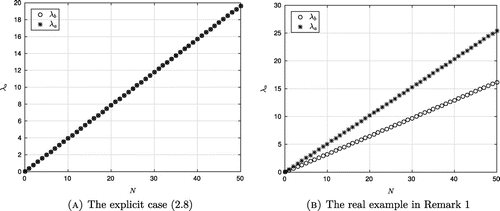
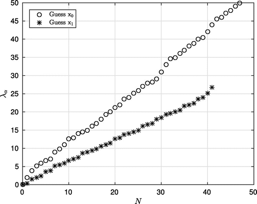
the eigenvalues governed by the standard Newton method (for $N=50$) are showed in Figure 1 for comparison. It is apparent that there are many differences between the two figures. Basically, the actual final eigenvalue with $N=50$ is approximately 19.63495 from (13(13) $$\begin{array}{c}\hfill {\lambda }_{\alpha k}=\frac{k\pi }{a+b}\text{for}k\in \mathbb{N},\end{array}$$(13) ), while the others are, respectively, 49.87278 and 26.70353 in Figure 1. The results also indicate that with the guess ${\text{x}}_0$ there are 48 admissible values obtained by the elimination of equal values whilst there are only 42 values for the guess ${\text{x}}_1$.

Figure 1. Numerical eigenvalues for the explicit case (13(13) $$\begin{array}{c}\hfill {\lambda }_{\alpha k}=\frac{k\pi }{a+b}\text{for}k\in \mathbb{N},\end{array}$$(13) ) using the standard Newton method with different initial guesses ${\text{x}}_0$ and ${\text{x}}_1$ at the 10th iteration and with the stopping constant $\delta ={10}^{-10}$.

In order to overcome this issue, we apply the built-in function fzero of MATLAB to several different initial points over some pre-defined range. Thanks to the structure of the transcendental Equations (11(11) $$\begin{array}{c}\hfill {\kappa }_b{\lambda }_b^2={\kappa }_a{\lambda }_a^2\end{array}$$(11) ) and (12(12) $$\begin{array}{c}\hfill \frac{K_b}{\sqrt{{\kappa }_b}}sin\left({\lambda }_{b}b\right)cos\left({\lambda }_{a}a\right)+\frac{K_a}{\sqrt{{\kappa }_a}}sin\left({\lambda }_{a}a\right)cos\left({\lambda }_{b}b\right)=0.\end{array}$$(12) ), we are capable of reducing the system to the following equation:(14) $$\begin{array}{c}\hfill \frac{K_b}{\sqrt{{\kappa }_b}}sin\left({\lambda }_{b}b\right)cos\left(\sqrt{\frac{{\kappa }_b}{{\kappa }_a}}{\lambda }_{b}a\right)+\frac{K_a}{\sqrt{{\kappa }_a}}sin\left(\sqrt{\frac{{\kappa }_b}{{\kappa }_a}}{\lambda }_{b}a\right)cos\left({\lambda }_{b}b\right)=0,\end{array}$$(14)

where we have derived from (11(11) $$\begin{array}{c}\hfill {\kappa }_b{\lambda }_b^2={\kappa }_a{\lambda }_a^2\end{array}$$(11) ) that(15) $$\begin{array}{c}\hfill {\lambda }_a=\sqrt{\frac{{\kappa }_b}{{\kappa }_a}}{\lambda }_b\end{array}$$(15)

and substituted this to (12(12) $$\begin{array}{c}\hfill \frac{K_b}{\sqrt{{\kappa }_b}}sin\left({\lambda }_{b}b\right)cos\left({\lambda }_{a}a\right)+\frac{K_a}{\sqrt{{\kappa }_a}}sin\left({\lambda }_{a}a\right)cos\left({\lambda }_{b}b\right)=0.\end{array}$$(12) ). Once ${\lambda }_b$ is found, it is straightforward to compute the corresponding ${\lambda }_a$ from (15(15) $$\begin{array}{c}\hfill {\lambda }_a=\sqrt{\frac{{\kappa }_b}{{\kappa }_a}}{\lambda }_b\end{array}$$(15) ). The algorithm to compute the first N non-negative eigenvalues ${\lambda }_{\mathit{bn}}$ from (14(14) $$\begin{array}{c}\hfill \frac{K_b}{\sqrt{{\kappa }_b}}sin\left({\lambda }_{b}b\right)cos\left(\sqrt{\frac{{\kappa }_b}{{\kappa }_a}}{\lambda }_{b}a\right)+\frac{K_a}{\sqrt{{\kappa }_a}}sin\left(\sqrt{\frac{{\kappa }_b}{{\kappa }_a}}{\lambda }_{b}a\right)cos\left({\lambda }_{b}b\right)=0,\end{array}$$(14) ) is described as follows:

Figure 2. Numerical eigenvalues using the MATLAB-built-in function fzero.

Remark 1:

A complicated case is provided in Figure 2(b) where the eigenvalues cannot be solved explicitly. The materials we illustrate are the copper versus the molybdeum, which was experienced by Josell et al. [20], providing ${\kappa }_{\alpha }\in \left\{0.838,0.339\right\}$ and $K_{\alpha }\in \left\{3.42,1.05\right\}$, respectively. Here, this case is governed by the same parameters of the previous explicit case (13(13) $$\begin{array}{c}\hfill {\lambda }_{\alpha k}=\frac{k\pi }{a+b}\text{for}k\in \mathbb{N},\end{array}$$(13) ), i.e. $N=50,a=3,b=5$, with $d=10$ and $\delta ={10}^{-3}$. By comparing Figures 1 and 2, it is easy to see the differences and how well the simple algorithm works. Especially, the computed final numerical eigenvalue, i.e. ${\lambda }_{b50}=19.63495$ in Figure 2(a), is very closed to the exact value. The only disadvantage of this approach is the long execution time that may rise in higher dimensions.

Now, let us consider the eigenfunctions ${\varphi }_{\alpha }$. By choosing appropriate constants ${\theta }_a$ and ${\theta }_b$ in (7(7) $$\begin{array}{c}\hfill {\varphi }_b(x)={\theta }_{b}cos\left({\lambda }_b\left(x+b\right)\right),{\varphi }_a(x)={\theta }_{a}cos\left({\lambda }_a\left(x-a\right)\right),\end{array}$$(7) ), we obtain the following eigenfunctions:(16) $$\begin{array}{c}\hfill {\tilde{\varphi }}_n(x)={\varphi }_{\mathit{bn}}(x)=\frac{cos\left({\lambda }_{\mathit{bn}}\left(x+b\right)\right)}{cos\left({\lambda }_{\mathit{bn}}b\right)}\text{for the left slab}\left(-b<x<0\right),\end{array}$$(16)

and(17) $$\begin{array}{c}\hfill {\tilde{\varphi }}_n(x)={\varphi }_{\mathit{an}}(x)=\frac{cos\left({\lambda }_{\mathit{an}}\left(x-a\right)\right)}{cos\left({\lambda }_{\mathit{an}}a\right)}\text{for the right slab}\left(0<x<a\right).\end{array}$$(17)

Remark 2:

For different indexes $m\ne n$, the eigenfunctions ${\tilde{\varphi }}_m$ and ${\tilde{\varphi }}_n$ are orthogonal in the sense that(18) $$\begin{array}{c}\hfill \frac{K_b}{{\kappa }_b}{〈{\tilde{\varphi }}_m,{\tilde{\varphi }}_n〉}_{L^2\left(-b,0\right)}+\frac{K_a}{{\kappa }_a}{〈{\tilde{\varphi }}_m,{\tilde{\varphi }}_n〉}_{L^2\left(0,a\right)}=0.\end{array}$$(18)

On the other hand, we also obtain the same equality for the derivatives of such eigenfunctions. In fact, these functions are orthogonal in the sense that$$K_b{〈{\tilde{\varphi }}_m^{{}^{\prime }},{\tilde{\varphi }}_n^{{}^{\prime }}〉}_{L^2\left(-b,0\right)}+K_a{〈{\tilde{\varphi }}_m^{{}^{\prime }},{\tilde{\varphi }}_n^{{}^{\prime }}〉}_{L^2\left(0,a\right)}=0.$$

Let us denote$$\begin{array}{cc}\hfill {\mathcal{N}}_n& :=\frac{K_b}{{\kappa }_b}{∥{\tilde{\varphi }}_n∥}_{L^2\left(-b,0\right)}^2+\frac{K_a}{{\kappa }_a}{∥{\tilde{\varphi }}_n∥}_{L^2\left(0,a\right)}^2\hfill \\ \hfill & =\frac{b{K}_b}{2{\kappa }_b}\frac{1}{{cos}^2\left({\lambda }_{\mathit{bn}}b\right)}+\frac{a{K}_a}{2{\kappa }_a}\frac{1}{{cos}^2\left({\lambda }_{\mathit{an}}a\right)}\text{for}n\in {\mathbb{N}}^{\ast },\hfill \end{array}$$ $$\begin{array}{cc}\hfill {\mathcal{M}}_n& :=K_b{∥{\tilde{\varphi }}_n^{{}^{\prime }}∥}_{L^2\left(-b,0\right)}^2+K_a{∥{\tilde{\varphi }}_n^{{}^{\prime }}∥}_{L^2\left(0,a\right)}^2\hfill \\ \hfill & =\frac{b{K}_b}{2}\frac{{\lambda }_{\mathit{bn}}^2}{{cos}^2\left({\lambda }_{\mathit{bn}}b\right)}+\frac{a{K}_a}{2}\frac{{\lambda }_{\mathit{an}}^2}{{cos}^2\left({\lambda }_{\mathit{an}}a\right)}\text{for}n\in {\mathbb{N}}^{\ast },\hfill \end{array}$$

with$${\mathcal{N}}_0:=\frac{K_b}{{\kappa }_b}{∥{\tilde{\varphi }}_0∥}_{L^2\left(-b,0\right)}^2+\frac{K_a}{{\kappa }_a}{∥{\tilde{\varphi }}_0∥}_{L^2\left(0,a\right)}^2=\frac{b{K}_b}{{\kappa }_b}+\frac{a{K}_a}{{\kappa }_a},$$

and$${\mathcal{M}}_0:=K_b{∥{\tilde{\varphi }}_0^{{}^{\prime }}∥}_{L^2\left(-b,0\right)}^2+K_a{∥{\tilde{\varphi }}_0^{{}^{\prime }}∥}_{L^2\left(0,a\right)}^2=0.$$

3. Main results

3.1. Solution by Fourier-mode and Instability

From the transcendental Equations (11(11) $$\begin{array}{c}\hfill {\kappa }_b{\lambda }_b^2={\kappa }_a{\lambda }_a^2\end{array}$$(11) )–(12(12) $$\begin{array}{c}\hfill \frac{K_b}{\sqrt{{\kappa }_b}}sin\left({\lambda }_{b}b\right)cos\left({\lambda }_{a}a\right)+\frac{K_a}{\sqrt{{\kappa }_a}}sin\left({\lambda }_{a}a\right)cos\left({\lambda }_{b}b\right)=0.\end{array}$$(12) ) and the formulation of the eigenfunctions in (16(16) $$\begin{array}{c}\hfill {\tilde{\varphi }}_n(x)={\varphi }_{\mathit{bn}}(x)=\frac{cos\left({\lambda }_{\mathit{bn}}\left(x+b\right)\right)}{cos\left({\lambda }_{\mathit{bn}}b\right)}\text{for the left slab}\left(-b<x<0\right),\end{array}$$(16) )–(17(17) $$\begin{array}{c}\hfill {\tilde{\varphi }}_n(x)={\varphi }_{\mathit{an}}(x)=\frac{cos\left({\lambda }_{\mathit{an}}\left(x-a\right)\right)}{cos\left({\lambda }_{\mathit{an}}a\right)}\text{for the right slab}\left(0<x<a\right).\end{array}$$(17) ), we are competent to construct the temperature solution throughout the two-slab system, denoted by $T\left(x,t\right)$. Basically, the Fourier-mode for the solution of this system cannot be obtained in the same manner with the classical backward heat equation due to the non-trivial orthogonality (showed in Remark 2) in which we cannot make equivalent computations. Nevertheless, we are still able to compute it by following the structural property of the solution in the classical case.

By assigning ${\overline{\lambda }}_n:={\kappa }_b{\lambda }_{\mathit{bn}}^2={\kappa }_a{\lambda }_{\mathit{an}}^2$, the temperature solution (in the finite series truncated computational sense) would be of the following form:(19) $$\begin{array}{c}\hfill T_N\left(x,t\right)=\sum _{n=0}^N{C}_n{e}^{{\overline{\lambda }}_n\left(t_f-t\right)}{\tilde{\varphi }}_n\left(x\right),\left(x,t\right)\in \left[-b,a\right]\times \left[t_0,t_f\right],\end{array}$$(19)

for some $N\in \mathbb{N}$ and the data associated with the final state of temperature is provided by(20) $$\begin{array}{c}\hfill T_N\left(x,t_f\right)=\sum _{n=0}^N{C}_n{\tilde{\varphi }}_n\left(x\right).\end{array}$$(20)

Before investigating the instability of the solution as well as the cut-off projection, our first concern is to determine the Fourier-type coefficients $C_n$ in (19(19) $$\begin{array}{c}\hfill T_N\left(x,t\right)=\sum _{n=0}^N{C}_n{e}^{{\overline{\lambda }}_n\left(t_f-t\right)}{\tilde{\varphi }}_n\left(x\right),\left(x,t\right)\in \left[-b,a\right]\times \left[t_0,t_f\right],\end{array}$$(19) ) for a fixed $N\in \mathbb{N}$. It is worth noticing that due to the two-slab system being considered, such coefficients vary on each material, hence we denote by $C_{\alpha n}$ for $\alpha \in \left\{a,b\right\}$ to distinguish those different values.

According to the representation (20(20) $$\begin{array}{c}\hfill T_N\left(x,t_f\right)=\sum _{n=0}^N{C}_n{\tilde{\varphi }}_n\left(x\right).\end{array}$$(20) ), the algorithm to compute the coefficient $C_{\alpha n}$ is provided as follows: Let $J_{\alpha }$ be the number of discrete nodes in the material $\alpha$. Suppose these are measured at the time $t_f$, producing a set ${\left\{T_{\alpha }^{\epsilon }\left(x_j,t_f\right)\right\}}_{j=\overline{0,J_{\alpha }}}$. Then the choice of a suitable $J_{\alpha }$ will be discussed later. We are led to the matrix-formed system $\mathbb{A}\mathbb{X}=\mathbb{B}$ where $\mathbb{A}\in {\mathbb{R}}^{J_{\alpha }+1}\times {\mathbb{R}}^{N+1}$, $\mathbb{X}\in {\mathbb{R}}^{N+1}$, $\mathbb{B}\in {\mathbb{R}}^{J_{\alpha }+1}$ are expressed by(21) $$\begin{array}{c}\hfill \mathbb{A}=\left[\begin{array}{cccc}{\varphi }_{\alpha 0}\left(x_0\right)& {\varphi }_{\alpha 1}\left(x_0\right)& \cdots & {\varphi }_{\alpha N}\left(x_0\right)\\ {\varphi }_{\alpha 0}\left(x_1\right)& {\varphi }_{\alpha 1}\left(x_1\right)& \cdots & {\varphi }_{\alpha N}\left(x_1\right)\\ ⋮& ⋮& \ddots & ⋮\\ {\varphi }_{\alpha 0}\left(x_{J_{\alpha }}\right)& {\varphi }_{\alpha 1}\left(x_{J_{\alpha }}\right)& \cdots & {\varphi }_{\alpha N}\left(x_{J_{\alpha }}\right)\end{array}\right],\mathbb{X}=\left[\begin{array}{c}{C}_{\alpha 0}\\ C_{\alpha 1}\\ ⋮\\ C_{\alpha N}\end{array}\right],\mathbb{B}=\left[\begin{array}{c}{T}_{\alpha }^{\epsilon }\left(x_0,t_f\right)\\ T_{\alpha }^{\epsilon }\left(x_1,t_f\right)\\ ⋮\\ T_{\alpha }^{\epsilon }\left(x_{J_{\alpha }},t_f\right)\end{array}\right].\end{array}$$(21)

Remark 3:

Multiplying the expression (20(20) $$\begin{array}{c}\hfill T_N\left(x,t_f\right)=\sum _{n=0}^N{C}_n{\tilde{\varphi }}_n\left(x\right).\end{array}$$(20) ) by the nth eigenfunction ${\tilde{\varphi }}_n\left(x\right)$ using the inner product in $L^2\left(-b,0\right)$ with the weight $K_b/{\kappa }_b$, then do the same using the inner product in $L^2\left(0,a\right)$, we obtain(22) $$\begin{array}{cc}& {\vartheta }_b{C}_{\mathit{bn}}+{\vartheta }_a{C}_{\mathit{an}}\hfill \\ \hfill & ={\mathcal{N}}_n^{-1}\left({\vartheta }_b\frac{K_b}{{\kappa }_b}{〈T_b\left(·,t_f\right),{\varphi }_{\mathit{bn}}〉}_{L^2\left(-b,0\right)}+{\vartheta }_a\frac{K_a}{{\kappa }_a}{〈T_a\left(·,t_f\right),{\varphi }_{\mathit{an}}〉}_{L^2\left(0,a\right)}\right)\text{for}{\vartheta }_{\alpha }\in \mathbb{R},\hfill \end{array}$$(22)

which also guarantees that $\left|C_{\alpha n}\right|<\infty$ for all $n\in \mathbb{N}$.

The second objective concerns the instability of the temperature in this model manifested by the expression (19(19) $$\begin{array}{c}\hfill T_N\left(x,t\right)=\sum _{n=0}^N{C}_n{e}^{{\overline{\lambda }}_n\left(t_f-t\right)}{\tilde{\varphi }}_n\left(x\right),\left(x,t\right)\in \left[-b,a\right]\times \left[t_0,t_f\right],\end{array}$$(19) ). Due to the intrinsic property of the eigenvalues ${\overline{\lambda }}_n$ which reads$$0\le {\overline{\lambda }}_1<{\overline{\lambda }}_2<...<{\overline{\lambda }}_n<...<\underset{n\to \infty }{lim}{\overline{\lambda }}_n=\infty ,$$

the rapid escalation is indeed catastrophic and it would be the same issue that commonly occurs in previous works (e.g. [15,21–24]). Note that even if the coefficients $C_n$ may decrease quickly, a large error between the Fourier-based solution (19(19) $$\begin{array}{c}\hfill T_N\left(x,t\right)=\sum _{n=0}^N{C}_n{e}^{{\overline{\lambda }}_n\left(t_f-t\right)}{\tilde{\varphi }}_n\left(x\right),\left(x,t\right)\in \left[-b,a\right]\times \left[t_0,t_f\right],\end{array}$$(19) ) and the exact solution always happens. Thus, any computational method are impossible to be applied. To be precise, we give the proof of the following theorem that the temperature through the system is exponentially unstable.

Theorem 3.1:

The truncated approximate solution $T_N$ is exponentially unstable over the $L^2$-norm by the following estimate:(23) $$\begin{array}{c}\hfill {∥T_N\left(·,t\right)∥}_{L^2\left(-b,a\right)}^2\ge {\left(max\left\{{\displaystyle \frac{K_a}{{\kappa }_a}},{\displaystyle \frac{K_b}{{\kappa }_b}},1\right\}\right)}^{-1}\sum _{n=0}^{N}min\left\{{\left|C_{\mathit{bn}}\right|}^2,{\left|C_{\mathit{an}}\right|}^2\right\}{e}^{2{\overline{\lambda }}_n\left(t_f-t\right)}{\mathcal{N}}_n.\end{array}$$(23)

Proof Consider the $L^2$-norm of (19(19) $$\begin{array}{c}\hfill T_N\left(x,t\right)=\sum _{n=0}^N{C}_n{e}^{{\overline{\lambda }}_n\left(t_f-t\right)}{\tilde{\varphi }}_n\left(x\right),\left(x,t\right)\in \left[-b,a\right]\times \left[t_0,t_f\right],\end{array}$$(19) ) over $\left(-b,a\right)$:(24) $$\begin{array}{cc}\hfill {∥T_N\left(·,t\right)∥}_{L^2\left(-b,a\right)}^2& ={〈\sum _{n=0}^N{C}_n{e}^{{\overline{\lambda }}_n\left(t_f-t\right)}{\tilde{\varphi }}_n,\sum _{n=0}^N{C}_n{e}^{{\overline{\lambda }}_n\left(t_f-t\right)}{\tilde{\varphi }}_n〉}_{L^2\left(-b,a\right)}\hfill \\ \hfill & =\sum _{n=0}^N\sum _{m=0}^N{C}_{\mathit{bn}}{C}_{\mathit{bm}}{e}^{{\overline{\lambda }}_n\left(t_f-t\right)}{e}^{{\overline{\lambda }}_m\left(t_f-t\right)}{〈{\varphi }_{\mathit{bn}},{\varphi }_{\mathit{bm}}〉}_{L^2\left(-b,0\right)}\hfill \\ \hfill & +\sum _{n=0}^N\sum _{m=0}^N{C}_{\mathit{an}}{C}_{\mathit{am}}{e}^{{\overline{\lambda }}_n\left(t_f-t\right)}{e}^{{\overline{\lambda }}_m\left(t_f-t\right)}{〈{\varphi }_{\mathit{an}},{\varphi }_{\mathit{an}}〉}_{L^2\left(0,a\right)}\hfill \\ \hfill & \ge {\left(max\left\{{\displaystyle \frac{K_a}{{\kappa }_a}},{\displaystyle \frac{K_b}{{\kappa }_b}},1\right\}\right)}^{-1}\sum _{n=0}^N\sum _{m=0}^N{e}^{{\overline{\lambda }}_n\left(t_f-t\right)}{e}^{{\overline{\lambda }}_m\left(t_f-t\right)}\hfill \\ \hfill & \times min\left\{C_{\mathit{bn}}{C}_{\mathit{bm}},C_{\mathit{an}}{C}_{\mathit{am}}\right\}\hfill \\ \hfill & \times \left(\frac{K_b}{{\kappa }_b}{〈{\varphi }_{\mathit{bn}},{\varphi }_{\mathit{bm}}〉}_{L^2\left(-b,0\right)}+\frac{K_a}{{\kappa }_a}{〈{\varphi }_{\mathit{an}},{\varphi }_{\mathit{an}}〉}_{L^2\left(0,a\right)}\right).\hfill \end{array}$$(24)

From the orthogonality relation (18(18) $$\begin{array}{c}\hfill \frac{K_b}{{\kappa }_b}{〈{\tilde{\varphi }}_m,{\tilde{\varphi }}_n〉}_{L^2\left(-b,0\right)}+\frac{K_a}{{\kappa }_a}{〈{\tilde{\varphi }}_m,{\tilde{\varphi }}_n〉}_{L^2\left(0,a\right)}=0.\end{array}$$(18) ), we continue to estimate (24(24) $$\begin{array}{cc}\hfill {∥T_N\left(·,t\right)∥}_{L^2\left(-b,a\right)}^2& ={〈\sum _{n=0}^N{C}_n{e}^{{\overline{\lambda }}_n\left(t_f-t\right)}{\tilde{\varphi }}_n,\sum _{n=0}^N{C}_n{e}^{{\overline{\lambda }}_n\left(t_f-t\right)}{\tilde{\varphi }}_n〉}_{L^2\left(-b,a\right)}\hfill \\ \hfill & =\sum _{n=0}^N\sum _{m=0}^N{C}_{\mathit{bn}}{C}_{\mathit{bm}}{e}^{{\overline{\lambda }}_n\left(t_f-t\right)}{e}^{{\overline{\lambda }}_m\left(t_f-t\right)}{〈{\varphi }_{\mathit{bn}},{\varphi }_{\mathit{bm}}〉}_{L^2\left(-b,0\right)}\hfill \\ \hfill & +\sum _{n=0}^N\sum _{m=0}^N{C}_{\mathit{an}}{C}_{\mathit{am}}{e}^{{\overline{\lambda }}_n\left(t_f-t\right)}{e}^{{\overline{\lambda }}_m\left(t_f-t\right)}{〈{\varphi }_{\mathit{an}},{\varphi }_{\mathit{an}}〉}_{L^2\left(0,a\right)}\hfill \\ \hfill & \ge {\left(max\left\{{\displaystyle \frac{K_a}{{\kappa }_a}},{\displaystyle \frac{K_b}{{\kappa }_b}},1\right\}\right)}^{-1}\sum _{n=0}^N\sum _{m=0}^N{e}^{{\overline{\lambda }}_n\left(t_f-t\right)}{e}^{{\overline{\lambda }}_m\left(t_f-t\right)}\hfill \\ \hfill & \times min\left\{C_{\mathit{bn}}{C}_{\mathit{bm}},C_{\mathit{an}}{C}_{\mathit{am}}\right\}\hfill \\ \hfill & \times \left(\frac{K_b}{{\kappa }_b}{〈{\varphi }_{\mathit{bn}},{\varphi }_{\mathit{bm}}〉}_{L^2\left(-b,0\right)}+\frac{K_a}{{\kappa }_a}{〈{\varphi }_{\mathit{an}},{\varphi }_{\mathit{an}}〉}_{L^2\left(0,a\right)}\right).\hfill \end{array}$$(24) ) and obtain (23(23) $$\begin{array}{c}\hfill {∥T_N\left(·,t\right)∥}_{L^2\left(-b,a\right)}^2\ge {\left(max\left\{{\displaystyle \frac{K_a}{{\kappa }_a}},{\displaystyle \frac{K_b}{{\kappa }_b}},1\right\}\right)}^{-1}\sum _{n=0}^{N}min\left\{{\left|C_{\mathit{bn}}\right|}^2,{\left|C_{\mathit{an}}\right|}^2\right\}{e}^{2{\overline{\lambda }}_n\left(t_f-t\right)}{\mathcal{N}}_n.\end{array}$$(23) ).

Remark 4:

One needs $J_{\alpha }=N$ to ensure the unique solvability of the linear system (21(21) $$\begin{array}{c}\hfill \mathbb{A}=\left[\begin{array}{cccc}{\varphi }_{\alpha 0}\left(x_0\right)& {\varphi }_{\alpha 1}\left(x_0\right)& \cdots & {\varphi }_{\alpha N}\left(x_0\right)\\ {\varphi }_{\alpha 0}\left(x_1\right)& {\varphi }_{\alpha 1}\left(x_1\right)& \cdots & {\varphi }_{\alpha N}\left(x_1\right)\\ ⋮& ⋮& \ddots & ⋮\\ {\varphi }_{\alpha 0}\left(x_{J_{\alpha }}\right)& {\varphi }_{\alpha 1}\left(x_{J_{\alpha }}\right)& \cdots & {\varphi }_{\alpha N}\left(x_{J_{\alpha }}\right)\end{array}\right],\mathbb{X}=\left[\begin{array}{c}{C}_{\alpha 0}\\ C_{\alpha 1}\\ ⋮\\ C_{\alpha N}\end{array}\right],\mathbb{B}=\left[\begin{array}{c}{T}_{\alpha }^{\epsilon }\left(x_0,t_f\right)\\ T_{\alpha }^{\epsilon }\left(x_1,t_f\right)\\ ⋮\\ T_{\alpha }^{\epsilon }\left(x_{J_{\alpha }},t_f\right)\end{array}\right].\end{array}$$(21) ). However, the question concerning how big the constant N should be taken severely hinders the choice of $J_{\alpha }$. Therefore, the cut-off projection that we consider in the next subsection is important not only in regularization, but also in providing a precise value of $J_{\alpha }$ needed at each noise level.

3.2. The cut–off projection

This part of work aims at applying the cut-off projection to deal with the aforementioned instability as well as proposes an effective technique to compute the temperature solution $T\left(x,t\right)$. The idea is to construct a projection in which a suitable high frequency N is appropriately selected depending on the measurement error $\epsilon \in \left(0,1\right)$. In other words, for each $\epsilon >0$ we now introduce the cut-off mapping ${\mathbb{P}}_{\epsilon }$ such that(25) $$\begin{array}{c}\hfill {\mathbb{P}}_{\epsilon }T(x,t)=\sum _{n\in \mathrm{\Theta }(\epsilon )}{C}_n{e}^{{\overline{\lambda }}_n\left(t_f-t\right)}{\tilde{\varphi }}_n\left(x\right),\end{array}$$(25)

where $\mathrm{\Theta }(\epsilon ):=\left\{n\in \mathbb{N}:{\overline{\lambda }}_n\le N_{\epsilon }\right\}$ is the set of admissible frequencies and $N_{\epsilon }:=N\left(\epsilon \right)>0$ satisfying ${\displaystyle {lim}_{\epsilon \to 0}{N}_{\epsilon }=\infty }$ plays the role of the regularization parameter. Henceforward, the algorithm to compute the Fourier coefficients $C_{\alpha n}$ in Section 3.1 is now active with $J_{\alpha }=N_{\epsilon }$.

As the main objectives of this section, we prove the following theorems to analyse the stability and the convergence of the (approximate) regularized solution governed by the representation (25(25) $$\begin{array}{c}\hfill {\mathbb{P}}_{\epsilon }T(x,t)=\sum _{n\in \mathrm{\Theta }(\epsilon )}{C}_n{e}^{{\overline{\lambda }}_n\left(t_f-t\right)}{\tilde{\varphi }}_n\left(x\right),\end{array}$$(25) ).

Theorem 3.2:

For each $\epsilon >0$, the regularized solution depends continuously on the final temperature in the $L^2$-norm by the following estimate:(26) $$\begin{array}{cc}\hfill {∥{\mathbb{P}}_{\epsilon }T\left(·,t\right)∥}_{L^2\left(-b,a\right)}^2& \le min{\left\{{\displaystyle \frac{K_b}{{\kappa }_b}},{\displaystyle \frac{K_a}{{\kappa }_a}},1\right\}}^{-1}{N}_{\epsilon }{e}^{2N_{\epsilon }\left(t_f-t\right)}\hfill \\ \hfill & \times \left(\frac{K_b}{{\kappa }_b}{∥T_b\left(·,t_f\right)∥}_{L^2\left(-b,0\right)}^2+\frac{K_a}{{\kappa }_a}{∥T_a\left(·,t_f\right)∥}_{L^2\left(0,a\right)}^2\right).\hfill \end{array}$$(26)

Proof Once again, we use the definition of the norm induced by inner product in $L^2\left(-b,a\right)$ and then the proof is straightforward with the non-trivial orthogonality (18(18) $$\begin{array}{c}\hfill \frac{K_b}{{\kappa }_b}{〈{\tilde{\varphi }}_m,{\tilde{\varphi }}_n〉}_{L^2\left(-b,0\right)}+\frac{K_a}{{\kappa }_a}{〈{\tilde{\varphi }}_m,{\tilde{\varphi }}_n〉}_{L^2\left(0,a\right)}=0.\end{array}$$(18) ). Indeed, expressing the projection onto the solution gives us$$\begin{array}{cc}\hfill {∥{\mathbb{P}}_{\epsilon }T\left(·,t\right)∥}_{L^2\left(-b,a\right)}^2:& ={〈{\mathbb{P}}_{\epsilon }T\left(·,t\right),{\mathbb{P}}_{\epsilon }T\left(·,t\right)〉}_{L^2\left(-b,a\right)}\hfill \\ \hfill & =\sum _{n\in \mathrm{\Theta }\left(\epsilon \right)}\sum _{m\in \mathrm{\Theta }\left(\epsilon \right)}{\overline{C}}_{\mathit{bn}}\left(t\right){\overline{C}}_{\mathit{bm}}\left(t\right){〈{\varphi }_{\mathit{bn}},{\varphi }_{\mathit{bm}}〉}_{L^2\left(-b,0\right)}\hfill \\ \hfill & +\sum _{n\in \mathrm{\Theta }\left(\epsilon \right)}\sum _{m\in \mathrm{\Theta }\left(\epsilon \right)}{\overline{C}}_{\mathit{an}}\left(t\right){\overline{C}}_{\mathit{am}}\left(t\right){〈{\varphi }_{\mathit{an}},{\varphi }_{\mathit{am}}〉}_{L^2\left(0,a\right)},\hfill \end{array}$$

where we have denoted by ${\overline{C}}_{\alpha n}\left(t\right)=C_{\alpha n}{e}^{{\overline{\lambda }}_n\left(t_f-t\right)}$ for $\alpha \in \left\{a,b\right\}$. This leads to(27) $$\begin{array}{cc}& {∥{\mathbb{P}}_{\epsilon }T\left(·,t\right)∥}_{L^2\left(-b,a\right)}^2\hfill \\ \hfill & \le min{\left\{{\displaystyle \frac{K_b}{{\kappa }_b}},{\displaystyle \frac{K_a}{{\kappa }_a}},1\right\}}^{-1}\hfill \\ \hfill & \times \sum _{n\in \mathrm{\Theta }\left(\epsilon \right)}\left({\displaystyle \frac{K_b{\overline{C}}_{\mathit{bn}}^2\left(t\right)}{{\kappa }_b}}{∥{\varphi }_{\mathit{bn}}∥}_{L^2\left(-b,0\right)}^2+{\displaystyle \frac{K_a{\overline{C}}_{\mathit{an}}^2\left(t\right)}{{\kappa }_a}}{∥{\varphi }_{\mathit{an}}∥}_{L^2\left(0,a\right)}^2\right).\hfill \end{array}$$(27)

We then combine the elementary inequality $a_1{a}_3^2+a_2{a}_4^2\le \left(a_1+a_2\right)\left(a_3^2+a_4^2\right)$ for $a_1,a_2\ge 0$ and $a_3,a_4\in \mathbb{R}$ with the properties in Remark 1 and (22(22) $$\begin{array}{cc}& {\vartheta }_b{C}_{\mathit{bn}}+{\vartheta }_a{C}_{\mathit{an}}\hfill \\ \hfill & ={\mathcal{N}}_n^{-1}\left({\vartheta }_b\frac{K_b}{{\kappa }_b}{〈T_b\left(·,t_f\right),{\varphi }_{\mathit{bn}}〉}_{L^2\left(-b,0\right)}+{\vartheta }_a\frac{K_a}{{\kappa }_a}{〈T_a\left(·,t_f\right),{\varphi }_{\mathit{an}}〉}_{L^2\left(0,a\right)}\right)\text{for}{\vartheta }_{\alpha }\in \mathbb{R},\hfill \end{array}$$(22) ), to yield from (27(27) $$\begin{array}{cc}& {∥{\mathbb{P}}_{\epsilon }T\left(·,t\right)∥}_{L^2\left(-b,a\right)}^2\hfill \\ \hfill & \le min{\left\{{\displaystyle \frac{K_b}{{\kappa }_b}},{\displaystyle \frac{K_a}{{\kappa }_a}},1\right\}}^{-1}\hfill \\ \hfill & \times \sum _{n\in \mathrm{\Theta }\left(\epsilon \right)}\left({\displaystyle \frac{K_b{\overline{C}}_{\mathit{bn}}^2\left(t\right)}{{\kappa }_b}}{∥{\varphi }_{\mathit{bn}}∥}_{L^2\left(-b,0\right)}^2+{\displaystyle \frac{K_a{\overline{C}}_{\mathit{an}}^2\left(t\right)}{{\kappa }_a}}{∥{\varphi }_{\mathit{an}}∥}_{L^2\left(0,a\right)}^2\right).\hfill \end{array}$$(27) ) that$$\begin{array}{cc}\hfill {∥{\mathbb{P}}_{\epsilon }T\left(·,t\right)∥}_{L^2\left(-b,a\right)}^2& \le min{\left\{{\displaystyle \frac{K_b}{{\kappa }_b}},{\displaystyle \frac{K_a}{{\kappa }_a}},1\right\}}^{-1}\sum _{n\in \mathrm{\Theta }\left(\epsilon \right)}{\mathcal{N}}_n^{-1}{e}^{2{\overline{\lambda }}_n\left(t_f-t\right)}\hfill \\ \hfill & \times \left[{\left(\frac{K_b}{{\kappa }_b}\left|{〈T_b\left(·,t_f\right),{\varphi }_{\mathit{bn}}〉}_{L^2\left(-b,0\right)}\right|\right)}^2\right.\hfill \\ \hfill & \left.+{\left(\frac{K_a}{{\kappa }_a}\left|{〈T_a\left(·,t_f\right),{\varphi }_{\mathit{an}}〉}_{L^2\left(0,a\right)}\right|\right)}^2\right].\hfill \end{array}$$

Using the Cauchy-Schwarz inequality and the basic inequality $a_1^2{a}_3^2+a_2^2{a}_4^2\le \left(a_1^2+a_2^2\right)\left(a_3^2+a_4^2\right)$ for all $a_j\in \mathbb{R},j\in \left\{1,...,4\right\}$ we get$$\begin{array}{cc}& {\left(\frac{K_b}{{\kappa }_b}\left|{〈T_b\left(·,t_f\right),{\varphi }_{\mathit{bn}}〉}_{L^2\left(-b,0\right)}\right|\right)}^2+{\left(\frac{K_a}{{\kappa }_a}\left|{〈T_a\left(·,t_f\right),{\varphi }_{\mathit{an}}〉}_{L^2\left(0,a\right)}\right|\right)}^2\hfill \\ \hfill & \le {\mathcal{N}}_n\left(\frac{K_b}{{\kappa }_b}{∥T_b\left(·,t_f\right)∥}_{L^2\left(-b,0\right)}^2+\frac{K_a}{{\kappa }_a}{∥T_a\left(·,t_f\right)∥}_{L^2\left(0,a\right)}^2\right),\hfill \end{array}$$

and by definition of the set $\mathrm{\Theta }\left(\epsilon \right)$, we arrive at (26(26) $$\begin{array}{cc}\hfill {∥{\mathbb{P}}_{\epsilon }T\left(·,t\right)∥}_{L^2\left(-b,a\right)}^2& \le min{\left\{{\displaystyle \frac{K_b}{{\kappa }_b}},{\displaystyle \frac{K_a}{{\kappa }_a}},1\right\}}^{-1}{N}_{\epsilon }{e}^{2N_{\epsilon }\left(t_f-t\right)}\hfill \\ \hfill & \times \left(\frac{K_b}{{\kappa }_b}{∥T_b\left(·,t_f\right)∥}_{L^2\left(-b,0\right)}^2+\frac{K_a}{{\kappa }_a}{∥T_a\left(·,t_f\right)∥}_{L^2\left(0,a\right)}^2\right).\hfill \end{array}$$(26) )

Theorem 3.2 shows us that the cut-off projection solution is bounded at each noise level, and such an interesting estimate proves that the regularized solution is stable even when the final temperature is corrupted by noise. Furthermore, its appearance enables us to derive the $L^2$-type estimate between the solutions ${\mathbb{P}}_{\epsilon }T\left(x,t\right)$ and ${\mathbb{P}}_{\epsilon }{T}^{\epsilon }\left(x,t\right)$ (i.e. we apply the projection method to design the solution associated with the terminal measured data), which we refer to the following lemma.

Lemma 3.3:

Let ${\mathbb{P}}_{\epsilon }{T}^{\epsilon }\left(x,t\right)$ be the regularized solution associated with the square–integrable measured data $T_{\alpha }^{\epsilon }\left(·,t_f\right)$ satisfying (5(5) $$\begin{array}{c}\hfill {∥T_a\left(·,t_f\right)-T_a^{\epsilon }\left(·,t_f\right)∥}_{L^2\left(0,a\right)}+{∥T_b\left(·,t_f\right)-T_b^{\epsilon }\left(·,t_f\right)∥}_{L^2\left(-b,0\right)}\le \epsilon ,\end{array}$$(5) ). Then the following estimate holds:(28) $$\begin{array}{c}\hfill {∥{\mathbb{P}}_{\epsilon }T\left(·,t\right)-{\mathbb{P}}_{\epsilon }{T}^{\epsilon }\left(·,t\right)∥}_{L^2\left(-b,a\right)}^2\le min{\left\{{\displaystyle \frac{K_b}{{\kappa }_b}},{\displaystyle \frac{K_a}{{\kappa }_a}},1\right\}}^{-1}{N}_{\epsilon }{e}^{2N_{\epsilon }\left(t_f-t\right)}\left(\frac{K_b}{{\kappa }_b}+\frac{K_a}{{\kappa }_a}\right){\epsilon }^2.\end{array}$$(28)

Proof Similar to the proof of Theorem 3.2, we arrive at$$\begin{array}{cc}& {∥{\mathbb{P}}_{\epsilon }T\left(·,t\right)-{\mathbb{P}}_{\epsilon }{T}^{\epsilon }\left(·,t\right)∥}_{L^2\left(-b,a\right)}^2\hfill \\ \hfill & \le min{\left\{{\displaystyle \frac{K_b}{{\kappa }_b}},{\displaystyle \frac{K_a}{{\kappa }_a}},1\right\}}^{-1}{N}_{\epsilon }{e}^{2N_{\epsilon }\left(t_f-t\right)}\hfill \\ \hfill & \times \left(\frac{K_b}{{\kappa }_b}{∥T_b\left(·,t_f\right)-T_b^{ϵ}\left(·,t_f\right)∥}_{L^2\left(-b,0\right)}^2+\frac{K_a}{{\kappa }_a}{∥T_a\left(·,t_f\right)-T_a^{ϵ}\left(·,t_f\right)∥}_{L^2\left(0,a\right)}^2\right).\hfill \end{array}$$

The proof of the lemma is completed by applying the terminal condition (5(5) $$\begin{array}{c}\hfill {∥T_a\left(·,t_f\right)-T_a^{\epsilon }\left(·,t_f\right)∥}_{L^2\left(0,a\right)}+{∥T_b\left(·,t_f\right)-T_b^{\epsilon }\left(·,t_f\right)∥}_{L^2\left(-b,0\right)}\le \epsilon ,\end{array}$$(5) ) to the above estimate.

At this moment, it is possible for us to prove the convergence result. From the triangle inequality, it follows$$\begin{array}{cc}\hfill {∥T\left(·,t\right)-{\mathbb{P}}_{\epsilon }{T}^{\epsilon }\left(·,t\right)∥}_{L^2\left(-b,a\right)}& \le {∥{\mathbb{P}}_{\epsilon }T\left(·,t\right)-{\mathbb{P}}_{\epsilon }{T}^{\epsilon }\left(·,t\right)∥}_{L^2\left(-b,a\right)}\hfill \\ \hfill & +{∥T\left(·,t\right)-{\mathbb{P}}_{\epsilon }T\left(·,t\right)∥}_{L^2\left(-b,a\right)},\hfill \end{array}$$

which then questions us how to estimate the norm ${∥T\left(·,t\right)-{\mathbb{P}}_{\epsilon }T\left(·,t\right)∥}_{L^2\left(-b,a\right)}$.

We remind that in the Fourier-based sense, the quantity N in the representation (19(19) $$\begin{array}{c}\hfill T_N\left(x,t\right)=\sum _{n=0}^N{C}_n{e}^{{\overline{\lambda }}_n\left(t_f-t\right)}{\tilde{\varphi }}_n\left(x\right),\left(x,t\right)\in \left[-b,a\right]\times \left[t_0,t_f\right],\end{array}$$(19) ) tends to infinity and that, consequently, requires the regularization parameter to satisfy ${\displaystyle {lim}_{\epsilon \to 0}{N}_{\epsilon }=\infty }$. To compare the difference between $T\left(x,t\right)$ and ${\mathbb{P}}_{\epsilon }T\left(x,t\right)$, we suppose that (19(19) $$\begin{array}{c}\hfill T_N\left(x,t\right)=\sum _{n=0}^N{C}_n{e}^{{\overline{\lambda }}_n\left(t_f-t\right)}{\tilde{\varphi }}_n\left(x\right),\left(x,t\right)\in \left[-b,a\right]\times \left[t_0,t_f\right],\end{array}$$(19) ) reaches the most ideal case, i.e. it can be represented by(29) $$\begin{array}{c}\hfill T\left(x,t\right)=\sum _{n=0}^{\infty }{C}_n{e}^{{\overline{\lambda }}_n\left(t_f-t\right)}{\tilde{\varphi }}_n\left(x\right).\end{array}$$(29)

Subtract (29(29) $$\begin{array}{c}\hfill T\left(x,t\right)=\sum _{n=0}^{\infty }{C}_n{e}^{{\overline{\lambda }}_n\left(t_f-t\right)}{\tilde{\varphi }}_n\left(x\right).\end{array}$$(29) ) and (25(25) $$\begin{array}{c}\hfill {\mathbb{P}}_{\epsilon }T(x,t)=\sum _{n\in \mathrm{\Theta }(\epsilon )}{C}_n{e}^{{\overline{\lambda }}_n\left(t_f-t\right)}{\tilde{\varphi }}_n\left(x\right),\end{array}$$(25) ), we thus see that$$T\left(x,t\right)-{\mathbb{P}}_{\epsilon }T\left(x,t\right)=\sum _{n\notin \mathrm{\Theta }\left(\epsilon \right)}{C}_n{e}^{{\overline{\lambda }}_n\left(t_f-t\right)}{\tilde{\varphi }}_n\left(x\right).$$

Therefore, very much in line with the computations in the proof of Theorem 3.2, the $L^2$-norm of the above difference can be upper-bounded by(30) $$\begin{array}{cc}& {∥T\left(·,t\right)-{\mathbb{P}}_{\epsilon }T\left(·,t\right)∥}_{L^2\left(-b,a\right)}^2\le min{\left\{{\displaystyle \frac{K_b}{{\kappa }_b}},{\displaystyle \frac{K_a}{{\kappa }_a}},1\right\}}^{-1}\hfill \\ \hfill & \times \sum _{n\notin \mathrm{\Theta }\left(\epsilon \right)}\left({\displaystyle \frac{K_b{\overline{C}}_{\mathit{bn}}^2\left(t\right)}{{\kappa }_b}}{∥{\varphi }_{\mathit{bn}}∥}_{L^2\left(-b,0\right)}^2+{\displaystyle \frac{K_a{\overline{C}}_{\mathit{an}}^2\left(t\right)}{{\kappa }_a}}{∥{\varphi }_{\mathit{an}}∥}_{L^2\left(0,a\right)}^2\right).\hfill \end{array}$$(30)

On the other side, we compute that$${\partial }_{x}T\left(x,t\right)=\sum _{n=0}^{\infty }{C}_n{e}^{{\overline{\lambda }}_n\left(t_f-t\right)}{\tilde{\varphi }}^{{}^{\prime }}\left(x\right),$$

which gives$$\begin{array}{cc}\hfill {∥{\partial }_{x}T\left(·,t\right)∥}_{L^2\left(-b,a\right)}^2& =\sum _{n=0}^{\infty }\sum _{m=0}^{\infty }{\overline{C}}_{\mathit{bn}}\left(t\right){\overline{C}}_{\mathit{bm}}\left(t\right){〈{\varphi }_{\mathit{bn}}^{{}^{\prime }},{\varphi }_{\mathit{bm}}^{{}^{\prime }}〉}_{L^2\left(-b,0\right)}\hfill \\ \hfill & +\sum _{n=0}^{\infty }\sum _{m=0}^{\infty }{\overline{C}}_{\mathit{an}}\left(t\right){\overline{C}}_{\mathit{am}}\left(t\right){〈{\varphi }_{\mathit{an}}^{{}^{\prime }},{\varphi }_{\mathit{am}}^{{}^{\prime }}〉}_{L^2\left(0,a\right)},\hfill \end{array}$$

and using (18(18) $$\begin{array}{c}\hfill \frac{K_b}{{\kappa }_b}{〈{\tilde{\varphi }}_m,{\tilde{\varphi }}_n〉}_{L^2\left(-b,0\right)}+\frac{K_a}{{\kappa }_a}{〈{\tilde{\varphi }}_m,{\tilde{\varphi }}_n〉}_{L^2\left(0,a\right)}=0.\end{array}$$(18) ) we obtain(31) $$\begin{array}{cc}& {∥{\partial }_{x}T\left(·,t\right)∥}_{L^2\left(-b,a\right)}^2\ge {\left(max\left\{K_a,K_b,1\right\}\right)}^{-1}\hfill \\ \hfill & \times \sum _{n=0}^{\infty }\left(K_b{\overline{C}}_{\mathit{bn}}^2\left(t\right){∥{\varphi }_{\mathit{bn}}^{{}^{\prime }}∥}_{L^2\left(-b,0\right)}^2+K_a{\overline{C}}_{\mathit{an}}^2\left(t\right){∥{\varphi }_{\mathit{an}}^{{}^{\prime }}∥}_{L^2\left(0,a\right)}^2\right).\hfill \end{array}$$(31)

Furthermore, it reveals from (30(30) $$\begin{array}{cc}& {∥T\left(·,t\right)-{\mathbb{P}}_{\epsilon }T\left(·,t\right)∥}_{L^2\left(-b,a\right)}^2\le min{\left\{{\displaystyle \frac{K_b}{{\kappa }_b}},{\displaystyle \frac{K_a}{{\kappa }_a}},1\right\}}^{-1}\hfill \\ \hfill & \times \sum _{n\notin \mathrm{\Theta }\left(\epsilon \right)}\left({\displaystyle \frac{K_b{\overline{C}}_{\mathit{bn}}^2\left(t\right)}{{\kappa }_b}}{∥{\varphi }_{\mathit{bn}}∥}_{L^2\left(-b,0\right)}^2+{\displaystyle \frac{K_a{\overline{C}}_{\mathit{an}}^2\left(t\right)}{{\kappa }_a}}{∥{\varphi }_{\mathit{an}}∥}_{L^2\left(0,a\right)}^2\right).\hfill \end{array}$$(30) ) that(32) $$\begin{array}{cc}& {∥T\left(·,t\right)-{\mathbb{P}}_{\epsilon }T\left(·,t\right)∥}_{L^2\left(-b,a\right)}^2\hfill \\ \hfill & \le min{\left\{{\displaystyle \frac{K_b}{{\kappa }_b}},{\displaystyle \frac{K_a}{{\kappa }_a}},1\right\}}^{-1}\hfill \\ \hfill & \times \sum _{n\notin \mathrm{\Theta }\left(\epsilon \right)}{\overline{\lambda }}_n^{-1}\left(K_b{\overline{C}}_{\mathit{bn}}^2\left(t\right){∥{\varphi }_{\mathit{bn}}^{{}^{\prime }}∥}_{L^2\left(-b,0\right)}^2+K_a{\overline{C}}_{\mathit{an}}^2\left(t\right){∥{\varphi }_{\mathit{an}}^{{}^{\prime }}∥}_{L^2\left(0,a\right)}^2\right)\hfill \\ \hfill & \le min{\left\{{\displaystyle \frac{K_b}{{\kappa }_b}},{\displaystyle \frac{K_a}{{\kappa }_a}},1\right\}}^{-1}{N}_{\epsilon }^{-1}\hfill \\ \hfill & \times \sum _{n\notin \mathrm{\Theta }\left(\epsilon \right)}\left(K_b{\overline{C}}_{\mathit{bn}}^2\left(t\right){∥{\varphi }_{\mathit{bn}}^{{}^{\prime }}∥}_{L^2\left(-b,0\right)}^2+K_a{\overline{C}}_{\mathit{an}}^2\left(t\right){∥{\varphi }_{\mathit{an}}^{{}^{\prime }}∥}_{L^2\left(0,a\right)}^2\right).\hfill \end{array}$$(32)

Combining (31(31) $$\begin{array}{cc}& {∥{\partial }_{x}T\left(·,t\right)∥}_{L^2\left(-b,a\right)}^2\ge {\left(max\left\{K_a,K_b,1\right\}\right)}^{-1}\hfill \\ \hfill & \times \sum _{n=0}^{\infty }\left(K_b{\overline{C}}_{\mathit{bn}}^2\left(t\right){∥{\varphi }_{\mathit{bn}}^{{}^{\prime }}∥}_{L^2\left(-b,0\right)}^2+K_a{\overline{C}}_{\mathit{an}}^2\left(t\right){∥{\varphi }_{\mathit{an}}^{{}^{\prime }}∥}_{L^2\left(0,a\right)}^2\right).\hfill \end{array}$$(31) ) and (32(32) $$\begin{array}{cc}& {∥T\left(·,t\right)-{\mathbb{P}}_{\epsilon }T\left(·,t\right)∥}_{L^2\left(-b,a\right)}^2\hfill \\ \hfill & \le min{\left\{{\displaystyle \frac{K_b}{{\kappa }_b}},{\displaystyle \frac{K_a}{{\kappa }_a}},1\right\}}^{-1}\hfill \\ \hfill & \times \sum _{n\notin \mathrm{\Theta }\left(\epsilon \right)}{\overline{\lambda }}_n^{-1}\left(K_b{\overline{C}}_{\mathit{bn}}^2\left(t\right){∥{\varphi }_{\mathit{bn}}^{{}^{\prime }}∥}_{L^2\left(-b,0\right)}^2+K_a{\overline{C}}_{\mathit{an}}^2\left(t\right){∥{\varphi }_{\mathit{an}}^{{}^{\prime }}∥}_{L^2\left(0,a\right)}^2\right)\hfill \\ \hfill & \le min{\left\{{\displaystyle \frac{K_b}{{\kappa }_b}},{\displaystyle \frac{K_a}{{\kappa }_a}},1\right\}}^{-1}{N}_{\epsilon }^{-1}\hfill \\ \hfill & \times \sum _{n\notin \mathrm{\Theta }\left(\epsilon \right)}\left(K_b{\overline{C}}_{\mathit{bn}}^2\left(t\right){∥{\varphi }_{\mathit{bn}}^{{}^{\prime }}∥}_{L^2\left(-b,0\right)}^2+K_a{\overline{C}}_{\mathit{an}}^2\left(t\right){∥{\varphi }_{\mathit{an}}^{{}^{\prime }}∥}_{L^2\left(0,a\right)}^2\right).\hfill \end{array}$$(32) ) we observe that(33) $$\begin{array}{cc}& {∥T\left(·,t\right)-{\mathbb{P}}_{\epsilon }T\left(·,t\right)∥}_{L^2\left(-b,a\right)}^2\hfill \\ \hfill & \le min{\left\{{\displaystyle \frac{K_b}{{\kappa }_b}},{\displaystyle \frac{K_a}{{\kappa }_a}},1\right\}}^{-1}max\left\{K_a,K_b,1\right\}{N}_{\epsilon }^{-1}{∥{\partial }_{x}T\left(·,t\right)∥}_{L^2\left(-b,a\right)}^2.\hfill \end{array}$$(33)

At this stage, we conclude that the error ${∥T\left(·,t\right)-{\mathbb{P}}_{\epsilon }T\left(·,t\right)∥}_{L^2\left(-b,a\right)}$ will tend to zero as $\epsilon \to 0$ if the gradient of the temperature solution is bounded over $L^2\left(-b,a\right)$. By using the triangle inequality and the errors in (28(28) $$\begin{array}{c}\hfill {∥{\mathbb{P}}_{\epsilon }T\left(·,t\right)-{\mathbb{P}}_{\epsilon }{T}^{\epsilon }\left(·,t\right)∥}_{L^2\left(-b,a\right)}^2\le min{\left\{{\displaystyle \frac{K_b}{{\kappa }_b}},{\displaystyle \frac{K_a}{{\kappa }_a}},1\right\}}^{-1}{N}_{\epsilon }{e}^{2N_{\epsilon }\left(t_f-t\right)}\left(\frac{K_b}{{\kappa }_b}+\frac{K_a}{{\kappa }_a}\right){\epsilon }^2.\end{array}$$(28) ) and (33(33) $$\begin{array}{cc}& {∥T\left(·,t\right)-{\mathbb{P}}_{\epsilon }T\left(·,t\right)∥}_{L^2\left(-b,a\right)}^2\hfill \\ \hfill & \le min{\left\{{\displaystyle \frac{K_b}{{\kappa }_b}},{\displaystyle \frac{K_a}{{\kappa }_a}},1\right\}}^{-1}max\left\{K_a,K_b,1\right\}{N}_{\epsilon }^{-1}{∥{\partial }_{x}T\left(·,t\right)∥}_{L^2\left(-b,a\right)}^2.\hfill \end{array}$$(33) ), we easily obtain the estimate ${∥T\left(·,t\right)-T^{\epsilon }\left(·,t\right)∥}_{L^2\left(-b,a\right)}$. We thus have the following theorem.

Theorem 3.4:

Assume that $T\left(·,t\right)\in H^1\left(-b,a\right)$ for all $t\in J$ and let ${\mathbb{P}}_{\epsilon }{T}^{\epsilon }\left(x,t\right)$ be the regularized solution associated with the square–integrable measured data $T_{\alpha }^{\epsilon }\left(·,t_f\right)$. Then the following estimate holds:(34) $$\begin{array}{cc}& {∥T\left(·,t\right)-{\mathbb{P}}_{\epsilon }{T}^{\epsilon }\left(·,t\right)∥}_{L^2\left(-b,a\right)}\hfill \\ \hfill & \le min{\left\{{\displaystyle \frac{K_b}{{\kappa }_b}},{\displaystyle \frac{K_a}{{\kappa }_a}},1\right\}}^{-\frac{1}{2}}\left(\sqrt{{\displaystyle \frac{K_b}{{\kappa }_b}}}+\sqrt{{\displaystyle \frac{K_a}{{\kappa }_a}}}\right)N_{\epsilon }^{\frac{1}{2}}{e}^{N_{\epsilon }\left(t_f-t\right)}\epsilon \hfill \\ \hfill & +min{\left\{{\displaystyle \frac{K_b}{{\kappa }_b}},{\displaystyle \frac{K_a}{{\kappa }_a}},1\right\}}^{-\frac{1}{2}}max{\left\{K_a,K_b,1\right\}}^{\frac{1}{2}}{N}_{\epsilon }^{-\frac{1}{2}}{∥{\partial }_{x}T\left(·,t\right)∥}_{L^2\left(-b,a\right)}.\hfill \end{array}$$(34)

Remark 5:

In general, the error estimate (34(34) $$\begin{array}{cc}& {∥T\left(·,t\right)-{\mathbb{P}}_{\epsilon }{T}^{\epsilon }\left(·,t\right)∥}_{L^2\left(-b,a\right)}\hfill \\ \hfill & \le min{\left\{{\displaystyle \frac{K_b}{{\kappa }_b}},{\displaystyle \frac{K_a}{{\kappa }_a}},1\right\}}^{-\frac{1}{2}}\left(\sqrt{{\displaystyle \frac{K_b}{{\kappa }_b}}}+\sqrt{{\displaystyle \frac{K_a}{{\kappa }_a}}}\right)N_{\epsilon }^{\frac{1}{2}}{e}^{N_{\epsilon }\left(t_f-t\right)}\epsilon \hfill \\ \hfill & +min{\left\{{\displaystyle \frac{K_b}{{\kappa }_b}},{\displaystyle \frac{K_a}{{\kappa }_a}},1\right\}}^{-\frac{1}{2}}max{\left\{K_a,K_b,1\right\}}^{\frac{1}{2}}{N}_{\epsilon }^{-\frac{1}{2}}{∥{\partial }_{x}T\left(·,t\right)∥}_{L^2\left(-b,a\right)}.\hfill \end{array}$$(34) ) can be rewritten as$${∥T\left(·,t\right)-{\mathbb{P}}_{\epsilon }{T}^{\epsilon }\left(·,t\right)∥}_{L^2\left(-b,a\right)}\le C\left(N_{\epsilon }^{\frac{1}{2}}{e}^{N_{\epsilon }\left(t_f-t\right)}\epsilon +N_{\epsilon }^{-\frac{1}{2}}\right),$$

in which C is a generic positive constant. Then by choosing $N_{\epsilon }=\beta ln\left({\epsilon }^{-\gamma }\right)/t_f$ for $\beta \in \left(0,1\right)$ and $\gamma \in (0,1]$ we obtain that$${∥T\left(·,t\right)-{\mathbb{P}}_{\epsilon }{T}^{\epsilon }\left(·,t\right)∥}_{L^2\left(-b,a\right)}\le C\left(\sqrt{\frac{\beta }{t_f}}{ln}^{\frac{1}{2}}\left({\epsilon }^{-\gamma }\right){\epsilon }^{1-\gamma \left(1-\frac{t}{t_f}\right)\beta }+\sqrt{\frac{t_f}{\beta }}{ln}^{-\frac{1}{2}}\left({\epsilon }^{-\gamma }\right)\right).$$

Consequently, ${\mathbb{P}}_{\epsilon }{T}^{\epsilon }$ is a good approximation of T as the small noise $\epsilon$ tends to zero. On top of that, this rate of convergence is uniform in time.

It is worth pointing out that due to the structural property of the eigen-elements, one may deduce that for $p\in \mathbb{N}$ and $m\ne n$ the functions ${\tilde{\varphi }}_m^{(2p)}$ and ${\tilde{\varphi }}_n^{(2p)}$ are orthogonal with weights $K_b/{\kappa }_b$ and $K_a/{\kappa }_a$ whilst the functions ${\tilde{\varphi }}_m^{(2p+1)}$ and ${\tilde{\varphi }}_n^{(2p+1)}$ are orthogonal with weights $K_b$ and $K_a$. On the other hand, we see the following relations$$\begin{array}{cc}\hfill \frac{K_b}{{\kappa }_b}{∥{\varphi }_{\mathit{bn}}^{(2p)}∥}_{L^2\left(-b,0\right)}^2& ={\overline{\lambda }}_n^{-1}{K}_b{∥{\varphi }_{\mathit{bn}}^{(2p+1)}∥}_{L^2\left(-b,0\right)}^2,\hfill \\ \hfill \frac{K_a}{{\kappa }_a}{∥{\varphi }_{\mathit{an}}^{(2p)}∥}_{L^2\left(0,a\right)}^2& ={\overline{\lambda }}_n^{-1}{K}_a{∥{\varphi }_{\mathit{an}}^{(2p+1)}∥}_{L^2\left(0,a\right)}^2.\hfill \end{array}$$

Combining these two relations with the fact that ${\varphi }_{\alpha n}^{(2p)}={\left(-1\right)}^p{\lambda }_{\alpha n}^{2p}{\varphi }_{\alpha n}$ leads us to the $L^2$-norm equivalence between ${\varphi }_{\alpha n}$ and their high-order derivatives. Therefore, if we wish to obtain the error estimate over the space $H^p\left(-b,a\right)$, the requirement will be $T\left(·,t\right)\in H^{p+1}\left(-b,a\right)$. Note that to tackle the error estimate in this context, only the difference between the high-order derivatives of the exact solution and the regularized is needed. Such result can be found explicitly in [21].

4. Numerical tests

Following the example from Remark 1, in this section we consider three examples including the smooth, piecewise smooth and discontinuous cases in a short-time observation $J=[0,0.1]$. Note that herein we do not know the exact solution, but at some point we can generate artificial data to see how the approximation works. All computations were done using MATLAB, and only using 5 digit floating point arithmetic. Recall that with $b=5\left(\text{cm}\right)$ and $a=3\left(\text{cm}\right)$, the materials we illustrate herein are the copper versus the molybdeum providing ${\kappa }_{\alpha }\in \left\{0.838,0.339\right\}$ and $K_{\alpha }\in \left\{3.42,1.05\right\}$, respectively. We also select $\beta =0.05$, $\gamma =0.5$ and fix 20 discrete spatial points for each slab throughout this illustration. Accordingly, we are able to compute the regularization parameter $N_{\epsilon }$ which has been chosen in Remark 5.

4.1. Example 1

In this part, the stability of the approximate solution is investigated to prove the approximation as $\epsilon \to 0$. Practically, we merely have the measured final data given by$$\begin{array}{cc}\hfill T_b^{\epsilon }\left(x_j,t_f\right)& =\frac{cos\left({\lambda }_{b1}\left(x_j+b\right)\right)}{\left(a+b\right)cos\left({\lambda }_{b1}b\right)}{e}^{-\frac{t_f}{2}}+\text{rand}\left(x_j\right)\epsilon ,x_j\in (-b,0),\hfill \\ \hfill T_a^{\epsilon }\left(x_j,t_f\right)& =\frac{cos\left({\lambda }_{a1}\left(x_j-a\right)\right)}{\left(a+b\right)cos\left({\lambda }_{a1}a\right)}{e}^{-\frac{t_f}{2}}+\text{rand}\left(x_j\right)\epsilon ,x_j\in (0,a),\hfill \end{array}$$

with $\left|\text{rand}\left(x_j\right)\right|\le \sqrt{2max\left\{a,b\right\}}$ being a random number generator.

4.2. Example 2

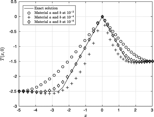
In this example, we assume that the exact initial data are known, albeit of the unknown exact temperature solution. They are given by piecewise smooth functions, as follows:$$\begin{array}{cc}\hfill T_b\left(x,0\right)=\left\{\begin{array}{cc}x,\hfill & x\in \left(-{\displaystyle \frac{b}{2}},0\right]\hfill \\ -{\displaystyle \frac{b}{2}},\hfill & x\in \left[-b,{\displaystyle \frac{b}{2}}\right]\hfill \end{array}\right.& \text{and}{T}_a\left(x,0\right)=\left\{\begin{array}{cc}-{\displaystyle \frac{a}{2}},\hfill & x\in \left({\displaystyle \frac{a}{2}},a\right],\hfill \\ -x,\hfill & x\in \left[0,{\displaystyle \frac{a}{2}}\right].\hfill \end{array}\right.\hfill \end{array}$$

Figure 3. The instability illustration with $\epsilon ={10}^{-2}$ at a cut-off high-frequency (selected randomly) $N=50$. (Example 4.1).

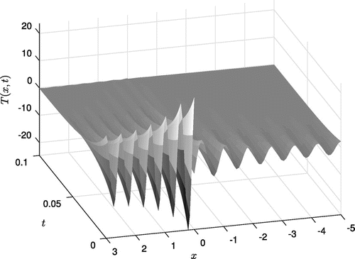
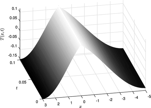
Figure 4. The stability illustration of the proposed cut-off projection, showing the approximate temperature throughout the two-slab system at $t_0=0$ with $\epsilon \in \left\{{10}^{-2},{10}^{-4},{10}^{-6}\right\}$. (Example 4.1).

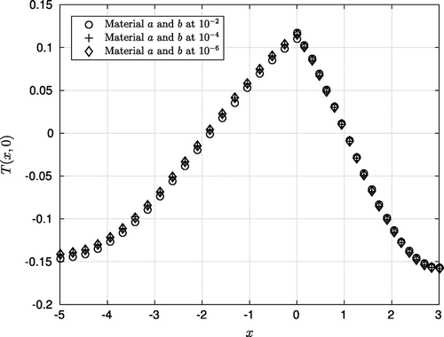
Figure 5. The approximate temperature throughout the two-slab system with $\epsilon ={10}^{-2}$ in a short-time observation. (Example 4.1).

In order to observe the approximation ${\mathbb{P}}_{\epsilon }{T}^{\epsilon }\left(x,t\right)$ to $T\left(x,t\right)$, the following steps are carried out:

(1)	Find the final values of $T_{\alpha }\left(x,t_f\right)$ from the forward problem which admits the solution expressed as: for $M\in \mathbb{N}$ (for comparison, we take $M=N_{\epsilon }$) $$T_{\alpha }\left(x,t\right)=\sum _{n=0}^M{\tilde{C}}_{\alpha n}{e}^{-{\overline{\lambda }}_{n}t}{\varphi }_{\alpha n}\left(x\right),$$ and to find ${\tilde{C}}_{\alpha n}$, we arrive at $$T_{\alpha }\left(x,t_0\right)=\sum _{n=0}^M{\tilde{C}}_{\alpha n}{\varphi }_{\alpha n}\left(x\right).$$
(2)	Obtain the values $T_{\alpha }^{\epsilon }\left(x,t_f\right)$ from those values of $T_{\alpha }\left(x,t_f\right)$ by perturbing them, as follows: $$\begin{array}{c}\hfill T_{\alpha }^{\epsilon }(x_j,t_f)=T_{\alpha }(x_j,t_f)+\text{rand}\left(x_j\right)\epsilon =\sum _{n=0}^M{\tilde{C}}_{\alpha n}{e}^{-{\overline{\lambda }}_n{t}_f}{\varphi }_{\alpha n}(x_j)+\text{rand}\left(x_j\right)\epsilon ,\end{array}$$ with $\left|\text{rand}\left(x_j\right)\right|\le {(2b)}^{-1/4}$ in order to fulfill (5(5) $$\begin{array}{c}\hfill {∥T_a\left(·,t_f\right)-T_a^{\epsilon }\left(·,t_f\right)∥}_{L^2\left(0,a\right)}+{∥T_b\left(·,t_f\right)-T_b^{\epsilon }\left(·,t_f\right)∥}_{L^2\left(-b,0\right)}\le \epsilon ,\end{array}$$(5) ).
(3)	Pass the resulting values to the approximate solution ${\mathbb{P}}_{\epsilon }{T}^{\epsilon }\left(x,t\right)$ in accordance with (25(25) $$\begin{array}{c}\hfill {\mathbb{P}}_{\epsilon }T(x,t)=\sum _{n\in \mathrm{\Theta }(\epsilon )}{C}_n{e}^{{\overline{\lambda }}_n\left(t_f-t\right)}{\tilde{\varphi }}_n\left(x\right),\end{array}$$(25) ) to find back the initial data $T_{\alpha }^{\epsilon }\left(x,t_0\right)$.

Similar steps are also used in Example 4.3 with the same type of noise. For our way of choosing $M=N_{\epsilon }$ in Step 1, this make things convenient since we can both obtain numerical results for the discrete exact solution and approximate solution with the same dimensions.

Figure 6. The comparison between the (artificial) exact initial data and the computed approximations at $t_0=0$ with $\epsilon \in \left\{{10}^{-2},{10}^{-4},{10}^{-6}\right\}$. (Example 4.2).

4.3. Example 3

We finalize this section by testing the example of Parker et al. [25] in which the prescribed initial data are provided by$$\left\{\begin{array}{cc}{T}_b\left(x,0\right)={\displaystyle \frac{Q}{{\rho }_b{c}_b\sigma }},\hfill & x\in \left(-b,0\right),\hfill \\ T_a\left(x,0\right)=0,\hfill & x\in \left(0,a\right),\hfill \end{array}\right.$$

where Q is the total heat energy in the initial pulse (cal$·{\text{cm}}^{-2}$) and the depth $\sigma$ at the front surface $x=-b$ is performed as a very small constant compared to the length $a+b$. These two dimensionless parameters will be selected as $Q=5$ and $\sigma ={10}^{-3}$.

Figure 7. The comparison (using log-scale for the y-axis) between the (artificial) exact initial data and the computed approximations at $t_0=0$ with $\epsilon \in \left\{{10}^{-2},{10}^{-4},{10}^{-6}\right\}$. (Example 4.3).

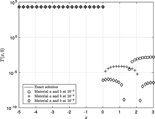
Table 1. Numerical results at $t_0=0$ with various different points in space.

Example 4.1
x	$\epsilon ={10}^{-2}$	$\epsilon ={10}^{-4}$	$\epsilon ={10}^{-6}$
$-$5	$-$0.14623	$-$0.14102	$-$0.14096
$-$2.63	$-$0.05644	$-$0.05122	$-$0.05117
1.42	$-$0.04657	$-$0.04891	$-$0.04889
3	$-$0.15609	$-$0.15843	$-$0.15841
Example 4.2
x	$\epsilon ={10}^{-2}$	$\epsilon ={10}^{-4}$	$\epsilon ={10}^{-6}$	Exact
$-$5	$-$2.49806	$-$2.50004	$-$2.5	$-$2.5
$-$2.63	$-$1.83030	$-$2.52717	$-$2.31534	$-$2.5
1.42	$-$1.02097	$-$1.48	$-$1.312359	$-$1.42105
3	$-$1.49997	$-$1.50005	$-$1.5	$-$1.5
Example 4.3
x	$\epsilon ={10}^{-2}$	$\epsilon ={10}^{-4}$	$\epsilon ={10}^{-6}$	Exact
$-$5	20405.73129	20405.72792	20405.72792	20405.72792
$-$2.63	20405.72961	20405.72797	20405.72792	20405.72792
1.42	0.00239	$-$2.22E$-$05	$-$3.41E$-$07	0
3	0.00159	4.53E$-$05	4.26E$-$07	0

4.4. Comments on numerical results

When approximating the temperature at $t_0=0$ for various amounts of noise $\epsilon \in \left\{{10}^{-2},{10}^{-4},{10}^{-6}\right\}$, we first observe in Figure 3 that the stability of solution ruins drastically for $\epsilon ={10}^{-2}$ for Example 4.1. Since in that example we do not have an analytical exact solution, the convergence of the scheme is affirmed by its stability (inspired from the Lax equivalence theorem). Thereby, it can be seen in Figure 4 that the approximation by the cut-off projection almost remains unchanged. For instance, at $(x,t)=(0,0)$ the approximation in the material a for $\epsilon ={10}^{-2}$ yields 0.11787, whilst the obtained values $\epsilon ={10}^{-4},{10}^{-6}$ are 0.11553 and 0.11556, respectively. As a result, the stable approximate solution has been depicted in Figure 5.

Aside from the first example, the measured final data in the next two examples is established from the artificial initial data by solving the direct problem. Then the approximations can be applied to find back the approximate initial data.

Figure 6 shows the accuracy of reconstructing the (artificial) exact initial data by the cut-off projection. In fact, we can observe a steady approach of the approximations (nodes) towards the exact solution (black line) as $\epsilon$ gets from ${10}^{-2}$ to ${10}^{-6}$. In line with that, Figure 7 also confirms a good approximation in the discontinuous case (Example 4.3).

In Table 1, numerical results with several different spatial points are provided. It is apparent that the numerical solutions in the nonsmooth and discontinuous cases are less stable (accurate) than that of the smooth example. It is simply because of the well-known Gibbs phenomenon, and that the reconstructed data near the nonsmooth and discontinuous points are not well-approximated. Nevertheless, taking into consideration the approximate values in Table 1 at the boundaries as well as the instability in Example 4.1 (Figure 3), the results in Example 4.2 and Example 4.3 are acceptable.

5. Discussion

5.1. Non-homogeneous case

We have successfully applied the cut-off method to solve the heat transfer problem backward in time in a 1D two-slab system with perfect contact. This system can be solved similarly when the heat source or sink is applied to the PDE. Indeed, let $F_{\alpha }:=F_{\alpha }\left(x,t\right)\in L^2\left(-b,a\right)$ represent the heat source or sink. The system (1(1) $$\begin{array}{cc}\hfill {\rho }_b{c}_b\frac{\partial T_b}{\partial t}& =K_b\frac{{\partial }^2{T}_b}{\partial x^2},-b<x<0,t\in J,\hfill \end{array}$$(1) )–(2(2) $$\begin{array}{cc}\hfill {\rho }_a{c}_a\frac{\partial T_a}{\partial t}& =K_a\frac{{\partial }^2{T}_a}{\partial x^2},0<x<a,t\in J.\hfill \end{array}$$(2) ) now reads(35) $$\begin{array}{c}\hfill {\rho }_b{c}_b\frac{\partial T_b}{\partial t}=K_b\frac{{\partial }^2{T}_b}{\partial x^2}+F_b,-b<x<0,t\in J,\end{array}$$(35) (36) $$\begin{array}{c}\hfill {\rho }_a{c}_a\frac{\partial T_a}{\partial t}=K_a\frac{{\partial }^2{T}_a}{\partial x^2}+F_a,0<x<a,t\in J.\end{array}$$(36)

As in Section 2, the system (35(35) $$\begin{array}{c}\hfill {\rho }_b{c}_b\frac{\partial T_b}{\partial t}=K_b\frac{{\partial }^2{T}_b}{\partial x^2}+F_b,-b<x<0,t\in J,\end{array}$$(35) )–(36(36) $$\begin{array}{c}\hfill {\rho }_a{c}_a\frac{\partial T_a}{\partial t}=K_a\frac{{\partial }^2{T}_a}{\partial x^2}+F_a,0<x<a,t\in J.\end{array}$$(36) ) together with the boundary conditions (3(3) $$\begin{array}{cc}\hfill \frac{\partial T_b}{\partial x}& =0\text{at}x=-b,\frac{\partial T_a}{\partial x}=0\text{at}x=a,t\in J\hfill \end{array}$$(3) )–(4(4) $$\begin{array}{cc}\hfill T_b& =T_a,K_b\frac{\partial T_b}{\partial x}=K_a\frac{\partial T_a}{\partial x}\text{at}x=0,t\in J.\hfill \end{array}$$(4) ) also lead to the transcendental conditions (10(10) $$\begin{array}{c}\hfill K_b{\lambda }_{b}sin\left({\lambda }_{b}b\right)cos\left({\lambda }_{a}a\right)+K_a{\lambda }_{a}sin\left({\lambda }_{a}a\right)cos\left({\lambda }_{b}b\right)=0.\end{array}$$(10) )–(11(11) $$\begin{array}{c}\hfill {\kappa }_b{\lambda }_b^2={\kappa }_a{\lambda }_a^2\end{array}$$(11) ), which allow direct computation of the eigenvalues ${\lambda }_{\mathit{an}},{\lambda }_{\mathit{bn}}$ and the eigenfunctions ${\varphi }_{\mathit{an}},{\varphi }_{\mathit{bn}}$ of the Sturm-Liouville equation. The temperature solution (in the finite series truncated computational sense) of the system (35(35) $$\begin{array}{c}\hfill {\rho }_b{c}_b\frac{\partial T_b}{\partial t}=K_b\frac{{\partial }^2{T}_b}{\partial x^2}+F_b,-b<x<0,t\in J,\end{array}$$(35) ),(36(36) $$\begin{array}{c}\hfill {\rho }_a{c}_a\frac{\partial T_a}{\partial t}=K_a\frac{{\partial }^2{T}_a}{\partial x^2}+F_a,0<x<a,t\in J.\end{array}$$(36) ), (3(3) $$\begin{array}{cc}\hfill \frac{\partial T_b}{\partial x}& =0\text{at}x=-b,\frac{\partial T_a}{\partial x}=0\text{at}x=a,t\in J\hfill \end{array}$$(3) ), (4(4) $$\begin{array}{cc}\hfill T_b& =T_a,K_b\frac{\partial T_b}{\partial x}=K_a\frac{\partial T_a}{\partial x}\text{at}x=0,t\in J.\hfill \end{array}$$(4) ) has the following form:(37) $$\begin{array}{cc}\hfill T(x,t)& =\sum _{n=0}^N\left[C_n{e}^{{\overline{\lambda }}_n(t_f-t)}-{\int }_t^{t_f}{D}_n(s)e^{{\overline{\lambda }}_n(s-t)}\mathrm{d}s\right]{\tilde{\varphi }}_n(x),\hfill \\ \hfill & (x,t)\in [-b,a]\times [t_0,t_f],\hfill \end{array}$$(37)

for some $N\in \mathbb{N}$. Here, we follow the notation ${\overline{\lambda }}_n={\kappa }_b{\lambda }_{\mathit{bn}}^2={\kappa }_a{\lambda }_{\mathit{an}}^2$ in Section 3, whilst the formula of ${\tilde{\varphi }}_n$ has already been introduced in (16(16) $$\begin{array}{c}\hfill {\tilde{\varphi }}_n(x)={\varphi }_{\mathit{bn}}(x)=\frac{cos\left({\lambda }_{\mathit{bn}}\left(x+b\right)\right)}{cos\left({\lambda }_{\mathit{bn}}b\right)}\text{for the left slab}\left(-b<x<0\right),\end{array}$$(16) )–(17(17) $$\begin{array}{c}\hfill {\tilde{\varphi }}_n(x)={\varphi }_{\mathit{an}}(x)=\frac{cos\left({\lambda }_{\mathit{an}}\left(x-a\right)\right)}{cos\left({\lambda }_{\mathit{an}}a\right)}\text{for the right slab}\left(0<x<a\right).\end{array}$$(17) ). The coefficients $C_n$ can be derived as in Section 3 from the final temperature condition (20(20) $$\begin{array}{c}\hfill T_N\left(x,t_f\right)=\sum _{n=0}^N{C}_n{\tilde{\varphi }}_n\left(x\right).\end{array}$$(20) ), while the algorithm for the time-dependent coefficient $D_{\alpha n}$ is rather difficult and can only be computed when $C_{\alpha n}$ are known. First of all, let us return to Equations (35(35) $$\begin{array}{c}\hfill {\rho }_b{c}_b\frac{\partial T_b}{\partial t}=K_b\frac{{\partial }^2{T}_b}{\partial x^2}+F_b,-b<x<0,t\in J,\end{array}$$(35) )–(36(36) $$\begin{array}{c}\hfill {\rho }_a{c}_a\frac{\partial T_a}{\partial t}=K_a\frac{{\partial }^2{T}_a}{\partial x^2}+F_a,0<x<a,t\in J.\end{array}$$(36) ) and then after plugging the representation (37(37) $$\begin{array}{cc}\hfill T(x,t)& =\sum _{n=0}^N\left[C_n{e}^{{\overline{\lambda }}_n(t_f-t)}-{\int }_t^{t_f}{D}_n(s)e^{{\overline{\lambda }}_n(s-t)}\mathrm{d}s\right]{\tilde{\varphi }}_n(x),\hfill \\ \hfill & (x,t)\in [-b,a]\times [t_0,t_f],\hfill \end{array}$$(37) ) into each quantity, we see that$$\begin{array}{cc}\hfill \frac{\partial T_{\alpha }}{\partial t}& =\sum _{n=0}^N\left[D_{\alpha n}\left(t\right)+{\overline{\lambda }}_n\left({\int }_t^{t_f}{D}_{\alpha n}\left(s\right)e^{{\overline{\lambda }}_n\left(s-t\right)}\mathrm{d}s-C_{\alpha n}{e}^{{\overline{\lambda }}_n\left(t_f-t\right)}\right)\right]{\varphi }_{\alpha n},\hfill \\ \hfill {\kappa }_{\alpha }\frac{{\partial }^2{T}_{\alpha }}{\partial x^2}& =-\sum _{n=0}^N{\overline{\lambda }}_n\left(C_{\alpha n}{e}^{{\overline{\lambda }}_n\left(t_f-t\right)}-{\int }_t^{t_f}{D}_{\alpha n}\left(s\right)e^{{\overline{\lambda }}_n\left(s-t\right)}\mathrm{d}s\right){\varphi }_{\alpha n},\hfill \\ \hfill \frac{\partial T_{\alpha }}{\partial t}& ={\kappa }_{\alpha }\frac{{\partial }^2{T}_{\alpha }}{\partial x^2}+\frac{1}{{\rho }_{\alpha }{c}_{\alpha }}{F}_{\alpha },\hfill \end{array}$$

where we have used the fundamental differentiation under the integral sign. Therefore, it follows that(38) $$\begin{array}{c}\hfill \sum _{n=0}^N{D}_{\alpha n}\left(t\right){\varphi }_{\alpha n}\left(x\right)=\frac{1}{{\rho }_{\alpha }{c}_{\alpha }}{F}_{\alpha }\left(x,t\right)\text{for}\alpha \in \left\{a,b\right\}.\end{array}$$(38)

As the second part of work, fix t in (38(38) $$\begin{array}{c}\hfill \sum _{n=0}^N{D}_{\alpha n}\left(t\right){\varphi }_{\alpha n}\left(x\right)=\frac{1}{{\rho }_{\alpha }{c}_{\alpha }}{F}_{\alpha }\left(x,t\right)\text{for}\alpha \in \left\{a,b\right\}.\end{array}$$(38) ) and once again, with the nodes ${\left\{x_j\right\}}_{j=\overline{0,J_{\alpha }}}$ it enables us to formulate the matrix-formed system $\mathbb{A}\mathbb{X}=\mathbb{B}$ then solve it through. Thereby, we have sufficient values for approximating the integral ${\displaystyle {\int }_t^{t_f}{D}_n\left(s\right)e^{{\overline{\lambda }}_n\left(s-t\right)}\mathrm{d}s}$, and that provides the way to numerically compute the temperature $T\left(x,t\right)$ by discrete nodes on the plane consisting of the time and spatial variables.

It is worthy noticing that $F_{\alpha }$ should satisfy the following condition so that (38(38) $$\begin{array}{c}\hfill \sum _{n=0}^N{D}_{\alpha n}\left(t\right){\varphi }_{\alpha n}\left(x\right)=\frac{1}{{\rho }_{\alpha }{c}_{\alpha }}{F}_{\alpha }\left(x,t\right)\text{for}\alpha \in \left\{a,b\right\}.\end{array}$$(38) ) is solvable:$$\frac{1}{{\rho }_a{c}_a}{〈F_a(x,t),{\varphi }_{\mathit{an}}(x)〉}_{L^2(0,a)}=\frac{1}{{\rho }_b{c}_b}{〈F_b(x,t),{\varphi }_{\mathit{bn}}(x)〉}_{L^2(-b,0)}\text{for all}n\in \mathbb{N}.$$

The above condition is a necessary condition for $F_{\alpha }$. We do not aim at finding the sufficient condition to guarantee the existence of solution of the system (35(35) $$\begin{array}{c}\hfill {\rho }_b{c}_b\frac{\partial T_b}{\partial t}=K_b\frac{{\partial }^2{T}_b}{\partial x^2}+F_b,-b<x<0,t\in J,\end{array}$$(35) )–(36(36) $$\begin{array}{c}\hfill {\rho }_a{c}_a\frac{\partial T_a}{\partial t}=K_a\frac{{\partial }^2{T}_a}{\partial x^2}+F_a,0<x<a,t\in J.\end{array}$$(36) ) in this manuscript.

5.2. The bilayer system in 2D

In this subsection, we generalize the homogeneous problem to two dimensional space. We consider the backward heat transfer problem between two plates: the left plate is the rectangle $[-b,0]\times [0,c]$, while the right plate is $[0,a]\times [0,c]$. The heat distribution in the time interval $[t_0,t_f]$ is described by:(39) $$\begin{array}{cc}\hfill {\rho }_b{c}_b\frac{\partial T_b}{\partial t}& =K_b\mathrm{\Delta }{T}_b,\left(x,y\right)\in \left(-b,0\right)\times \left(0,c\right),t\in J,\hfill \end{array}$$(39) (40) $$\begin{array}{cc}\hfill {\rho }_a{c}_a\frac{\partial T_a}{\partial t}& =K_a\mathrm{\Delta }{T}_a,\left(x,y\right)\in \left(0,a\right)\times \left(0,c\right),t\in J.\hfill \end{array}$$(40)

Unlike the problem (1(1) $$\begin{array}{cc}\hfill {\rho }_b{c}_b\frac{\partial T_b}{\partial t}& =K_b\frac{{\partial }^2{T}_b}{\partial x^2},-b<x<0,t\in J,\hfill \end{array}$$(1) )–(2(2) $$\begin{array}{cc}\hfill {\rho }_a{c}_a\frac{\partial T_a}{\partial t}& =K_a\frac{{\partial }^2{T}_a}{\partial x^2},0<x<a,t\in J.\hfill \end{array}$$(2) ), we have the boundary conditions on each side of the rectangle and also at the intersection of them, i.e. $\left(x,y\right)\in \left\{0\right\}\times [0,c]$,(41) $$\begin{array}{c}\hfill \frac{\partial T_b}{\partial x}=0\text{at}x=-b,\frac{\partial T_a}{\partial x}=0\text{at}x=a,t\in J,\end{array}$$(41) $$\frac{\partial T_b}{\partial y}=0\text{at}\left(x,y\right)\in [-b,0]\times \left\{0,c\right\},\frac{\partial T_a}{\partial y}=0\text{at}\left(x,y\right)\in [0,a]\times \left\{0,c\right\},t\in J,$$ (42) $$\begin{array}{c}\hfill T_b=T_a,K_b\frac{\partial T_b}{\partial x}=K_a\frac{\partial T_a}{\partial x}\text{at}\left(x,y\right)\in \left\{0\right\}\times [0,c],t\in J.\end{array}$$(42)

Using the same approach as in Section 2, we can construct the eigen-elements as the solution of(43) $$\begin{array}{c}\hfill \mathrm{\Delta }{\varphi }_{\alpha }\left(x,y\right)+{\lambda }_{\alpha }^2{\varphi }_{\alpha }\left(x,y\right)=0\text{for}\alpha \in \left\{a,b\right\},\end{array}$$(43)

with the assumption that the time dependence of each plates is the same, and that ${\varphi }_{\alpha }$ inherits the boundary conditions (41(41) $$\begin{array}{c}\hfill \frac{\partial T_b}{\partial x}=0\text{at}x=-b,\frac{\partial T_a}{\partial x}=0\text{at}x=a,t\in J,\end{array}$$(41) )–(42(42) $$\begin{array}{c}\hfill T_b=T_a,K_b\frac{\partial T_b}{\partial x}=K_a\frac{\partial T_a}{\partial x}\text{at}\left(x,y\right)\in \left\{0\right\}\times [0,c],t\in J.\end{array}$$(42) ).

We apply the separation variable technique for (43(43) $$\begin{array}{c}\hfill \mathrm{\Delta }{\varphi }_{\alpha }\left(x,y\right)+{\lambda }_{\alpha }^2{\varphi }_{\alpha }\left(x,y\right)=0\text{for}\alpha \in \left\{a,b\right\},\end{array}$$(43) ) by assuming that ${\varphi }_{\alpha }\left(x,y\right)$ can be expressed as ${\varphi }_{\alpha }\left(x,y\right)=X_{\alpha }\left(x\right)Y_{\alpha }\left(y\right)$. Then, (43(43) $$\begin{array}{c}\hfill \mathrm{\Delta }{\varphi }_{\alpha }\left(x,y\right)+{\lambda }_{\alpha }^2{\varphi }_{\alpha }\left(x,y\right)=0\text{for}\alpha \in \left\{a,b\right\},\end{array}$$(43) ) becomes(44) $$\begin{array}{c}\hfill {\displaystyle \frac{X_{\alpha }^{″}}{X_{\alpha }}}+{\lambda }_{\alpha }^2=-{\displaystyle \frac{Y_{\alpha }^{″}}{Y_{\alpha }}}={\mu }_{\alpha }^2.\end{array}$$(44)

Direct computation yields that $Y_{\alpha }(y)={\eta }_{\alpha }cos({\mu }_{\alpha }y)$, where ${\eta }_{\alpha }=\sqrt{{\displaystyle \frac{2}{c}}}$ is a constant and ${\mu }_{\alpha }=\mu ={\displaystyle \frac{m\pi }{c}}$ for $m\in \mathbb{N}$. Since we are solely interested in the case ${\lambda }_{\alpha }^2>{\mu }_{\alpha }^2$, we can assume that ${\nu }_{\alpha }^2={\lambda }_{\alpha }^2-{\mu }_{\alpha }^2$. In the same manner with Section 2, we obtain$$X_a={\theta }_{a}cos\left({\nu }_a\left(x-a\right)\right);X_b={\theta }_{b}cos\left({\nu }_b\left(x+b\right)\right),$$

where ${\theta }_a,{\theta }_b$ are constants. The transcendental condition (10(10) $$\begin{array}{c}\hfill K_b{\lambda }_{b}sin\left({\lambda }_{b}b\right)cos\left({\lambda }_{a}a\right)+K_a{\lambda }_{a}sin\left({\lambda }_{a}a\right)cos\left({\lambda }_{b}b\right)=0.\end{array}$$(10) ) now reads(45) $$\begin{array}{c}\hfill K_b{\nu }_{b}sin\left({\nu }_{b}b\right)cos\left({\nu }_{a}a\right)+K_a{\nu }_{a}sin\left({\nu }_{a}a\right)cos\left({\nu }_{b}b\right)=0.\end{array}$$(45)

Similarly, a 2D version of condition (11(11) $$\begin{array}{c}\hfill {\kappa }_b{\lambda }_b^2={\kappa }_a{\lambda }_a^2\end{array}$$(11) ) is(46) $$\begin{array}{c}\hfill {\kappa }_a\left({\nu }_a^2+{\mu }_a^2\right)={\kappa }_b\left({\nu }_b^2+{\mu }_b^2\right).\end{array}$$(46)

The temperature solution of the system (39(39) $$\begin{array}{cc}\hfill {\rho }_b{c}_b\frac{\partial T_b}{\partial t}& =K_b\mathrm{\Delta }{T}_b,\left(x,y\right)\in \left(-b,0\right)\times \left(0,c\right),t\in J,\hfill \end{array}$$(39) )–(40(40) $$\begin{array}{cc}\hfill {\rho }_a{c}_a\frac{\partial T_a}{\partial t}& =K_a\mathrm{\Delta }{T}_a,\left(x,y\right)\in \left(0,a\right)\times \left(0,c\right),t\in J.\hfill \end{array}$$(40) ) together with the boundary conditions (41(41) $$\begin{array}{c}\hfill \frac{\partial T_b}{\partial x}=0\text{at}x=-b,\frac{\partial T_a}{\partial x}=0\text{at}x=a,t\in J,\end{array}$$(41) )–(42(42) $$\begin{array}{c}\hfill T_b=T_a,K_b\frac{\partial T_b}{\partial x}=K_a\frac{\partial T_a}{\partial x}\text{at}\left(x,y\right)\in \left\{0\right\}\times [0,c],t\in J.\end{array}$$(42) ) is$$T_{\alpha }\left(x,y,t\right)=\sum _{m,n\ge 0}{C}_{\alpha mn}{e}^{{\kappa }_{\alpha }\left({\nu }_{\alpha n}^2+{\mu }_{\alpha m}^2\right)\left(t_f-t\right)}{X}_{\alpha n}\left(x\right)Y_{\alpha m}\left(y\right),$$

where the coefficient $C_{\alpha mn}$ can be derived from the temperature distribution at the final time:$$T_{\alpha }(x,y,t_f)=\sum _{m,n\ge 0}{C}_{\alpha mn}{X}_{\alpha n}\left(x\right)Y_{\alpha m}\left(y\right).$$

For the time being, the algorithm proposed in Section 2 can be applied again in searching for the eigenvalues ${\left\{{\nu }_{\alpha n}\right\}}_{n\in \mathbb{N}}$ which are solutions to (45(45) $$\begin{array}{c}\hfill K_b{\nu }_{b}sin\left({\nu }_{b}b\right)cos\left({\nu }_{a}a\right)+K_a{\nu }_{a}sin\left({\nu }_{a}a\right)cos\left({\nu }_{b}b\right)=0.\end{array}$$(45) ) and (46(46) $$\begin{array}{c}\hfill {\kappa }_a\left({\nu }_a^2+{\mu }_a^2\right)={\kappa }_b\left({\nu }_b^2+{\mu }_b^2\right).\end{array}$$(46) ). Note from (46(46) $$\begin{array}{c}\hfill {\kappa }_a\left({\nu }_a^2+{\mu }_a^2\right)={\kappa }_b\left({\nu }_b^2+{\mu }_b^2\right).\end{array}$$(46) ) that if the thermal diffusivities of two plates are identical (i.e. ${\kappa }_a={\kappa }_b$), it turns back to solving the system (14(14) $$\begin{array}{c}\hfill \frac{K_b}{\sqrt{{\kappa }_b}}sin\left({\lambda }_{b}b\right)cos\left(\sqrt{\frac{{\kappa }_b}{{\kappa }_a}}{\lambda }_{b}a\right)+\frac{K_a}{\sqrt{{\kappa }_a}}sin\left(\sqrt{\frac{{\kappa }_b}{{\kappa }_a}}{\lambda }_{b}a\right)cos\left({\lambda }_{b}b\right)=0,\end{array}$$(14) )–(15(15) $$\begin{array}{c}\hfill {\lambda }_a=\sqrt{\frac{{\kappa }_b}{{\kappa }_a}}{\lambda }_b\end{array}$$(15) ).

Applying again the cut-off projection, our regularized solution in the 2D two-slab system is given by$$T^{\epsilon }(x,y,t)=\sum _{m,n\in \mathrm{\Theta }(\epsilon )}{C}_{\mathit{mn}}{e}^{{\overline{\lambda }}_{\mathit{mn}}(t_f-t)}{X}_n(x)Y_m(y),$$

associated with the terminal measured data $T_{\alpha }^{\epsilon }\left(x,y,t_f\right)$ satisfying(47) $$\begin{array}{c}\hfill {∥T_a\left(·,t_f\right)-T_a^{\epsilon }\left(·,t_f\right)∥}_{L^2\left((0,a)\times (0,c)\right)}+{∥T_b\left(·,t_f\right)-T_b^{\epsilon }\left(·,t_f\right)∥}_{L^2\left((-b,0)\times (0,c)\right)}\le \epsilon .\end{array}$$(47)

Here, the set of admissible frequencies is defined by $\mathrm{\Theta }(\epsilon ):=\left\{(m,n)\in {\mathbb{N}}^2:{\overline{\lambda }}_{\mathit{mn}}\le N_{\epsilon }\right\}$ with ${\overline{\lambda }}_{\mathit{mn}}:={\kappa }_a\left({\nu }_{\mathit{an}}^2+{\mu }_{\mathit{am}}^2\right)={\kappa }_b\left({\nu }_{\mathit{bn}}^2+{\mu }_{\mathit{bm}}^2\right)$.

Taking again ${\kappa }_{\alpha }\in \left\{0.838,0.339\right\}$ and $K_{\alpha }\in \left\{3.42,1.05\right\}$ as in Section 4, we test the cut-off projection with a simple 2D problem in a normalized square two-slab system, i.e. $a=b=c=1$, and with $t_f=0.1$, $\beta =0.01$, $\gamma =1$.

In this test, since the values of thermal diffusivities are known, we are allowed to write from (46(46) $$\begin{array}{c}\hfill {\kappa }_a\left({\nu }_a^2+{\mu }_a^2\right)={\kappa }_b\left({\nu }_b^2+{\mu }_b^2\right).\end{array}$$(46) ) that(48) $$\begin{array}{c}\hfill {\nu }_a=\sqrt{\frac{{\kappa }_b}{{\kappa }_a}{\nu }_b^2+\left(\frac{{\kappa }_b}{{\kappa }_a}-1\right){\mu }^2},\end{array}$$(48)

and thus get the transcendental condition in (45(45) $$\begin{array}{c}\hfill K_b{\nu }_{b}sin\left({\nu }_{b}b\right)cos\left({\nu }_{a}a\right)+K_a{\nu }_{a}sin\left({\nu }_{a}a\right)cos\left({\nu }_{b}b\right)=0.\end{array}$$(45) ) that(49) $$\begin{array}{cc}& K_b{\nu }_{b}sin({\nu }_{b}b)cos\left(a\sqrt{\frac{{\kappa }_b}{{\kappa }_a}{\nu }_b^2+\left(\frac{{\kappa }_b}{{\kappa }_a}-1\right){\mu }^2}\right)\hfill \\ \hfill & +K_a\sqrt{\frac{{\kappa }_b}{{\kappa }_a}{\nu }_b^2+\left(\frac{{\kappa }_b}{{\kappa }_a}-1\right){\mu }^2}sin\left(a\sqrt{\frac{{\kappa }_b}{{\kappa }_a}{\nu }_b^2+\left(\frac{{\kappa }_b}{{\kappa }_a}-1\right){\mu }^2}\right)cos({\nu }_{b}b)=0.\hfill \end{array}$$(49)

As we can see from (49(49) $$\begin{array}{cc}& K_b{\nu }_{b}sin({\nu }_{b}b)cos\left(a\sqrt{\frac{{\kappa }_b}{{\kappa }_a}{\nu }_b^2+\left(\frac{{\kappa }_b}{{\kappa }_a}-1\right){\mu }^2}\right)\hfill \\ \hfill & +K_a\sqrt{\frac{{\kappa }_b}{{\kappa }_a}{\nu }_b^2+\left(\frac{{\kappa }_b}{{\kappa }_a}-1\right){\mu }^2}sin\left(a\sqrt{\frac{{\kappa }_b}{{\kappa }_a}{\nu }_b^2+\left(\frac{{\kappa }_b}{{\kappa }_a}-1\right){\mu }^2}\right)cos({\nu }_{b}b)=0.\hfill \end{array}$$(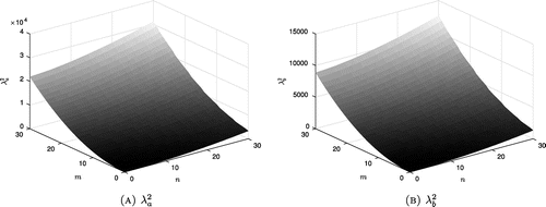49) ) , the eigenvalues cannot be computed directly. In order to depict the behavior of those eigenvalues, we demonstrate a simple numerical example by giving an exact smooth form of initial data, viz.$$\begin{array}{cc}\hfill T_b\left(x,y,0\right)=cos\left(\pi \left(x+b\right)\right)cos\left(\pi y\right),& T_a\left(x,y,0\right)=cos\left(\pi \left(x-a\right)\right)cos\left(\pi y\right).\hfill \end{array}$$

Notice that these are the initial values for the forward problem. Following the steps mentioned in Section 4.2, we set the limit of our summation in the expression of Fourier form solution, i.e. $(m,n)\in \mathrm{\Theta }(\epsilon )$ and calculate the eigenvalues according to (48(48) $$\begin{array}{c}\hfill {\nu }_a=\sqrt{\frac{{\kappa }_b}{{\kappa }_a}{\nu }_b^2+\left(\frac{{\kappa }_b}{{\kappa }_a}-1\right){\mu }^2},\end{array}$$(48) ) and (49(49) $$\begin{array}{cc}& K_b{\nu }_{b}sin({\nu }_{b}b)cos\left(a\sqrt{\frac{{\kappa }_b}{{\kappa }_a}{\nu }_b^2+\left(\frac{{\kappa }_b}{{\kappa }_a}-1\right){\mu }^2}\right)\hfill \\ \hfill & +K_a\sqrt{\frac{{\kappa }_b}{{\kappa }_a}{\nu }_b^2+\left(\frac{{\kappa }_b}{{\kappa }_a}-1\right){\mu }^2}sin\left(a\sqrt{\frac{{\kappa }_b}{{\kappa }_a}{\nu }_b^2+\left(\frac{{\kappa }_b}{{\kappa }_a}-1\right){\mu }^2}\right)cos({\nu }_{b}b)=0.\hfill \end{array}$$(49) ). In Figure 8, we compute several numerical eigenvalues driven by (48(48) $$\begin{array}{c}\hfill {\nu }_a=\sqrt{\frac{{\kappa }_b}{{\kappa }_a}{\nu }_b^2+\left(\frac{{\kappa }_b}{{\kappa }_a}-1\right){\mu }^2},\end{array}$$(48) ) and (49(49) $$\begin{array}{cc}& K_b{\nu }_{b}sin({\nu }_{b}b)cos\left(a\sqrt{\frac{{\kappa }_b}{{\kappa }_a}{\nu }_b^2+\left(\frac{{\kappa }_b}{{\kappa }_a}-1\right){\mu }^2}\right)\hfill \\ \hfill & +K_a\sqrt{\frac{{\kappa }_b}{{\kappa }_a}{\nu }_b^2+\left(\frac{{\kappa }_b}{{\kappa }_a}-1\right){\mu }^2}sin\left(a\sqrt{\frac{{\kappa }_b}{{\kappa }_a}{\nu }_b^2+\left(\frac{{\kappa }_b}{{\kappa }_a}-1\right){\mu }^2}\right)cos({\nu }_{b}b)=0.\hfill \end{array}$$(49) ) by using the built-in function fzero from MATLAB (this has already been introduced in Section 2).

In this example we consider the system at $y_0=0$. The algorithm for this 2D case is similar to that for the 1D case (see in Section 4). Basically, the following steps are carried out:

(1)	Find the final values from the forward problem $$\begin{array}{c}\hfill T_{\alpha }(x,y_0,t)=\sum _{m,n\in \mathrm{\Theta }(\epsilon )}{\tilde{C}}_{\alpha mn}{e}^{-{\overline{\lambda }}_{n}t}{X}_{\alpha n}(x)Y_m(y_0),\end{array}$$ and to find ${\tilde{C}}_{\alpha mn}$, we solve a linear system $\mathbb{A}\mathbb{X}=\mathbb{B}$ where $$\mathbb{A}=\left[\begin{array}{cccc}{X}_{\alpha 0}(x_0)Y_0(y_0)& X_{\alpha 0}(x_0)Y_1(y_0)& \dots & X_{\alpha n}(x_0)Y_m(y_0)\\ X_{\alpha 0}(x_1)Y_0(y_0)& X_{\alpha 0}(x_0)Y_1(y_0)& \dots & X_{\alpha n}(x_1)Y_m(y_0)\\ ⋮& ⋮& \ddots & ⋮\\ X_{\alpha 0}(x_{J_{\alpha }})Y_0(y_0)& X_{\alpha 0}(x_{J_{\alpha }})Y_1(y_0)& \dots & X_{\alpha n}(x_{J_{\alpha }})Y_m(y_0)\end{array}\right]\in {\mathbb{R}}^{{(J_{\alpha }+1)}^2},$$ $$\mathbb{X}=\left[\begin{array}{c}{\tilde{C}}_{\alpha 00}\\ {\tilde{C}}_{\alpha 01}\\ ⋮\\ {\tilde{C}}_{\alpha nm}\end{array}\right]\in {\mathbb{R}}^{J_{\alpha }+1},\mathbb{B}=\left[\begin{array}{c}{T}_{\alpha }(x_0,y_0,t_0)\\ T_{\alpha }(x_1,y_0,t_0)\\ ⋮\\ T_{\alpha }(x_{J_{\alpha }},y_0,t_0)\end{array}\right]\in {\mathbb{R}}^{J_{\alpha }+1}.$$ In this case we choose $J_{\alpha }=\left|\mathrm{\Theta }(\epsilon )\right|-1$ where $\left|\mathrm{\Theta }(\epsilon )\right|$ is the cardinality of $\mathrm{\Theta }(\epsilon )$.
(2)	Obtain the values $T_{\alpha }^{\epsilon }\left(x,y_0,t_f\right)$ from those values of $T_{\alpha }\left(x,y_0,t_f\right)$ by perturbing them, as follows: $$\begin{array}{cc}\hfill T_{\alpha }^{\epsilon }(x_j,y_0,t_f)& =T_{\alpha }(x_j,y_0,t_f)+\text{rand}\left(x_j\right)\epsilon \hfill \\ \hfill & =\sum _{m,n\in \mathrm{\Theta }(\epsilon )}{\tilde{C}}_{\alpha mn}{e}^{-{\overline{\lambda }}_n{t}_f}{X}_{\alpha n}(x)Y_m(y_0)+\text{rand}\left(x_j\right)\epsilon ,\hfill \end{array}$$ with $\left|\text{rand}\left(x_j\right)\right|\le {((a+b)c)}^{-1/2}$.
(3)	Perform the proposed method on generated data to find back the initial data $T_{\alpha }^{\epsilon }\left(x,y_0,t_0\right)$.

Figure 8. Numerical eigenvalues ${\lambda }_{\alpha }^2={\nu }_{\alpha }^2+{\mu }_{\alpha }^2$ for the two-slab system in 2D at $\epsilon ={10}^{-6}$.

Figure 9. The comparison between the (artificial) exact initial data and the computed approximations at $y_0=0,t_0=0$ with $\epsilon \in \left\{{10}^{-2},{10}^{-4},{10}^{-6}\right\}$. (Example for a two-slab system in 2D).

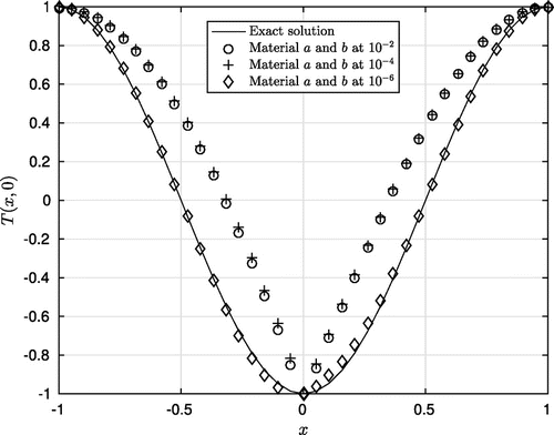
We have drawn in Figure 9 the numerical results of the exact initial data and the computed approximations based on our proposed cut-off projection at $y_0=0$ and at $t_0=0$. We can easily observe that these approximations (colored nodes) are closer to the exact initial data (black line) as $\epsilon$ goes from ${10}^{-2}$ to ${10}^{-6}$. This corroborates that our theoretical analysis works well in this 2D example and thus implies the applicability of the proposed method in higher dimensions.

5.3. Boundary conditions

So far, we merely have considered the two-slab problem under idealistic conditions, such as the system has a perfect contact, there is no heat entering or escaping at the boundary of the two slabs. More realistic conditions should be more interesting, for example, an imperfect contact or Robin-type condition motivated by Newton’s Law of Cooling. However, the more complicated boundary conditions, the more severe difficulties of computation we have, especially for the eigen-elements. We shall leave detailed studies of such realistic models for further research.

Acknowledgements

V.A.K. acknowledges Prof. Errico Presutti (GSSI, Italy) for his invaluable help during the PhD years. The authors wish to express their sincere thanks to the anonymous referees and the associate editors for many constructive comments leading to the improved versions of this paper.

Disclosure statement

No potential conflict of interest was reported by the authors.

Additional information

Funding

This work is supported by the Institute for Computational Science and Technology (Ho Chi Minh city) under project named ‘Some ill-posed problems for partial differential equations’ [312/Q -KHCNTT].

References

- Lattès R, Lions J. Méthode de Quasi-réversibilité et Applications. Paris: Dunod; 1967.
- Buzbee B, Carasso A. On the numerical computation of parabolic problems for preceding times. Math Comput. 1973;27(122):237–266.
- Clark G, Oppenheimer S. Quasireversibility methods for non-well-posed problems. Elect J Differ Equ. 1994;1994(8):1–9.
- Denche M, Bessila K. A modified quasi-boundary value method for ill-posed problems. J Math Anal Appl. 2005;301:419–426.
- Hào D, Duc N, Sahli H. A non-local boundary value problem method for parabolic equations backward in time. J Math Anal Appl. 2008;345:805–815.
- Seidman T. Optimal filtering for the backward heat equation. SIAM J Numer Anal. 1996;33(1):162–170.
- Trong D, Tuan N. A nonhomogeneous backward heat problem: regularization and error estimates. Elect J Differ Equ. 2008;2008(33):1–14.
- Lesnic D, Elliott L, Ingham D. An iterative boundary element method for solving the backward heat conduction problem using an elliptic approximation. Inverse Probl Eng. 1998;6(4):255–279.
- Johansson B, Lesnic D, Reeve T. A method of fundamental solutions for radially symmetric and axisymmetric backward heat conduction problems. Int J Comput Math. 2012;89(11):1555–1568.
- Hào D, Duc N, Lesnic D. Regularization of parabolic equations backward in time by a non-local boundary value problem method. IMA J Appl Math. 2010;75(2):291–315.
- Lesnic D. The decomposition method for forward and backward time-dependent problems. J Comput Appl Math. 2002;147(1):27–39.
- Mei C, Vernescu B. Homogenization methods for multiscale mechanics. Singapore: World Scientific Publishing; 2010.
- Ternat F, Daripa P, Orellana O. On an inverse problem: recovery of non-smooth solutions to backward heat equation. Appl Math Model. 2012;36:4003–4019.
- Ternat F, Orellana O, Daripa P. Two stable methods with numerical experiments for solving the backward heat equation. Appl Numer Math. 2011;61:266–284.
- Regińska T, Regiński K. Approximate solution of a Cauchy problem for the Helmholtz equation. Inverse Probl. 2006;22:975–989.
- Tuan N, Khoa V, Minh M, et al. Reconstruction of the electric field of the Helmholtz equation in three dimensions. J Comput Appl Math. 2017;309:56–78.
- Ortega J, Rheinboldt W. Iterative solution of nonlinear equations in several variables. New York: Academic Press; 1970.
- Cordero A, Torregrosa J. Variants of Newton’s method using fifth-order quadrature formulas. Appl Math Comput. 2007;190:686–698.
- Noor M, Waseem M. Some iterative methods for solving a system of nonlinear equations. Comput Math Appl. 2009;57(1):101–106.
- Josell D, Cezairliyan A, van Heerden D, et al. Thermal diffusion through multilayer coatings: theory and experiment. Nanostruct Mater. 1997;9:727–736.
- Nam P, Trong D, Tuan N. The truncation method for a two-dimensional nonhomogeneous backward heat problem. Appl Math Comput. 2010;216:3423–3432.
- Tuan N, Au V, Khoa V, et al. Identification of the population density of a species model with nonlocal diffusion and nonlinear reaction. Inverse Probl. 2017;33(5):055019.
- Mera N, Elliott L, Ingham D, et al. An iterative boundary element method for solving the one-dimensional backward heat conduction problem. Int J Heat Mass Transfer. 2001;44(10):1937–1946.
- Johansson B, Lesnic D, Reeve T. A comparative study on applying the method of fundamental solutions to the backward heat conduction problem. Math Comput Model. 2011;54(1–2):403–416.
- Parker W, Jenkins R, Butler C, et al. Flash method of determining thermal diffusivity, heat capacity and thermal conductivity. J Appl Phys. 1961;32(9):1679–1684.