Material model calibration for superplastic forming

ABSTRACT

Superplastic forming is a slow forming process. The forming time can be minimized by optimizing the pressure profile applied to the forming sheet. The optimization of the superplastic forming pressure is usually done such that a target strain rate at a high strain rate sensitivity is maintained. Careful consideration of the strain rate is required, since localized thinning can occur when the material is strained too quickly. This paper demonstrates that it is essential to explicitly include strain rate sensitivity data, obtained from strain rate jump tests, during the calibration of material model used for superplastic forming simulations. Conventional calibration methods only consider stress–strain data at different strain rates. Such an approach implicitly assumes that a material model that matches the stress–strain data at the different strain rates, will automatically match strain rate sensitivity data. However, by explicitly including the strain rate sensitivity data, the selected material model is more susceptible to localized thinning as the applied strain rate is increased. It is essential for the selected material model to exhibit this behaviour to prevent superplastic forming simulations at high strain rates from predicting stable deformation, when in fact localized thinning will occur.

KEYWORDS:

• Material model
• superplastic forming
• strain rate sensitivity
• finite element method
• optimization

MSC SUBJECT CLASSIFICATION:

• 74C20

1. Introduction

Superplasticity is the almost neck-free elongation of several hundreds of per cent that can be observed in some metals when a metal with certain metallurgical properties is strained at a certain strain rate and temperature. These metallurgical properties usually include small, equiaxed grains that are typically less than $10\text{μ}\mathrm{m}$ in diameter. Ti-6Al-4V exhibits superplastic behaviour at strain rates less than ${10}^{-3}$ s⁻¹ at temperatures greater than 900${}^{\circ }$C [1].

The relationship between logarithmic flow stress and logarithmic strain rate for superplastic metals at high temperatures during uniaxial tensile tests has a sigmoid shape [2,3]. The sigmoid curve, depicted in Figure 1, is divided into three strain rate regions where region II is the superplastic strain rate region.

Figure 1. Sigmoid relationship between $\log \sigma$ and $\log \dot{\epsilon }$.

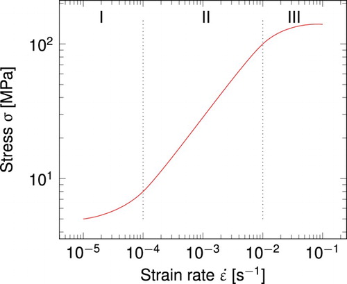
The strain rate sensitivity m is defined as the slope of the sigmoid curve, which is given by [4] (1) $m=\frac{\mathrm{\partial }\log \sigma }{\mathrm{\partial }\log \dot{\epsilon }}.$(1) Region II has the highest strain rate sensitivity, and the strain rate sensitivity decreases in the higher strain rate region III [4].

The two factors that control superplastic failure under any selected test conditions are the strain rate sensitivity, which dominates localized thinning, and the cavity formation [5]. Localized thinning usually occurs in the higher strain rate regions II to III. Cavitation failure is not investigated in this study.

The optimization of the superplastic forming pressure is usually done such that a target strain rate in region II is maintained [6,7]. This approach to optimizing superplastic forming is unnecessarily restrictive, since a high strain rate sensitivity is not required during the first stages of forming [8].

This paper demonstrates the implementation and calibration of a superplastic material model. The importance of including strain rate sensitivity data in the calibration of the superplastic material model in order to predict the onset of localized thinning is highlighted.

2. Material model

2.1. Implementation

Three material models that can be used to describe superplastic behaviour are implemented into Abaqus using user creep subroutines. The first model is denoted as the SV-sinh (state variable-based hyperbolic sine) model, where the equivalent creep strain rate $\dot{\epsilon }$ of the SV-sinh model is given by [9] (2) $\dot{\epsilon }={\alpha }_2\sinh \left({\beta }_2\left(\sigma -R-k\right)\right)d^{-\gamma }.$(2) Here σ is equivalent stress, d is grain size, and R is the isotropic hardening. The rate of isotropic hardening of the superplastic material is given by [9] (3) $\dot{R}=b(Q-R)\dot{\epsilon }.$(3) The grain growth model is given by (4) $\dot{d}={\alpha }_1{d}^{-{\gamma }_0}+{\beta }_1\dot{\epsilon }{d}^{-\phi }.$(4) Here ${\alpha }_2$, ${\beta }_2$, k, γ, b, Q, ${\alpha }_1$, ${\gamma }_0$, ${\beta }_1$ and φ are constants to be determined through calibration with data.

The second material model is denoted as Lin's model, which is similar to the SV-sinh model, except that it has a less flexible grain growth model, which is given by [9] (5) $\dot{d}=\left({\alpha }_1+{\beta }_1\dot{\epsilon }\right)d^{-\phi }.$(5)

The third material model is a model that can be found in the paper by Nazzal et al. [10], and it denoted as the Nazzal model in this study. The equivalent creep strain rate $\dot{\epsilon }$ of the Nazzal model is given by (6) $\dot{\epsilon }=\frac{C_i}{d^p}{\left(\frac{\sigma }{1-f_{a0}\exp \left(\psi \epsilon \right)}-{\sigma }_0\right)}^{1/q}+C_{ii}{\left(\frac{\sigma }{1-f_{a0}\exp \left(\psi \epsilon \right)}\right)}^r.$(6) The grain growth is described by [10] (7) $\dot{d}=\frac{k_{\mathrm{s}}}{d^g}+\frac{k_{\mathrm{d}}}{d^g}\left(1-\exp \left(\frac{-t}{\tau }\right)\right)\dot{\epsilon },$(7) where t is time. The constants $C_i$, p, $f_{a0}$, ψ, ${\sigma }_0$, q, $C_{ii}$, r, $k_{\mathrm{s}}$, g, $k_{\mathrm{d}}$ and τ also have to be determined through calibration with data.

The equivalent plastic strain increment $\mathrm{\Delta }{\epsilon }_{\mathrm{p}}$ and its derivative with respect to equivalent stress $\mathrm{d}\mathrm{\Delta }{\epsilon }_{\mathrm{p}}/\mathrm{d}\sigma$ and strain $\mathrm{d}\mathrm{\Delta }{\epsilon }_{\mathrm{p}}/\mathrm{d}\epsilon$ have to be updated in the creep user subroutine when implicit integration is used. The inputs to the subroutine include the initial conditions to the state variables, the equivalent stress and strain at the start and at the end of the increment, and the time and the time increment $\mathrm{\Delta }t$. The state variables of the SV-sinh model and Lin's model are the isotropic hardening variable R and the grain size d. The state variable of the Nazzal model is grain size d.

There is viscoplastic flow when $\sigma \ge (k+R)$ in Equation (2(2) $\dot{\epsilon }={\alpha }_2\sinh \left({\beta }_2\left(\sigma -R-k\right)\right)d^{-\gamma }.$(2) ), otherwise $\mathrm{\Delta }{\epsilon }_{\mathrm{p}}$ and $\mathrm{d}\mathrm{\Delta }\epsilon /\mathrm{d}\sigma$ are equal to zero, and R and d remain unchanged. If there is viscoplastic flow, in other words when $\sigma \ge (k+R)$ in the case of the SV-sinh model, the increment in plastic strain $\mathrm{\Delta }{\epsilon }_{\mathrm{p}}$ can be calculated using the implicit trapezoidal integration method (8) $\mathrm{\Delta }{\epsilon }_{\mathrm{p}}=\frac{\mathrm{\Delta }t}{2}\left({\dot{\epsilon }}_{n+1}+{\dot{\epsilon }}_n\right),$(8) where ${\dot{\epsilon }}_n$ is the current strain rate and ${\dot{\epsilon }}_{n+1}$ is the strain rate of the next iteration. The state variables have to be updated before ${\dot{\epsilon }}_{n+1}$ can be calculated. The state variables can be updated using the Newton–Raphson method which is given by (9) $\frac{\mathrm{d}\mathbf{R}\mathbf{e}\mathbf{s}}{\mathrm{d}\mathit{y}}\mathrm{\Delta }\mathit{y}=-\mathbf{R}\mathbf{e}\mathbf{s}.$(9) In the case of the SV-sinh model and Lin's model, $\mathit{y}$ and $\mathrm{\Delta }\mathit{y}$ is given by (10) $\mathit{y}=\left\{\begin{array}{c}{R}_{n+1}\\ d_{n+1}\end{array}\right\},$(10) and (11) $\mathrm{\Delta }\mathit{y}=\left\{\begin{array}{c}\mathrm{\Delta }R\\ \mathrm{\Delta }d\end{array}\right\},$(11) respectively. $\mathbf{R}\mathbf{e}\mathbf{s}$ contains the residual of the state variables, and in the case of the SV-sinh model and Lin's model it is given by (12) $\mathbf{R}\mathbf{e}\mathbf{s}=\left\{\begin{array}{c}{\mathrm{Res}}_R\\ {\mathrm{Res}}_d\end{array}\right\}.$(12) The system Jacobian $\mathrm{d}\mathbf{R}\mathbf{e}\mathbf{s}/\mathrm{d}\mathit{y}$ in Equation (9(9) $\frac{\mathrm{d}\mathbf{R}\mathbf{e}\mathbf{s}}{\mathrm{d}\mathit{y}}\mathrm{\Delta }\mathit{y}=-\mathbf{R}\mathbf{e}\mathbf{s}.$(9) ) for the case of the SV-sinh and Lin's model is given by (13) $\frac{\mathrm{d}\mathbf{R}\mathbf{e}\mathbf{s}}{\mathrm{d}\mathit{y}}=\left[\begin{array}{cc}\frac{\mathrm{\partial }{\mathrm{Res}}_R}{\mathrm{\partial }{R}_{n+1}}& \frac{\mathrm{\partial }{\mathrm{Res}}_R}{\mathrm{\partial }{d}_{n+1}}\\ \frac{\mathrm{\partial }{\mathrm{Res}}_d}{\mathrm{\partial }{R}_{n+1}}& \frac{\mathrm{\partial }{\mathrm{Res}}_d}{\mathrm{\partial }{d}_{n+1}}\end{array}\right].$(13) In the case of the Nazzal model, Equation (9(9) $\frac{\mathrm{d}\mathbf{R}\mathbf{e}\mathbf{s}}{\mathrm{d}\mathit{y}}\mathrm{\Delta }\mathit{y}=-\mathbf{R}\mathbf{e}\mathbf{s}.$(9) ) can be rewritten as (14) $\frac{\mathrm{d}\mathbf{R}\mathbf{e}\mathbf{s}}{\mathrm{d}d}\mathrm{\Delta }d=-{\mathrm{Res}}_d.$(14) The residuals ${\mathrm{Res}}_d$ and ${\mathrm{Res}}_R$ can be found using the implicit trapezoidal method, where ${\mathrm{Res}}_R$ is given by (15) ${\mathrm{Res}}_R=R_{n+1}-R_n-\frac{\mathrm{\Delta }t}{2}\left({\dot{R}}_{n+1}+{\dot{R}}_n\right),$(15) and ${\mathrm{Res}}_d$ is given by (16) ${\mathrm{Res}}_d=d_{n+1}-d_n-\frac{\mathrm{\Delta }t}{2}\left({\dot{d}}_{n+1}+{\dot{d}}_n\right).$(16)

Next, the derivative of the equivalent plastic strain increment with respect to equivalent stress $\mathrm{d}\mathrm{\Delta }\epsilon /\mathrm{d}{\sigma }_{n+1}$ has to be calculated. It can be found using the chain rule of differentiation. In the case of the SV-sinh model and Lin's model, it is given by (17) $\frac{\mathrm{d}\mathrm{\Delta }\epsilon }{\mathrm{d}{\sigma }_{n+1}}=\frac{\mathrm{\partial \Delta }\epsilon }{\mathrm{\partial }{\sigma }_{n+1}}+\frac{\mathrm{\partial \Delta }\epsilon }{\mathrm{\partial }{R}_{n+1}}\frac{\mathrm{d}{R}_{n+1}}{\mathrm{d}{\sigma }_{n+1}}+\frac{\mathrm{\partial \Delta }\epsilon }{\mathrm{\partial }{d}_{n+1}}\frac{\mathrm{d}{d}_{n+1}}{\mathrm{d}{\sigma }_{n+1}}.$(17) The derivatives $\mathrm{d}{R}_{n+1}/\mathrm{d}{\sigma }_{n+1}$ and $\mathrm{d}{d}_{n+1}/\mathrm{d}{\sigma }_{n+1}$ in Equation (17(17) $\frac{\mathrm{d}\mathrm{\Delta }\epsilon }{\mathrm{d}{\sigma }_{n+1}}=\frac{\mathrm{\partial \Delta }\epsilon }{\mathrm{\partial }{\sigma }_{n+1}}+\frac{\mathrm{\partial \Delta }\epsilon }{\mathrm{\partial }{R}_{n+1}}\frac{\mathrm{d}{R}_{n+1}}{\mathrm{d}{\sigma }_{n+1}}+\frac{\mathrm{\partial \Delta }\epsilon }{\mathrm{\partial }{d}_{n+1}}\frac{\mathrm{d}{d}_{n+1}}{\mathrm{d}{\sigma }_{n+1}}.$(17) ) can be found using the Newton–Raphson method (18) $\frac{\mathrm{d}\mathbf{R}\mathbf{e}\mathbf{s}}{\mathrm{d}\mathit{y}}\frac{\mathrm{d}\mathit{y}}{\mathrm{d}{\sigma }_{n+1}}=-\frac{\mathrm{\partial }\mathbf{R}\mathbf{e}\mathbf{s}}{\mathrm{\partial }{\sigma }_{n+1}}.$(18)

In the case of the Nazzal model, $\mathrm{d}\mathrm{\Delta }\epsilon /\mathrm{d}{\sigma }_{n+1}$ is calculated using the chain rule of differentiation (19) $\frac{\mathrm{d}\mathrm{\Delta }\epsilon }{\mathrm{d}{\sigma }_{n+1}}=\frac{\mathrm{\partial \Delta }\epsilon }{\mathrm{\partial }{\sigma }_{n+1}}+\frac{\mathrm{\partial \Delta }\epsilon }{\mathrm{\partial }{d}_{n+1}}\frac{\mathrm{d}{d}_{n+1}}{\mathrm{d}{\sigma }_{n+1}},$(19) where $\mathrm{d}{d}_{n+1}/\mathrm{d}{\sigma }_{n+1}$ is given by (20) $\frac{\mathrm{d}{\mathrm{Res}}_d}{\mathrm{d}d}\frac{\mathrm{d}d}{\mathrm{d}{\sigma }_{n+1}}=-\frac{\mathrm{\partial }{\mathrm{Res}}_d}{\mathrm{\partial }{\sigma }_{n+1}}.$(20)

The derivative of the equivalent plastic strain increment with respect to equivalent stress $\mathrm{d}\mathrm{\Delta }\epsilon /\mathrm{d}{\epsilon }_{n+1}$ is also calculated using the chain rule of differentiation (21) $\frac{\mathrm{d}\mathrm{\Delta }\epsilon }{\mathrm{d}{\epsilon }_{n+1}}=\frac{\mathrm{\partial \Delta }\epsilon }{\mathrm{\partial }{\epsilon }_{n+1}}+\frac{\mathrm{\partial \Delta }\epsilon }{\mathrm{\partial }{d}_{n+1}}\frac{\mathrm{d}{d}_{n+1}}{\mathrm{d}{\epsilon }_{n+1}},$(21) where the derivative $\mathrm{d}{d}_{n+1}/\mathrm{d}{\epsilon }_{n+1}$ in Equation (21(21) $\frac{\mathrm{d}\mathrm{\Delta }\epsilon }{\mathrm{d}{\epsilon }_{n+1}}=\frac{\mathrm{\partial \Delta }\epsilon }{\mathrm{\partial }{\epsilon }_{n+1}}+\frac{\mathrm{\partial \Delta }\epsilon }{\mathrm{\partial }{d}_{n+1}}\frac{\mathrm{d}{d}_{n+1}}{\mathrm{d}{\epsilon }_{n+1}},$(21) ) is given by (22) $\frac{\mathrm{d}{\mathrm{Res}}_d}{\mathrm{d}{d}_{n+1}}\frac{\mathrm{d}{d}_{n+1}}{\mathrm{d}{\epsilon }_{n+1}}=-\frac{\mathrm{\partial }{\mathrm{Res}}_d}{\mathrm{\partial }{\epsilon }_{n+1}}.$(22)

The subroutine can be tested as a standalone routine by also computing the equivalent stress increment $\mathrm{\Delta }\sigma$ using the Newton–Raphson method (23) $\frac{\mathrm{d}\mathrm{\Delta }\epsilon }{\mathrm{d}\sigma }\mathrm{\Delta }\sigma =-{\mathrm{Res}}_{\sigma },$(23) where ${\mathrm{Res}}_{\sigma }$ is given by (24) ${\mathrm{Res}}_{\sigma }=\mathrm{\Delta }\epsilon -\mathrm{\Delta }{\epsilon }_{\mathrm{target}}.$(24) The total strain increment $\mathrm{\Delta }\epsilon$ is the sum of its elastic $\mathrm{\Delta }{\epsilon }_{\mathrm{e}}$ and plastic $\mathrm{\Delta }{\epsilon }_{\mathrm{p}}$ components, where the elastic strain increment $\mathrm{\Delta }{\epsilon }_{\mathrm{e}}$ is given by (25) $\mathrm{\Delta }{\epsilon }_{\mathrm{e}}=\frac{\sigma }{E},$(25) and E is Young's modulus. The plastic component is calculated in the subroutine. The target strain increment $\mathrm{\Delta }{\epsilon }_{\mathrm{target}}$ is given by (26) $\mathrm{\Delta }{\epsilon }_{\mathrm{target}}=\mathrm{\Delta }t{\dot{\epsilon }}_{\mathrm{target}},$(26) where ${\dot{\epsilon }}_{\mathrm{target}}$ is the target strain rate.

2.2. Calibration

Published stress–strain, strain rate sensitivity-strain and grain size-time data were used to calibrate the SV-sinh model. The strain rate sensitivity is critical to predict localized thinning at higher strain rates [11,12]. It will be shown in this study exactly how critical it is to calibrate a superplastic material model using all of the available data.

The published data, digitized from the experimental work by Ghosh and Hamilton [11], is for Ti-6Al-4V with three initial grain sizes strained at different strain rates at a temperature of 927${}^{\circ }$C. Ghosh and Hamilton [11] found the strain rate sensitivity-strain data using strain rate jump tests.

The calibration of the material models is stated as an optimization problem where the objective function $f\left(\mathit{x}\right)$ to be minimized is given by (27) $f\left(\mathit{x}\right)=e_{\mathrm{T}}=e_{\sigma }+w_m{e}_m+w_d{e}_d,$(27) where $\mathit{x}$ is the material constants that have to be determined, $e_{\mathrm{T}}$ is the total error, $e_{\sigma }$ is the stress error, $e_m$ is the strain rate sensitivity error, and $e_d$ is the grain size error. The strain rate sensitivity error weight and grain size error weight is given by $w_m$ and $w_d$, respectively. This weighted sum method always yields a minimum that is Pareto optimal if the weights are positive [13]. The objective function is minimized using the Nelder–Mead simplex method.

The strain rate sensitivity error $e_m$ and grain size error $e_d$ are each calculated using the root of the square error, for example, $e_m$ is given by (28) $e_m=\sqrt{\sum _{i=1}^k{\left(m_i-m_i^{\mathrm{data}}\right)}^2}.$(28)

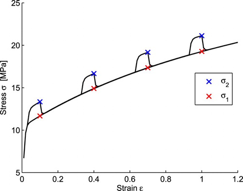
The strain rate sensitivity m is calculated using a numerical strain rate jump test. The numerical strain rate jump test starts off at a constant strain rate $\dot{\epsilon }$ s⁻¹. The strain rate is then increased to $1.25\dot{\epsilon }$ s⁻¹ and held there for approximately 2–$3\mathrm{\%}$ plastic strain. The strain rate is then decreased back to $\dot{\epsilon }$. An example of a strain rate jump test is shown in Figure 2. The stress just before the decrease from $1.25\dot{\epsilon }$ s⁻¹ is given by ${\sigma }_2$, and the stress at $\dot{\epsilon }$ at the corresponding total strain is given by ${\sigma }_1$. The strain rate sensitivity m is therefore given by (29) $\begin{array}{r}m=\frac{\log \left({\sigma }_2/{\sigma }_1\right)}{\log \left(1.25\right)}.\end{array}$(29) More detail on strain rate jump tests is given in the relevant ASTM standard [14].

Figure 2. Numerical strain rate jump test.

3. Results

3.1. Calibration

Three sets of error weights w = {w_m, w_d} were investigated for the SV-sinh model. The optimized parameters ${\mathit{x}}_{\mathrm{opt}}=\{Y,{\beta }_2,k,a_2,b,Q,a_1,{\beta }_1,Y_0,\varphi \}$, final errors $\mathit{e}=\{e_{\sigma },e_m,e_d\}$ and total error $e_{\mathrm{T}}$ for these weights are given in Table 1. The weights of set 1 favour the stress–strain data more than the strain rate sensitivity-strain data and grain size-time data, and the strain rate sensitivity-strain data is effectively ignored (this last error contributes less than 0.2% to the total error). The weights of set 2 favour the strain rate sensitivity-strain data more than the other data sets. The weights of set 3 attempt to balance the stress error and strain rate sensitivity error.

Table 1. Optimized parameters for three sets of arbitrary weights for the SV-sinh model.

Set	$\mathit{w}$	${\mathit{x}}_{\mathrm{opt}}$	$\mathit{e}$	$e_{\mathrm{T}}$
		2.3079
		0.11325
		$1.3318\times {10}^{-17}$
1	1	0.04818	82.185
	1	1.5114	0.17902	110.35
		5.2662	27.988
		0.85654
		1.8277
		3.7841
		0.12167
		2.9162
		0.11952
		$2.64\times {10}^{-17}$
2	24,000	0.14636	524.77
	10.8	0.32491	0.030841	1581.4
		3.8655	29.297
		8.9568
		1.8241
		4.8116
		$6.4877\times {10}^{-8}$
		2.4253
		0.11532
		$1.5603\times {10}^{-15}$
		0.057089	125.14
3	1500	1.033	0.09296	342.41
	2.7	4.5091	28.827
		9.0249
		1.7347
		4.8029
		$6.9144\times {10}^{-20}$

The SV-sinh model calibrated with to the three different sets of weights is compared to the published data in Figures 3– 5.

Figure 3. The SV-sinh model with $\mathit{w}=\left\{11\right\}$ (set 1) fitted to (a) stress–strain data, (b) strain rate sensitivity-strain data, and grain size-time data in (c), (d) and (e).

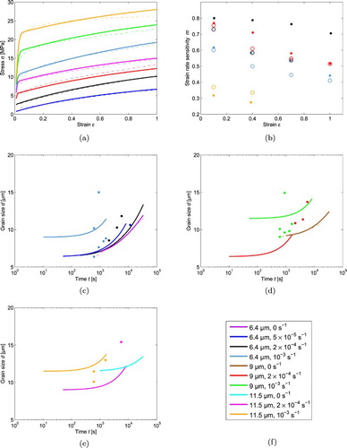
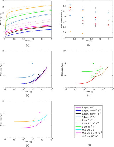
Figure 4. The SV-sinh model with $\mathit{w}=\left\{2400010.8\right\}$ (set 2) fitted to (a) stress–strain data, (b) strain rate sensitivity-strain data, and grain size-time data in (c), (d) and (e).

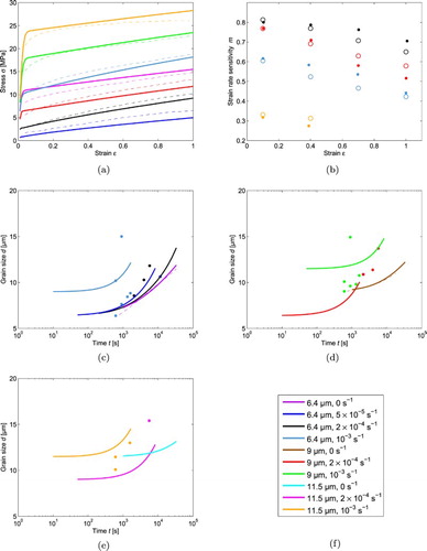
Figure 5. The SV-sinh model with $\mathit{w}=\left\{15002.7\right\}$ (set 3) fitted to (a) stress–strain data, (b) strain rate sensitivity-strain data, and grain size-time data in (c), (d) and (e).

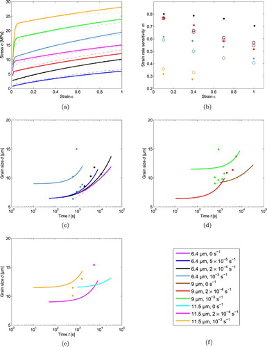
Notice in Figure 3 that the SV-sinh model describes all the stress–strain data well, but not the strain rate sensitivity data. In particular, notice that the strain rate sensitivity of the $6.4\text{μ}\mathrm{m}$ material is less than that of the $9\text{μ}\mathrm{m}$ material, when in fact it should be the other way round. In Figure 4 all the strain rate sensitivity data is fitted well, but the quality of fit of the stress–strain data is compromised.

The grain size errors for all three sets are almost the same. It is however difficult to judge the fit of the dynamic grain size-time experimental data, because there are large error bars on the dynamic grain size-time data given by Ghosh and Hamilton [11].

Lin used a genetic algorithm to calibrate his model to the same published data [9]. The material parameters of Lin's model is given by [9] (30) ${\mathit{x}}_{\mathrm{opt}}=\left\{\begin{array}{c}\gamma \\ {\beta }_2\\ k\\ {\alpha }_2\\ b\\ Q\\ {\alpha }_1\\ {\beta }_1\\ {\gamma }_0\end{array}\right\}=\left\{\begin{array}{c}1.408\\ 0.035\\ 0.242\\ 0.042\\ 1.729\\ 6.345\\ 1.2\\ 3460.5\\ 3.7\end{array}\right\}.$(30)

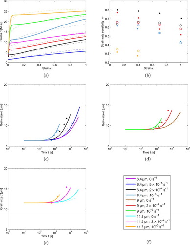
Lin's model is compared to the published stress–strain, strain rate sensitivity-strain and grain size-time data in Figure 6. Lin's model is only calibrated with stress–strain and grain size-time data with an initial grain size of $6.4\text{μ}\mathrm{m}$ [9]. The consequence is that the stress–strain experimental data with initial grain sizes other than $6.4\text{μ}\mathrm{m}$ are not captured in the calibration. This is evident in Figure 6.

Figure 6. Lin's model compared to published (a) stress–strain data, (b) strain rate sensitivity-strain data, and grain size-time data in (c), (d) and (e).

Lin does not incorporate strain rate sensitivity-strain experimental data in the calibration of his model. The consequence is that that the strain rate sensitivity-strain model data does not match the strain rate sensitivity-strain experimental data in Figure 6(b).

Two sets of error weights were investigated for the Nazzal model. The optimized parameters ${\mathit{x}}_{\mathrm{opt}}=\{C_i,C_{ii},q,r,p,g,\psi ,T,F_{a0},k_s,k_d,{\sigma }_0\}$, final errors $\mathit{e}$ and total error $e_{\mathrm{T}}$ for these weights are given in Table 2. The weights $\mathit{w}=\left\{11\right\}$ effectively ignores the strain rate sensitivity data, while the weights $\mathit{w}=\left\{6002.27\right\}$ attempt to balance the stress error and strain rate sensitivity error.

Table 2. Optimized parameters to two sets of arbitrary weights for the Nazzal model.

$\mathit{w}$	${\mathit{x}}_{\mathrm{opt}}$	$\mathit{e}$	$e_{\mathrm{T}}$
	0.0015673
	$1.2795\times {10}^{-9}$
	0.62622
	3.7779
	2.3253	141.54
1	0.71504	0.30015	210.64
1	0.0069727	68.805
	370.42
	0.00086761
	30.35
	0.0028445
	0.0045786
	0.0018378
	$8.3316\times {10}^{-13}$
	0.6848
	5.8073
	2.4039	209.9
600	1.6043	0.095587	360.56
2.27	0.00043915	41.102
	708.94
	0.0063218
	248.05
	0.20933
	$7.1734\times {10}^{-6}$

The Nazzal model calibrated with the two different sets of weights is compared to the published data in Figures 7 and  8. The strain rate sensitivity-strain data is described better by the SV-sinh model as compared to the Nazzal model for weights $\mathit{w}=\left\{11\right\}$.The grain growth of the Nazzal model shown in Figures 7 and  8 is faster than the grain growth of the SV-sinh model and Lin's model.

Figure 7. The Nazzal model with $\mathit{w}=\left\{11\right\}$ fitted to (a) stress–strain data, (b) strain rate sensitivity-strain data, and grain size-time data in (c), (d) and (e).

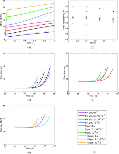
Figure 8. The Nazzal model with $\mathit{w}=\left\{6002.27\right\}$ fitted to (a) stress–strain data, (b) strain rate sensitivity-strain data, and grain size-time data in (c), (d) and (e).

3.2. Finite element tensile test model

The different material models are compared by modelling the tensile tests that generated the stress–strain curves. The ability of the different material models to predict the earlier onset of necking as the applied strain rate is increased is of particular interest. If the material models do not predict this behaviour, such models would not be suitable to optimize pressure profiles during superplastic forming.

The geometry and dimensions of the tensile test specimen are from Ghosh and Hamilton [11]. The test specimen is 1.63 mm thick. The tensile test model is meshed with four layers of C3D8 elements. The meshed tensile test model is shown in Figure 9. The mesh is graded to be finer in the gauge area, and it is finer towards the middle of the gauge section. This mesh grading is necessary to maintain good mesh quality towards the end of the simulations, where elongations of up to 250% are required to investigate if localized deformation will occur. Our numerical experiments have indicated that this mesh density is adequate to ensure mesh independent results [15].

Figure 9. The tensile test model.

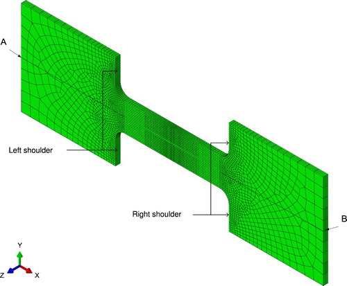
The boundary conditions of the tensile test model are based on the ASTM standard [14]. The top and bottom surfaces of the tabs cannot displace in the y-direction. The middle line along the leftmost and rightmost surfaces cannot displace in the z-direction. The left shoulder cannot displace in the x-direction. A velocity boundary condition is applied to the right shoulder of the specimen. The magnitude of the velocity boundary condition is given by [11,14] (31) $v=L_0\dot{\epsilon }\exp \left(\dot{\epsilon }t\right),$(31) where $L_0$ is the initial gauge length and t is the time from the start of the test. The applied velocity boundary condition is supposed to be such that a constant strain rate is maintained throughout the gauge section [11]. Strain rates of ${10}^{-3}$ s⁻¹, $2\times {10}^{-3}$ s⁻¹ and $5\times {10}^{-3}$ s⁻¹ are used in the study. The initial grain size is set to $6.4\text{μ}\mathrm{m}$.

The final thickness results from point A to point B for the finite element model with the different material models at three different strain rates are given in Figure 10. It can be observed that almost all of the deformation is in the gauge section for all the models investigated.

Figure 10. Final thickness results along the middle of the tensile test specimen at a strain rate of (a) ${10}^{-3}$ s⁻¹, (b) $2\times {10}^{-3}$ s⁻¹ and (c) $5\times {10}^{-3}$ s⁻¹.

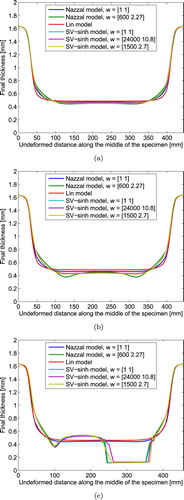
The thickness results are non-uniform in the gauge section for all three sets of the SV-sinh model and for the Nazzal model with $\mathit{w}=\left\{6002.27\right\}$ at $2\times {10}^{-3}$ s⁻¹ and $5\times {10}^{-3}$ s⁻¹ in Figure 10(b,c), respectively. The results of Lin's model and the Nazzal model with $\mathit{w}=\left\{11\right\}$ show no localized thinning at or near the end of the $2\times {10}^{-3}$ s⁻¹ and $5\times {10}^{-3}$ s⁻¹ simulations. Recall that Lin did not use strain rate sensitivity data to calibrate his material model. The calibration of the Nazzal model with $\mathit{w}=\left\{11\right\}$ did however incorporate strain rate sensitivity-strain data, but the strain rate sensitivity data was not captured with this set of weights. The strain rate sensitivity error of the Nazzal model with $\mathit{w}=\left\{11\right\}$ is three times more than the strain rate sensitivity error of the Nazzal model with $\mathit{w}=\left\{6002.27\right\}$.

The maximum principal strain rate along the middle of the tensile test model increased over time for all the tensile test models. The maximum principal strain rate versus the normalized deformed distance along the middle of the tensile test model for set 3 of the SV-sinh model at ${10}^{-3}$ s⁻¹ is shown in Figure 11. The increase in strain rate in the gauge section is 57% from 10 s to 2480 s in this case. This may be due to considerable flow of material from the tabs to the gauge section that increases with time. Material flows from the tabs to the gauge section, because the material is less resistive to flow at high temperature. The flow of material from the tabs has been observed in real superplastic tensile tests [16].

Figure 11. Maximum principal strain rate along the middle of the tensile test model with time for set 3 of the SV-sinh model at ${10}^{-3}$ s⁻¹.

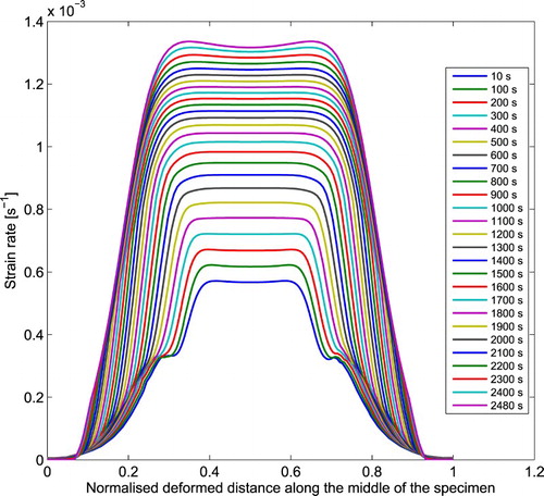
The flow of material from the tabs influences the stress–strain measurements. This is a possible explanation of the inconsistency between the implied strain rate sensitivities from the stress–strain curves, as compared to the strain rate sensitivities obtained from strain rate jump tests. This also justifies an approach where the stress–strain data is not considered as more important than the strain rate sensitivity data during calibration. Inverse modelling of the tensile test can be done to calibrate the material model in order to account for the varying strain rate throughout the gauge section with time [17], but this approach is beyond the scope of the current paper.

In summary, all three versions of the calibrated SV-sinh model and the Nazzal model with $\mathit{w}=\left\{6002.27\right\}$ show the onset of localized thinning with increasing strain rate. These models would be suitable to minimize the final forming time of a superplastic forming process, by finding a pressure profile that forms the part faster, subject to some minimum allowable thickness. An optimization algorithm that uses the material model calibrated in this paper would naturally avoid pressures that deform the part too quickly, since this would lead to localization [15].

4. Conclusion

The SV-sinh model and the Nazzal model are successfully calibrated with published stress–strain data, grain size-time data and strain rate sensitivity-strain data using a weighted sum optimization strategy. The thickness results indicate localized thinning in the gauge section for all three weight sets of the SV-sinh model and for the Nazzal model with $\mathit{w}=\left\{6002.27\right\}$ at strain rates of $2\times {10}^{-3}$ s⁻¹ and $5\times {10}^{-3}$ s⁻¹. The Nazzal model with $\mathit{w}=\left\{11\right\}$ showed no localized thinning at or near the end of the $2\times {10}^{-3}$ s⁻¹ and $5\times {10}^{-3}$ s⁻¹ simulations. The Nazzal model with $\mathit{w}=\left\{11\right\}$ incorporated strain rate sensitivity-strain data in the calibration process, but the strain rate sensitivity data was not captured with this set of weights. The strain rate sensitivity error of the Nazzal model with $\mathit{w}=\left\{11\right\}$ is three times more than the strain rate sensitivity error of the Nazzal model with $\mathit{w}=\left\{6002.27\right\}$.

These models were compared to a model by Lin, which is similar to the SV-sinh model, with the exception that it has a less flexible grain growth model than the SV-sinh model. Lin calibrated his model only to stress–strain and grain size-time experimental data with an initial grain size of $6.4\text{μ}\mathrm{m}$ [9]. He did not make use of data with different initial grain sizes, and he did not use strain rate sensitivity-strain data to calibrate the model. It was shown that this calibration of Lin's model consequently did not show localized thinning with increasing strain rate for the finite element tensile test model. A material model should therefore not only be fitted to data of only one grain size and strain rate if the material model is going to be used in multi-axial simulations. This is because the material model needs to provide an adequate description for many grain sizes and strain rates during a multi-axial simulation. This happens when some parts of the sheet are in contact with the die and other parts are still forming into the die cavity.

The velocity boundary condition was assumed to lead to a constant strain rate in the gauge section. However, it was found that the maximum principal strain rate increased with time. This might be due to material flow from the tabs. This is also a possible explanation of the inconsistency between the implied strain rate sensitivities from the stress–strain curves, as compared to the strain rate sensitivities obtained from strain rate jump tests. This also justifies an approach where the stress–strain data is not considered as more important than the strain rate sensitivity data during calibration.

Disclosure statement

No potential conflict of interest was reported by the authors.

References

- Velay V, Matsumoto H, Vidal V, et al. Behavior modeling and microstructural evolutions of Ti6Al4V alloy under hot forming conditions. Int J Mech Sci. 2016;108-109:1–13 [cited 2016 Mar 11]. Available from: http://dx.doi.org/10.1016/j.ijmecsci.2016.01.024
- Bonet J, Gil A, Wood RD, et al. Simulating superplastic forming. Comput Methods Appl Mech Eng. 2006;195(48–49):6580–6603. doi: 10.1016/j.cma.2005.03.012
- Kruglov AA, Ganieva VR, Tulupova OP, et al. Computational methods of the superplastic forming duration of a round membrane. Russ J Non-Ferrous Met. 2017;58(3):250–257. doi: 10.3103/S1067821217030099
- Alabort E, Kontis P, Barba D, et al. On the mechanisms of superplasticity in Ti-6Al-4V. Acta Mater. 2016;105:449–463 [cited 2016 Jan 22]. Available from: http://dx.doi.org/10.1016/j.actamat.2015.12.003
- Alabort E, Putman D, Reed RC. Superplasticity in Ti-6Al-4V: characterisation, modelling and applications. Acta Mater. 2015;95:428–442. doi: 10.1016/j.actamat.2015.04.056
- Wang Y, Mishra RS. Finite element simulation of selective superplastic forming of friction stir processed 7075 Al alloy. Mater Sci Eng A. 2007;463(1–2):245–248. doi: 10.1016/j.msea.2006.08.118
- Sheikhalishahi H, Farzin M. A new approach for determining the optimum pressuretime diagram in superplastic forming process. Int J Adv Des Manuf Technol. 2014;6(3):71–76.
- Bate PS, Ridley N, Zhang B, et al. Optimisation of the superplastic forming of aluminium alloys. J Mater Process Technol. 2006;177(1–3):91–94. doi: 10.1016/j.jmatprotec.2006.03.200
- Lin J. Selection of material models for predicting necking in superplastic forming. Int J Plast. 2002;19(4):469–481. doi: 10.1016/S0749-6419(01)00059-6
- Nazzal MA, Khraisheh MK, Darras BM. Finite element modeling and optimization of superplastic forming using variable strain rate approach. J Mater Eng Perform. 2004;13(6):691–699 [cited 2017 Jan 31]. Available from: https://link.springer.com/article/10.1361/10599490421321
- Ghosh AK, Hamilton CH. Mechanical behavior and hardening characteristics of a superplastic Ti-6Al-4V alloy. Metallur Trans A. 1979;10(6):699–706. doi: 10.1007/BF02658391
- Nazzal M, Khraisheh M, Abu-Farha F. The effect of strain rate sensitivity evolution on deformation stability during superplastic forming. J Mater Process Technol. 2007;191(1–3):189–192. doi: 10.1016/j.jmatprotec.2007.03.097
- Arora JS. Introduction to optimum design. 3rd ed. Waltham: Academic Press; 2012.
- ASTM E2448-11 Standard test method for determining the superplastic properties of metallic sheet; 2011.
- Cowley MS. Optimising pressure profiles in superplastic forming. M Eng thesis University of Pretoria; 2017.
- Abu-Farha FK. Integrated approach to the superplastic forming of magnesium alloys. Doctor of philosophy. University of Kentucky; 2007. Available from: http://uknowledge.uky.edu/gradschool_diss/493/http://uknowledge.uky.edu/gradschool_diss/493/.
- Cooreman S, Lecompte D, Sol H, et al. Identification of mechanical material behavior through inverse modeling and DIC. Exp Mech. 2008;48:421–433.