
 ?Mathematical formulae have been encoded as MathML and are displayed in this HTML version using MathJax in order to improve their display. Uncheck the box to turn MathJax off. This feature requires Javascript. Click on a formula to zoom.
ABSTRACT
The parameters of many physical processes are unknown and have to be inferred from experimental data. The corresponding parameter estimation problem is often solved using iterative methods such as steepest descent methods combined with trust regions. For a few problem classes also continuous analogues of iterative methods are available. In this work, we expand the application of continuous analogues to function spaces and consider PDE (partial differential equation)-constrained optimization problems. We derive a class of continuous analogues, here coupled ODE (ordinary differential equation)–PDE models, and prove their convergence to the optimum under mild assumptions. We establish sufficient bounds for local stability and convergence for the tuning parameter of this class of continuous analogues, the retraction parameter. To evaluate the continuous analogues, we study the parameter estimation for a model of gradient formation in biological tissues. We observe good convergence properties, indicating that the continuous analogues are an interesting alternative to state-of-the-art iterative optimization methods.
1. Introduction
Partial differential equations (PDEs) are used in various application areas to describe physical, chemical, biological, economic, or social processes. The parameters of these processes are often unknown and need to be estimated from experimental data [Citation1,Citation2]. The maximum likelihood and maximum a posteriori parameter estimates are given by the solutions of PDE-constrained optimization problems. Since PDE-constrained optimization problems are in general nonlinear, non-convex as well as computationally challenging, efficient and reliable optimization methods are required.
Over the last decades, a large number of numerical methods for PDE-constrained optimization problems have been proposed (see [Citation3–8] and references therein). Beyond methodological contributions, there is numerous literature on parameter estimation in special applications available [Citation9]. Most of the theoretical and applied work focuses on iterative methods, which generate a discrete sequence of points along which the objective function decreases. In this manuscript, we pursue an alternative route and consider continuous analogues (see [Citation10–14] and references therein).
Continuous analogues are formulations of iterative optimization methods in terms of differential equations and have been derived for a series of optimizers for real-valued optimization problems, including the Levenberg–Marquardt and the Newton–Raphson method [Citation11,Citation15]. For many constrained and unconstrained optimization problems, continuous analogues exhibit larger regions of attraction and more robust convergence than discrete iterative methods [Citation15]. In a recent study, the concept of continuous analogues has been employed to develop a tailored parameter optimization method for ordinary differential equation (ODE) models with steady-state constraints [Citation16]. This method outperformed iterative constrained optimization methods with respect to convergence and computational efficiency [Citation16], and complemented methods based on computer algebra [Citation17]. Although continuous analogues are generally promising, we are not aware of continuous analogues for solving PDE-constrained optimization problems.
In this manuscript, we formulate a continuous analogue for PDE-constrained optimization problems based on the structure of the PDE and the local geometry of its solution space. The continuous analogue is a coupled system of ODEs and PDEs, which has the optima of the PDE-constrained optimization problem as equilibrium points. We establish local stability and convergence under mild assumptions. The continuous analogue enables us to use adaptive numerical methods for solving optimization problems with PDE constraints. Beyond the generalization of previous results for ODEs (i.e. [Citation16]) to function spaces, we provide rationales and constraints for the choice of tuning parameters, in particular of the retraction factor. The methods are applied to a model of gradient formation in biological tissues.
The manuscript is structured as follows . In Sections 2 and 3, we introduce the considered class of models and PDE-constrained optimization problems. For these classes, we propose a continuous analogue to descent methods in Section 4. In Section 5, we prove convergence of the continuous analogue to local optima. The assumptions under which stability and convergence to local optima are achieved are discussed in Section 6. The properties of the continuous analogues are studied in Section 7 for a model of gradient formation in biological tissues.
2. Mathematical model
We consider parameter estimation for models with elliptic and parabolic PDE constraints. In the parabolic case, the initial condition of the parabolic PDE is defined as the solution of an elliptic PDE:
(1)
(1) with
(2)
(2) in which
is the time-dependent solution of the elliptic PDE, and C and
are operators. The considered combination of parabolic and elliptic PDEs is flexible and allows for the analysis of many practically relevant scenarios. Here,
denotes a stable steady state of the unperturbed system, while u denotes the transient solution of the perturbed system starting in the steady state of the unperturbed system
. The observables of the models are defined via observation operators
and
(3)
(3) We work in the following functional analytic setting. Let V be a separable Banach space with dual space
and let V be continuously and densely embedded into a Hilbert space H, such that
forms a Gelfand triple. Furthermore, we consider the initial value
and the transient state
. The parameters θ are assumed to be finite dimensional and real-valued,
. For each t and θ, the observation operators B,
are mappings,
,
, where the observation spaces
are Hilbert spaces. The operators C and
are mappings,
and
. Existence of a weak solution holds, e.g. under the following assumptions on the differential operator C ([Citation18] p.770 ff.):
Assumption 2.1
There exists such that for all
the following holds.
The operator
is monotone and hemicontinuous for each
The operator
The operator
The function
For the differential operator , the first two items in Assumption 2.1 are assumed to hold, cf. Assumption 5.2 below.
In mathematical biology, the differential operator C is often semilinear and describes a reaction–diffusion–advection equation,
in which
is a concentration vector,
is the spatial location and
is the reaction term. The parameters
are the velocity vector
, the diffusion matrix
and the kinetic parameters
. If D is positive definite and f fulfils a certain growth condition, then this operator satisfies Assumption 2.1.
3. Parameter estimation problem
We consider the estimation of the unknown model parameters θ from noise-corrupted measurements of the observables y. To obtain estimates for the unknown parameters, an objective function is minimized, e.g. the negative log-likelihood function or the sum-of-squared-residuals. In the following, we distinguish two cases.
3.1. Elliptic and parabolic PDE constraints
In the general case, observations are available for the initial state and the transient phase. The objective function depends on the parameters and the parameter-dependent solutions of the parabolic and the elliptic PDE,
, e.g.
. The optimization problem is given by
(4)
(4)
3.2. Elliptic PDE constraint
In many applications, only experimental data for the steady state of a process are available. Possible reasons include fast equilibration of the process and limitations of experimental devices. In this case, the problem is simplified and the objective function J depends only on the parameters and parameter-dependent solutions of the elliptic PDE, , e.g.
. The optimization problem is given by
(5)
(5) The reduced formulation of the optimization problem (Equation5
(5)
(5) ) is given by
(6)
(6) in which
denotes the parameter-dependent solution of
, and
denotes the reduced objective function.
4. Continuous analogue of descent methods for PDE-constrained problems
Optimization problems of types (Equation4(4)
(4) ) and (Equation5
(5)
(5) ) are currently often solved using iterative descent methods, combined with trust regions. In the following, we develop a continuous analogue of an iterative descent method for PDEs. For simplicity, we first consider the case of an elliptic PDE constraint (Equation5
(5)
(5) ) and afterwards generalize the results to the case of mixed parabolic and elliptic PDE constraints (Equation4
(4)
(4) ).
4.1. Elliptic PDE Constraint
To solve optimization problem (Equation5(5)
(5) ), we derive a coupled
ODE–PDE system. The trajectory of this continuous analogue evolves in parameter and state space on the manifold defined by
towards a local minimum. To evolve on the manifold, the continuous analogue exploits the first-order geometry of the manifold, i.e. its tangent space.
Mathematically, the first-order geometry of is defined by the sensitivity equations
(7)
(7) The sensitivity equations can be reformulated to
provided the inverse of
exists. We extend
to points
not necessarily lying on the solution manifold of
by defining the operator
that provides the solution of the sensitivity equations
(8)
(8) for given θ and
. With (Equation7
(7)
(7) ), it holds that
(9)
(9) provided the solutions to (Equation7
(7)
(7) ) and (Equation8
(8)
(8) ) are unique.
In order to couple changes in θ with appropriate changes in , we now use the fact that the function
provides the first-order term of the Taylor series expansion of the steady state with respect to the parameter vector θ,
(10)
(10) Defining
for some
and differentiating (Equation10
(10)
(10) ) with respect to r yields
(11)
(11) This relation motivates the formulation of the coupled ODE–PDE model
(12)
(12) using the artificial time parameter r. For a change in the parameters
, the update in
is chosen according to (Equation11
(11)
(11) ). Solutions of this dynamical system evolve on the manifold
for arbitrary parameter update directions
, provided that the initial state is on the manifold
. The state variables of this coupled ODE–PDE system are θ and
, and the path variable is r. To solve optimization problem (Equation6
(6)
(6) ), g is chosen as an arbitrary descent direction satisfying
more precisely satisfying Assumption 5.5 below. For example, g can be chosen as a steepest descent direction
(13)
(13) for some norm
. For the Euclidian norm, we obtain the gradient descent direction,
(14)
(14) in which we substituted
by
extending the definition also to states
that are not on the
steady-state manifold. Likewise, defining
with some positive definite matrix
, so that
(15)
(15) leads to a descent direction. Using, e.g. the Hessian of j,
(16)
(16) with the second-order sensitivities defined by
leads to Newton, Gauss-Newton (upon skipping the
terms) or quasi-Newton methods (where approximations to the Hessian (Equation16
(16)
(16) ) are computed via low rank updates). As the Hessian is not guaranteed to be positive definite, regularization with a scaled identity matrix,
with
, might be useful. However, how to choose μ and possible continuous update rules are out of the scope of this work. The coupled ODE–PDE systems (Equation12
(12)
(12) ) can be solved using numerical time-stepping methods. These numerical methods might, however, accumulate errors resulting in the divergence of the state
from the steady-state manifold. Additionally, the initial state,
, might not be on the steady-state manifold. To account for this, we include the retraction term
in the evolution equation of
, with retraction factor
. This yields the following continuous analogue of a descent method for optimization problems with elliptic PDE constraints,
(17)
(17) As, for fixed θ, the equation
defines a stable steady state of the PDE (Equation2
(2)
(2) ), the retraction term stabilizes the manifold. For
, the system should first converge to the steady state
for the initial parameter
and then move along the manifold to a local optimum
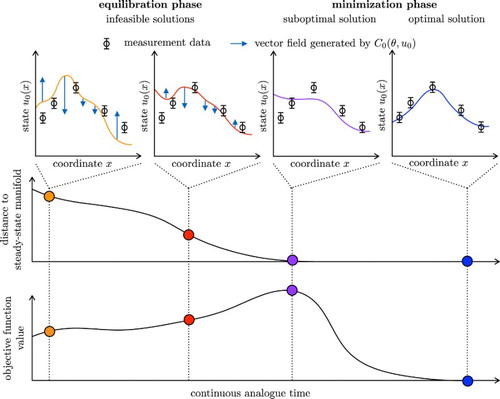
as illustrated in Figure .
Figure 1. The state of the system is illustrated along the trajectory of (Equation17(17)
(17) ). In the first phase, the equilibration phase, the system converges to the manifold. The solution is not feasible during this phase as the equality constraint,
, is violated. In the course of the equilibration, the objective function value might increase. In the second phase, the minimization phase, the objective function is minimized along the steady-state manifold.
4.2. Elliptic and parabolic PDE constraints
The continuous analogue for descent with elliptic PDE constraints can be generalized to problems with parabolic and elliptic PDE constraints. One possibility for doing so is to consider the partially reduced problem
(18)
(18) in which
denotes the solution to
with
. Given this formulation, we can use continuous analogue (Equation17
(17)
(17) ) with
(19)
(19) To avoid the need for the solution operator
, alternatively, a continuous analogue of the full problem can also be formulated. This is beyond the scope of this study, though, and will be subject of future research.
5. Local stability and convergence to a local optimum
The behaviour of the coupled ODE–PDE system (Equation17(17)
(17) ) introduced in the previous section depends on the properties of the objective function and the PDE model, as well as the retraction factor λ. To prove that a solution of (Equation17
(17)
(17) ) with an appropriate retraction factor λ is well defined and converges to the local minimizer
of (Equation5
(5)
(5) ), we impose the following assumptions.
Assumption 5.1
The descent direction vanishes at the minimizer of the optimization problem
Assumption 5.2
There exists such that for all
the following holds.
The operator
The operator
Assumption 5.3
The function is locally uniformly monotonically decreasing, i.e. there exist
and
such that
for all
and
.
Assumption 5.4
The sensitivity is locally Lipschitz continuous with respect to
i.e. there exists
such that
for all
and
.
Assumption 5.5
The mapping is uniformly monotonically decreasing on
i.e. there exists
such that
for all
.
Assumption 5.6
The descent direction g is locally Lipschitz continuous with respect to i.e. there exists
such that
for all
and
.
Moreover, g is uniformly bounded on i.e there exists
such that
for all
.
5.1. Elliptic PDE constraints
Using Assumptions 5.1–5.6 and the existence of a weak solution (Assumption 2.1), we can prove the following theorem on stability and convergence for the continuous analogue of the descent method for elliptic PDE constraints.
Theorem 5.1
Let Assumptions 5.1–5.6 be satisfied. Then there exists a such that for all
solutions to (Equation17
(17)
(17) ) are well defined for all r>0 and the local
minimizer
of the optimization problem (Equation5
(5)
(5) ) is a locally exponentially stable steady state of the system (Equation17
(17)
(17) ).
Proof.
Define and
, with
and
, where
exists, because of Assumption 5.2. We further define a Lyapunov function
. To prove Theorem 5.1, we will show that the Lyapunov function decreases exponentially. The derivative along the trajectories is given by
First, we bound the first summand from above, using (Equation17
(17)
(17) ), and Assumptions 5.1, 5.5 and 5.6,
Second, we bound the second summand from above, using (Equation17
(17)
(17) ) and
, as well as the fact that by Assumption 5.3 we have (Equation9
(9)
(9) ),
With Assumptions 5.3, 5.4 and 5.6, we get
Hence, we can estimate the derivative of the Lyapunov function,
To show that
decays exponentially, we have to show that
for some a>0. Based on our estimates, proving Theorem 5.1 reduces to finding a>0 with
(20)
(20) We want this inequality to be valid without restrictions on
or
. Due to the last term, we can therefore only consider values of a that are smaller than
. Hence, (Equation20
(20)
(20) ) is equivalent to
Since the first term in the inequality is greater or equal to 0, we have to find a>0 such that
Multiplying with
, we obtain a quadratic inequality for a
The roots of the quadratic polynomial are given by
with discriminant
The discriminant is always positive, therefore,
are real roots. In the following, we will assume that
, which can be achieved by choosing λ such that
. This choice is justified as follows. As the square root,
, is always positive,
, i.e.
needs to hold to ensure
. Squaring both sides of the inequality
(21)
(21) yields
Taking
ensures
.
Therefore, a either fulfils with
or
, provided
. Hence, we distinguish the following three cases:
for the relation of ,
and
as illustrated in Figure .
Figure 2. The function is illustrated with the two roots
and
and the three different positions of
, as well as possible positions of a.

Case (1): is equivalent to
If the term
is negative, the inequality cannot be valid. The term
is non-negative if
. In this case, we can square the inequality and get a contradiction (
).
Case (2): is equivalent to
This leads to a contradiction with the same arguments as in case (1).
Case (3): is equivalent to
The left-hand side
is non-negative for all
. With squaring, we get
. On the other hand, if the term
is negative, that is
, we have
. This is true for all λ, because d>0. In total, we find
for all
. Analogously we get for
that
is fulfilled for all
. Hence, we know that
holds for all
and only case (3) is valid.
Altogether, we find that a lies in the interval provided
. In this case, it also holds that
with
, where
is the embedding constant.
Remark 5.1
To tune the choice of the retraction factor λ, we now consider the fact that the value of a determines the speed at which decreases, thus a convenient choice of the retraction factor
maximizes a to yield the fastest exponential decay. In our case, this means maximizing
with respect to λ. An elementary computation yields
with equality iff
, thus
is monotonically increasing (strictly, if
) and therefore
In case
, we have
. Distinguishing the two cases for the absolute value yields the maximal value
, attained at all
.
This shows that (unless ) the exponential decay is maximized by choosing
as large as possible. Nevertheless, in practice, λ should not be chosen too large in order to avoid stiffness of system (Equation17
(17)
(17) ).
Remark 5.2
The proof provides a lower bound for the retraction factor λ, namely . In specific applications, it might not always be possible to explicitly compute all involved constants. If this is the case, an alternative Lyapunov function can be used to derive a lower bound for λ. A possible candidate for this Lyapunov function is
(22)
(22) With this choice and analogous computations as above, different lower bounds involving different constants can be derived. The lower bound for the retraction factor can be estimated as
with
(23)
(23) and
(24)
(24) This bound depends on θ, the current parameter estimates during computation, and therefore requires a posteriori adaptation of the retraction factor. A practical implementation of such a retraction factor choice involves the evaluation of functionals of the residuals
,
as well as sensitivities
(which can be done approximately, on a coarser computational mesh, and using adjoint techniques) is subject of future work.
Remark 5.3
If the cost function is locally convex but not locally uniformly convex, the parameters are identifiable but not strictly identifiable [Citation19]. In this case, defined by (Equation14
(14)
(14) ) is not uniformly monotone, but just monotone, i.e. formally
. In this case, using a projection P on the orthogonal complement of the null space of
might facilitate the proof of convergence on this subspace. A possible Lyapunov function in this case is given by
. Denoting the smallest positive eigenvalue of
with
, we require that
for all
. Then a retraction factor λ should be chosen
, with
(25)
(25) and
(26)
(26) However, the null space of
depends on the unknown optimal parameter
and can in general not be assessed a priori, thus leaving this approach for further investigation.
Remark 5.4
Locality in Theorem 5.1 is only imposed in terms of the size of in Assumptions 5.2–5.6. As a matter of fact, Assumptions 5.2, 5.3, 5.4, 5.6 will typically hold for
values in a larger neighbourhood of the solution, possibly after imposing certain constraints on the parameter values such as nonnegativity, in order to ensure that the model defined by
is valid. Smallness of
will mainly be required in Assumption 5.5 to guarantee, together with Assumption 5.1, that the descent direction defined by g really points towards
.
To enlarge the convergence radius, globalization strategies for the solution of nonlinear equations or optimization problems can be employed. In particular, as the analysis in [Citation20,Citation21] indicates, the strategy of using a particular time-stepping algorithm together with an appropriate step size control in place of the continuous flow defined by (Equation17(17)
(17) ), might enable to get rid of the locality assumption in Theorem 5.1. Indeed, with
for the choice (Equation15
(15)
(15) ), method (Equation17
(17)
(17) ) can at least formally be cast into the framework of [Citation20, Equation (5.1)], see also the introduction of [Citation21] for the infinite dimensional setting relevant here. However, the detailed conditions from [Citation21] would still have to be verified for our special setting, which will be subject of future research.
5.2. Elliptic and parabolic PDE constraints
As we consider the partially reduced form of the optimization problem with elliptic and parabolic PDE constraints (Equation18(18)
(18) ), the results established for the elliptic problem can be easily transferred given the existence of a solution operator for the parabolic problem.
Theorem 5.2
Let Assumptions 2.1, 5.1–5.6 be satisfied with g replaced by according to (Equation19
(19)
(19) ). Then there exists a
such that for all
solutions to
(27)
(27) are well defined for all r>0 and the local minimizer
of the
optimization problem (Equation4
(4)
(4) ) is a locally exponentially stable steady state of the system (Equation27
(27)
(27) ).
With the setting introduced in the last paragraph of Section 4, the result directly follows from Theorem 5.1.
6. Discussion of the assumptions
In this section, we discuss Assumptions 5.1–5.6 in more detail. In particular, we provide sufficient conditions for these assumptions which show that the assumptions are rather weak and fulfilled by many application problems.
Remark 6.1
Assumption 5.1
For the choice (Equation14(14)
(14) ) of g, this condition is satisfied due to the identity
This remains valid more generally for descent directions defined by (Equation15
(15)
(15) ), such as
Newton-type methods.
Remark 6.2
Assumptions 5.2 and 5.3
Dynamical systems in engineering, physics and life sciences will typically exhibit locally exponentially stable steady-state solutions. This implies that these systems are locally uniformly monotone. This is especially true for the optimal parameters and thus (for smooth
) also in a neighbourhood of
. Hence, around the true parameters, Assumption 5.3 and thus also the monotonicity part of Assumption 5.2 is locally fulfilled for most real-world systems.
An additional consequence of uniform monotonicity, hemicontinuity and coercivity of according to Assumption 5.2 is uniform monotonicity, hemicontinuity and coercivity of its linearization and thus, by the Theorem of Browder and Minty, existence and boundedness of the inverse
, is assured, as will be used below.
Remark 6.3
Assumption 5.4
The Lipschitz continuity of S is satisfied for example if
provided that is continuously (Frèchet) differentiable. This can be seen as follows.
We want to show that for all
,
and
, where
is the ith component of
.
Using for
yields
With
, we can further estimate
The fact that the inverses
,
exist and are bounded follows from the regularity of
and a perturbation argument. Taking
and
, i=1,2 and using that by continuity of
in a neighbourhood of
and by possibly decreasing
,
, we get
for any
. Therewith the operator
exists and is bounded by
Using this bound and local Lipschitz continuity with respect to
of the derivatives
and
results in
and hence
with
, where
denotes the bound of the derivative w.r.t.
of the steady-state residual.
Remark 6.4
Assumption 5.5
If the descent direction g is defined by (Equation14(14)
(14) ), then, according to [Citation19], Assumption 5.5 is equivalent to practical identifiability, which implies local structural identifiability of the parameter vector θ. The same holds true for more general choices (Equation15
(15)
(15) ), such as Newton-type methods, under a uniform positivity condition on
.
If local structural identifiability cannot be guaranteed, one can still use regularization [Citation22], e.g. by adding a term with positive definite Γ and positive α to the cost function
in (Equation5
(5)
(5) ) for which (Equation17
(17)
(17) ) yields a minimizer
. Regularization theory, e.g. [Citation22], provides convergence of
to a parameter
that is consistent with the observations as
.
Remark 6.5
Assumption 5.6
As an example, we check Assumption 5.6 for the case of a gradient descent-based update of θ, i.e. g according to (Equation14(14)
(14) ). We find
Here,
is Lipschitz continuous according to Remark 6.3. Also boundedness of
is fulfilled under the assumptions made in Remark 6.3, namely that
and
are locally uniformly bounded.
(28)
(28) If J is differentiable and the derivatives
and
are locally Lipschitz continuous with respect to
with Lipschitz constants
and
, respectively, and
is uniformly bounded on
, we can conclude
with
.
The more general choice (Equation15(15)
(15) ) requires additionally Lipschitz continuity of
, which in case of Newton-type methods with (Equation16
(16)
(16) ) amounts to higher smoothness of J and
.
Thus we have shown the following proposition.
Proposition 6.1
Let Assumption 6.1 be satisfied. Then there exist such that on
, Assumptions 5.1–5.6 are fulfilled.
Assumption 6.1
J is continuously
7. Application
To illustrate the continuous analogue of the descent method, we use it to study CCL21 gradient formation in biological tissues. This process is highly relevant in immune response [Citation23,Citation24] and described by a reaction–diffusion equation [Citation25]. In the following, we outline the model, estimate its parameters using the approach proposed in this paper and analyse the results.
7.1. Model formulation
CCL21 gradients are necessary for the guidance of dendritic cells towards lymphatic vessels [Citation26]. They are formed by the combination of several biological processes. The chemokine CCL21 is produced in the lymphatic vessels, which cover a subset domain of the domain Ω of interest,
. The source term is defined via the function
The concentration of free CCL21 is denoted by u. Free CCL21 binds to a sugar whose concentration is denoted by s. The binding yields immobilized CCL21 whose concentration is denoted by c. The parameters
denote the binding and unbinding rates, the diffusion coefficient, the degradation rate and the production rate of CCL21 from the lymphatic vessels, respectively. A PDE model for the process has been developed in [Citation25] and is given by
(29)
(29) for
and
, with initial conditions
,
and no-flux boundary conditions
where ν is the outer normal on Ω. The parameter
denotes the initial sugar concentration.
As the formation of the gradient is apparently fast, we consider the steady state of (Equation29(29)
(29) ). By considering the PDE for the time evolution of s and c, we find that
and
with the scaled CCL21 concentration
. Using the additional reformulation
,
, the scaled steady-state concentration of CCL21,
, has to fulfil
and the boundary conditions
.
For the considered process, imaging data have been collected [Citation27]. These images provide information about the localization of the lymphatic vessels (encoded in Q) and the concentration of immobilized CCL21. As the measured intensity values are corrupted by background fluorescence and as the data are not normalized, we model the readout following [Citation25] as
where b denotes the intensity of the background fluorescence,
is a scaling constant and
is the domain of the pixel k. As the parameters are structurally non-identifiable, we reformulate the models in terms of
and
in the parameter estimation to one parameter and just consider
and
.
The optimization problem is then given by
(30)
(30) where
,
is the scale parameter of the log-normally distributed measurement error and
,
. The parameter vector θ is given by
, with
.
All parameters are assumed to be non-negative due to their biological meaning. The spaces V and for which we examine the problem are
. The operator
is given by
. For these spaces and operators, it can easily be checked that all assumptions for applying the method (Equation17
(17)
(17) ) are satisfied.
7.2. Numerical implementation
For the numerical simulation of the biological process, we employed a finite element discretization of the PDE model. The discretization was obtained using the MATLAB PDE toolbox and accounts for the stationary topology of the model (Figure A). The mesh consists of 2170 elements and the concentrations in these elements are the state variables of the discretization. For parameter optimization using the coupled ODE–PDE model (Equation17(17)
(17) ), the same mesh was employed and the states of the discretized PDE were coupled with the ODE for the parameters. This yields a model with 2170+5 equations. The simulation-based method for parameter estimation was implemented in MATLAB extending the routine published in [Citation16]. The numerical simulation was performed using the MATLAB ODE solver ode15s, an implicit scheme applicable to stiff problems. To accelerate the calculations, we implemented the Jacobian of the coupled ODE–PDE model. The simulation of the continuous analogue was terminated, if the gradient of the right-hand side became small, i.e.
. Furthermore, simulations were interrupted whenever the objective function value became complex, which can happen due to the log-transformation of the output.
Figure 3. (A) Geometry of a lymphoid vessel obtained from biological imaging data [Citation27]. (B) Simulated data of the CCL21 gradient generated by simulating model (Equation29(29)
(29) ).
![Figure 3. (A) Geometry of a lymphoid vessel obtained from biological imaging data [Citation27]. (B) Simulated data of the CCL21 gradient generated by simulating model (Equation29(29) ut−DΔu=αQ−k1us+k−1c−γu,s˙=−k1us+k−1c,c˙=k1us−k−1c,(29) ).](/cms/asset/298a948f-4bd9-4e43-8bf5-63209c7bde55/gipe_a_1494167_f0003_c.jpg)
7.3. Simulated data
To evaluate the convergence properties of the proposed algorithm for the models, we considered published simulated data for the ground truth (similar to [Citation28]). The geometry of lymphatic tissue was extracted from the available imaging data [Citation27] using the MATLAB PDE toolbox. On this geometry, the discretized PDE was simulated using biologically plausible parameter values (Table ). The simulated data for CCL21 gradient formation process were corrupted by noise to obtain a plausible scenario (Figure B).
Table 1. True parameters, estimated parameters and parameter ranges for the latin hypercube sampling for the CCL21 model.
7.4. Optimization
The objective function for most parameter estimation problems is non-convex and can be multimodal. For this reason, we employed multi-start local
optimization using the continuous analogue for which we have established local convergence in this paper. The starting points for the local
optimizations were sampled using a latin hypercube approach with lower and upper bounds provided in Table . We used a linear parametrization for the states and a log-parametrization for the parameters following previous evaluations for biochemical systems [Citation29]. We did not implement any bounds for values of parameter or states. The implementation of the multi-start local optimization is based upon the MATLAB toolbox PESTO [Citation30]. The implementation of the objective function and finite element schemes was adapted from [Citation25]. For the local optimization with the continuous analogue, we chose the negative gradient as descent direction.
As a reference, we performed also multi-start local optimization using a discrete iterative optimization method. We used the state-of-the-art optimizer fmincon.m with the starting points sampled for the continuous analogue and the interior point algorithm implemented in the MATLAB Optimization Toolbox. This interior point algorithm employs either a Newton step, where the Hessian is approximated by the Broyden–Fletcher–Goldfarb–Shanno (BFGS) algorithm, or a conjugate gradient step using a trust region [Citation31–33]. The optimizer was provided with the objective function, the nonlinear constraint, as well as the corresponding derivatives. We used the same parametrization as for the continuous analogue and additionally constrained parameter values for in the optimization by the same upper and lower bounds used for the sampling (Table ). The value of
at the nodes of the mesh for the finite element discretization was constrained using upper and lower bounds for the optimization to lie in
. A total of 2000 iterations and 4000 function evaluations was allowed.
7.5. Comparison of continuous analogue and discrete iterative procedure
We performed 100 local optimization runs with the continuous analogue for a retraction factor and a discrete iterative method (Figure A). Both methods found the same best parameter value (Table ) and achieved a good fit to the data. The assessment of the results revealed a good convergence of the continuous analogue. Almost
of the runs achieved an objective function value which was comparable with the best objective function value found across all runs (relative difference
). Overall, 96% of the runs finished successfully, meaning that either the optimization was stopped because the stopping criterion was fulfilled or the maximum number of iterations was reached, while 4% of the runs stopped prematurely.
Figure 4. Results of parameter estimation for CCL21 model. (A) Sorted objective function values for the multi-start optimization with continuous analogue () and discrete iterative procedure. Converged runs are indicated in blue. (B) CPU time needed per optimizer run for the optimization using the continuous analogue and the discrete iterative procedure (lighter grey colour indicates runs which stopped because the maximal number of iterations was reached). The box covers the range between the 25th and the 75th percentile of the distribution. The median CPU time is indicated by a line. (C) Histogram of values for
(Remark 5.2) obtained for 1000 points sampled in parameter-state space. (D) Percentage of completed runs (top), converged runs (middle)and median as well as 25th and 75th percentile of the runtime of completed runs (bottom) for different values of λ. For each value of λ, 100 local optimization runs were performed.
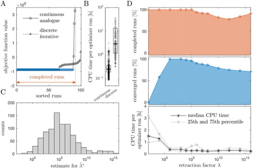
The discrete iterative optimization converged for of the runs to the optimal value (Figure A). Accordingly, the success rate was substantially lower than for the proposed continuous analogue. Of the runs which did not converge to the global optimum 25 runs were stopped because the maximal number of iterations was reached.
For the considered problem, the continuous analogue outperformed the discrete iterative method regarding the CPU time (Figure B). We found a median CPU time of 15 minutes for the continuous solver and 174 minutes for the discrete iterative procedure. In light of the fact that the discrete iterative method uses second-order information, it is interesting to observe that a continuous analogue using the negative gradient is more efficient. One possible explanation is that the efficiency of the continuous analogue is a result of the application of sophisticated numerical solvers. The adaptive, implicit solver ode15s, which is provided with the analytical Jacobian of the ODE–PDE model, might facilitate large step-sizes and fast convergence. Indeed, the Jacobian also provides second-order information.
7.6. Evaluation of retraction factor influence
As an analytical calculation of the bound for the retraction factor was not possible, we sampled 1000 points in parameter-state space and evaluated the estimate for the lower bound (Remark 5.2). The histogram of the resulting values for
is presented in Figure C. The values for
span many orders of magnitude, and the distribution peaks at
. This result indicated that for different starting points very different retraction factors might be ideal.
To investigate the convergence properties for the different values of the retraction factor λ, we performed 100 local optimization runs for a range of different retraction factors. For each retraction factor, we assessed the number of completed runs and the number of converged runs (Figure D). Interestingly, as λ was increased the percentage of completed runs decreased. Yet, for large retraction factors many of the completed runs also converged, while for small retraction factors no runs converged as the maximum number of iterations becomes too large. The median CPU time for the optimization of one run decreased for increasing values of λ (Figure D). Notably, for the small values, the median CPU time was nearly six to seven times higher than the smallest one. The quantiles indicate that also the variability was higher for small values of λ. These results indicated that the retraction factor should be chosen large enough but not too large.
In summary, the analysis of the model of CCL21 gradient formation revealed that the retraction factor λ has a substantial influence on the convergence properties as well as the run time. For low values of λ starts did not converge while for large values of λ increasing stiffness of the problem could be observed. In an intermediate regime, which could here also be found by random sampling, we found the best convergence properties.
8. Conclusion and outlook
Parameter estimation is an important problem in a wide range of applications. Robustness and performance of the available iterative methods is, however, often limited. In this study, we introduced continuous analogues of descent methods for optimization with PDE constraints. For these continuous analogues, we proved local convergence of their solutions to the optima. The necessary assumptions are fulfilled for a wide range of application problems, rendering the results interesting for several research fields.
We demonstrated the applicability of continuous analogues for a model of gradient formation in biological tissues and compared them with an iterative discrete procedure. The results highlight the potential of the continuous analogues, e.g. a high convergence rate and lower computation times than the discrete iterative procedure. For the comparison, we used the MATLAB optimization routine fmincon.m, a state-of-the-art discrete iterative procedure. Alternatives would be IPOPT or KNITRO. As fmincon is a generic interior point method, there might apparently be approaches which are efficient for the considered PDE-constrained problems (see also the no free lunch theorem [Citation34]). The evaluation of the influence of the retraction factor revealed the importance of an appropriate choice of the retraction factor as well as the issue of premature stopping. In this study, we provide a lower bound for λ which ensures local convergence. As this bound might, however, be conservative and can only be assessed pointwise, the use of adaptive methods might be interesting. To address the issue of premature stopping, bounds for parameters and state variables have to be implemented, e.g. by including log-barrier functions [Citation35] in the objective function or through projection into the feasible space.
In the application problem, we only considered elliptic PDE constraints as for the proposed continuous analogues parabolic constraints can be encapsulated in the objective function. This changes the objective function landscape and indirectly influences the convergence. Conceptually, it should also be possible to formulate continuous analogues which do not require a solution operator for the parabolic PDE but also have the solution of the parabolic PDE as a state variable. This mathematically more elegant approach is left for future research.
In conclusion, this study presented continuous analogues for a new problem class. Similar to other problem classes for which continuous analogues have been established [Citation15,Citation16], we expect an improvement of convergence and computation time. The continuous analogues for optimization also complement recent work on simulation-based methods for uncertainty analysis [Citation36]. The efficient implementation of these methods in easily accessible software packages should be a focus of future research as it would render the methods available to a broad community.
The method and its analysis apply as they are to the case of infinite dimensional parameters θ. However, in that situation, the inverse problem of identifying θ is often ill-posed, so the assumption of practical identifiability (cf. Assumption 5.5 and Remark 6.4) might not be satisfied. To restore stability, regularization can be employed, as pointed out in Remark 6.4.
Future research in this context will be concerned with globalization strategies, such as those proposed in [Citation20,Citation21], cf. Remark 5.4.
Disclosure statement
No potential conflict of interest was reported by the authors.
Additional information
Funding
References
- Isakov V. Inverse problems for partial differential equations. 2nd ed. New York, NY: Springer; 2006. (Applied Mathematical Sciences; 127).
- Tarantola A. Inverse problem theory and methods for model parameter estimation. Philadelphia: SIAM Society for Industrial and Applied Mathematics; 2005.
- Banks H, Kunisch K. Estimation techniques for distributed parameter systems. Boston, Basel, Berlin: Birkhäuser; 1989. (Systems & Control: Foundations & Applications; 1).
- Bock H, Carraro T, Jäeger W, et al. Model based parameter estimation: theory and applications. Berlin, Heidelberg: Springer; 2013. (Contributions in Mathematical and Computational Sciences; 4).
- Carvalho EP, Martínez J, Martínez JM, et al. On optimization strategies for parameter estimation in models governed by partial differential equations. Math Comput Simul. 2015;114:14–24. doi: 10.1016/j.matcom.2010.07.020
- Hinze M, Pinnau R, Ulbrich M, et al. Optimization with PDE constraints. Netherlands: Springer; 2009. (Mathematical Modelling: Theory and Applications; 23).
- Ito K, Kunisch K. Lagrange multiplier approach to variational problems and applications. Philadelphia: SIAM Society for Industrial and Applied Mathematics; 2008. (Advances in Design and Control; 15).
- Xun X, Cao J, Mallick B, et al. Parameter estimation of partial differential equation models. J Am Stat Assoc. 2013;108:1009–1020. doi: 10.1080/01621459.2013.794730
- Nielsen BF, Lysaker M, Grøttum P. Computing ischemic regions in the heart with the bidomain model – first steps towards validation. IEEE Trans Med Imaging. 2013 Jun;32(6):1085–1096. doi: 10.1109/TMI.2013.2254123
- Airapetyan RG, Ramm AG, Smirnova AB. Continuous methods for solving nonlinear ill-posed problems. Operator Theory Appl. 2000;25:111.
- Kaltenbacher B, Neubauer A, Ramm AG. Convergence rates of the continuous regularized Gauss-Newton method. J Inv Ill-Posed Problems. 2002;10:261–280. doi: 10.1515/jiip.2002.10.3.261
- Tanabe K. Continuous Newton–Raphson method for solving and underdetermined system of nonlinear equations. Nonlinear Anal Theory Methods Appl. 1979;3(4):495–503. doi: 10.1016/0362-546X(79)90064-6
- Tanabe K. A geometric method in nonlinear programming. J Optim Theory Appl. 1980;30(2):181–210. doi: 10.1007/BF00934495
- Watson L, Bartholomew-Biggs M, Ford J. Optimization and nonlinear equations. Journal of computational and applied mathematics. Vol. 124. Amsterdam: The Netherlands; 2001.
- Tanabe K. Global analysis of continuous analogues of the Levenberg–Marquardt and Newton–Raphson methods for solving nonlinear equations. Ann Inst Statist Math. 1985;37(Part B):189–203. doi: 10.1007/BF02481091
- Fiedler A, Raeth S, Theis FJ, et al. Tailored parameter optimization methods for ordinary differential equation models with steady-state constraints. BMC Syst Biol. 2016 Aug;10:80.
- Rosenblatt M, Timmer J, Kaschek D. Customized steady-state constraints for parameter estimation in non-linear ordinary differential equation models. Front Cell Dev Biol. 2016;4:41. doi: 10.3389/fcell.2016.00041
- Zeidler E. Nonlinear functional analysis and its applications II/B: nonlinear monotone operators. New York, NY: Springer; 1990.
- Faller D, Klingmüller U, Timmer J. Simulation methods for optimal experimental design in systems biology. Simulation. 2003;79(12):717–725. doi: 10.1177/0037549703040937
- Potschka A. Backward step control for global Newton-type methods. SIAM J Numer Anal. 2016;54(1):361–387. doi: 10.1137/140968586
- Potschka A. Backward step control for Hilbert space problems. 2017; ArXiv:1608.01863 [math.NA].
- Engl H, Hanke M, Neubauer A. Regularization of inverse problems. Dordrecht: Kluwer Academic Publishers; 2000. (Mathematics and Its Applications; 375).
- Alvarez D, Vollmann EH, von Andrian UH. Mechanisms and consequences of dendritic cell migration. Immunity. 2008;29(3):325–342. 2017/05/19. doi: 10.1016/j.immuni.2008.08.006
- Mellman I, Steinman RM. Dendritic cells. Cell. 2001;106(3):255–258. 2017/05/19. doi: 10.1016/S0092-8674(01)00449-4
- Hock S, Hasenauer J, Theis FJ. Modeling of 2D diffusion processes based on microscopy data: parameter estimation and practical identifiability analysis. BMC Bioinformatics. 2013;14(10):1–6.
- Schumann K, Lammermann T, Bruckner M, et al. Immobilized chemokine fields and soluble chemokine gradients cooperatively shape migration patterns of dendritic cells. Immunity. 2010 May;32(5):703–713. doi: 10.1016/j.immuni.2010.04.017
- Weber M, Hauschild R, Schwarz J, et al. Interstitial dendritic cell guidance by haptotactic chemokine gradients. Science. 2013;339:328–332. doi: 10.1126/science.1228456
- Hross S Parameter estimation and uncertainty quantification for reaction-diffusion models in image based systems biology [dissertation]. München: Technische Universität München; 2016.
- Raue A, Schilling M, Bachmann J, et al. Lessons learned from quantitative dynamical modeling in systems biology. PLoS One. 2013 Sep;8(9):e74335. doi: 10.1371/journal.pone.0074335
- Stapor P, Weindl D, Ballnus B, et al. Pesto: parameter estimation toolbox. Bioinformatics. 2017 Oct;btx676–btx676. Available from: http://dx.doi.org/10.1093/bioinformatics/btx676.
- Byrd RH, Hribar ME, Nocedal J. An interior point algorithm for large-scale nonlinear programming. SIAM J Optim. 1999;9:877–900. doi: 10.1137/S1052623497325107
- Byrd RH, Gilbert JC, Nocedal J. A trust region method based on interior point techniques for nonlinear programming. Math Program. 2000 Nov;89(1):149–185. Available from: http://dx.doi.org/10.1007/PL00011391.
- Waltz RA, Morales JL, Nocedal J, et al. An interior algorithm for nonlinear optimization that combines line search and trust region steps. Math Program. 2006 Jul;107(3):391–408. Available from: http://dx.doi.org/10.1007/s10107-004-0560-5.
- Wolpert DH, Macready WG. No free lunch theorems for optimization. IEEE Trans Evol Comput. 1997 Apr;1(1):67–82. doi: 10.1109/4235.585893
- Boyd S, Vandenberghe L. Convex optimisation. UK: Cambridge University Press; 2004.
- Boiger R, Hasenauer J, Hross S, et al. Integration based profile likelihood calculation for PDE constrained parameter estimation problems. Inverse Prob. 2016 Dec;32(12):125009. doi: 10.1088/0266-5611/32/12/125009