A class of multistep numerical difference schemes applied in inverse heat conduction problem with a control parameter

ABSTRACT

As this paper is concerned with a class of multistep numerical difference techniques to solve one-dimensional parabolic inverse problems with source control parameter $p\left(t\right)$, we apply the linear multistep method combining with Lagrange interpolation to develop three different numerical difference schemes. The problem of numerical differentiation with noisy scattered data is mildly ill-posed, the smoothing spline model based on Tikhonov regularization method is developed to compute numerical derivative contaminated by noise error. Simultaneously, the truncation error estimations and the convergence conclusions are proposed for the above difference methods respectively. The results of numerical tests with different noise levels are given to show that the presented algorithms are accurate and effective.

KEYWORDS:

• Inverse heat conduction problem
• Tikhonov regularization method
• numerical difference schemes
• linear multistep method
• Lagrange interpolation

2010 MSC CLASSIFICATIONS:

• 65N21
• 65L06
• 65D05

1. Introduction

Inverse heat conduction problems (IHCPs) arise in many fields of physics such as control modelling with heat propagation, mechanics, heat flux, the remote sensing technology, signal processing and industrial controlling. Many researchers have been attracted to study this field because their theories possess distinct novelty and are applicable to a broad range of applications.

It is known that heat conduction process is very smooth, but the studies of IHCPs are more difficult for its irreversible. The IHCP is ill-posed in some sense that any small errors for measured values on some specified points can result in a large error to the solution [1], which implies that the resultant discretized matrix is ill-conditioned, i.e. that the solution is potentially sensitive to perturbations. So the key is to find a stable algorithm to overcome the ill-posedness of problems, using a reasonable regularization method generally [2,3]. Furthermore, Tikhonov regularization method plays an important role in efficiently solving the ill-posed problems [4].

Many numerical algorithms for solving one-dimensional IHCP have been proposed during the last decade, including the finite difference method (FDM) [5–10], the radial basis function (RBF) method [11–15], the method of fundamental solutions (MFS) [1,16,17], the collocation method (CM) [18] and the boundary element method (BEM) used in the determination of a spacewise-dependent heat source [19], etc. Meanwhile, some numerical technologies are applied in multidimensional parabolic equations [20–23], Dehghan et al. [24–31] proposed the meshless method of RBFs to solve a series of nonlinear high dimensional partial differential equations, and applied other schemes to solve inverse parabolic problems to obtain effective results. We consider that the main advantage of the forward FDM, whose form is simple and easy to compute. Moreover, when we handle the one-dimensional inverse parabolic equations, it is different between the spatial domain and temporal domain in the physical view [14]. For an aspect of constructing tools with high accuracy, we apply the linear multistep technology to develop more accurate difference schemes. In practical problems, the overspecification node $x^{\ast }$ cannot just be chosen a mesh point $x_i$, so we use cubic or quartic Lagrange polynomial interpolation method to approximate function $\tilde{u}(x^{\ast },t)$.

This paper is organized as follows. In Section 2, we present a class of IHCP with a source control parameter $p\left(t\right)$ and introduce the main idea of transforming it into a direct problem to solve. In Section 3, first we describe the process of constructing numerical finite difference schemes by using linear multistep technologies. Second, we give three different FDMs. Furthermore, we deduce the order results of truncation error and the convergence estimates, including the case of $E\left(t\right)$ with noise. The numerical results for the test used are given in Section 4. Finally we summarize this paper in Section 5.

2. Problem statement

We now consider a class of IHCP with the source control parameter $p\left(t\right)$, which is stated as follows: (1) $\frac{\mathrm{\partial }w}{\mathrm{\partial }t}=\frac{{\mathrm{\partial }}^{2}w}{\mathrm{\partial }{x}^2}+p\left(t\right)w+\varphi (x,t),0<x<1,0<t\le T,$(1) with the initial condition (2) $w(x,0)=f\left(x\right),0\le x\le 1,$(2) the boundary conditions (3) $w(0,t)=g_0\left(t\right),0\le t\le T,$(3) (4) $w(1,t)=g_1\left(t\right),0\le t\le T,$(4) and the overspecification at a node $x^{\ast }\in (0,1)$ in the spatial domain (5) $w(x^{\ast },t)=E\left(t\right),0\le t\le T,$(5) where $\varphi (x,t),f\left(x\right),g_0\left(t\right),g_1\left(t\right)$ and $E\left(t\right)\left(E\right(t)\ne 0)$ are the given functions, but the functions $w(x,t)$ and $p\left(t\right)$ are unknown. The function $w(x,t)$ denotes temperature distribution which is the exact solution to the IHCP, and $p\left(t\right)$ is a source control parameter, where (5(5) $w(x^{\ast },t)=E\left(t\right),0\le t\le T,$(5) ) produces a desired temperature at each time t and a given point $x^{\ast }$ in the spatial domain. The system of equations (1(1) $\frac{\mathrm{\partial }w}{\mathrm{\partial }t}=\frac{{\mathrm{\partial }}^{2}w}{\mathrm{\partial }{x}^2}+p\left(t\right)w+\varphi (x,t),0<x<1,0<t\le T,$(1) )–(5(5) $w(x^{\ast },t)=E\left(t\right),0\le t\le T,$(5) ) represents a heat transfer process, and the existence, uniqueness of the solution and some applications of this problem are introduced in [32–35]. The aim of solving the problem is to identify the function $w(x,t)$ and the parameter $p\left(t\right)$. Since the formula (1(1) $\frac{\mathrm{\partial }w}{\mathrm{\partial }t}=\frac{{\mathrm{\partial }}^{2}w}{\mathrm{\partial }{x}^2}+p\left(t\right)w+\varphi (x,t),0<x<1,0<t\le T,$(1) ) includes two unknown functions $w(x,t)$ and $p\left(t\right)$, so we adopt the following treatment by J.R. Cannon [33,36], which can transform Equations (1(1) $\frac{\mathrm{\partial }w}{\mathrm{\partial }t}=\frac{{\mathrm{\partial }}^{2}w}{\mathrm{\partial }{x}^2}+p\left(t\right)w+\varphi (x,t),0<x<1,0<t\le T,$(1) )–(4(4) $w(1,t)=g_1\left(t\right),0\le t\le T,$(4) ) into another direct parabolic problem.

Let (6) $r\left(t\right)=e^{-{\int }_0^{t}p\left(s\right)\mathrm{d}s}$(6) and (7) $u(x,t)=r\left(t\right)w(x,t),$(7) which can eliminate the nonlinear term $p\left(t\right)w$ from Equation (1(1) $\frac{\mathrm{\partial }w}{\mathrm{\partial }t}=\frac{{\mathrm{\partial }}^{2}w}{\mathrm{\partial }{x}^2}+p\left(t\right)w+\varphi (x,t),0<x<1,0<t\le T,$(1) ) and to obtain a nonlocal parabolic equation, then the problems (1(1) $\frac{\mathrm{\partial }w}{\mathrm{\partial }t}=\frac{{\mathrm{\partial }}^{2}w}{\mathrm{\partial }{x}^2}+p\left(t\right)w+\varphi (x,t),0<x<1,0<t\le T,$(1) )–(4(4) $w(1,t)=g_1\left(t\right),0\le t\le T,$(4) ) can be transformed into the following equations: (8) $\frac{\mathrm{\partial }u}{\mathrm{\partial }t}=\frac{{\mathrm{\partial }}^{2}u}{\mathrm{\partial }{x}^2}+r\left(t\right)\varphi (x,t),0<x<1,0<t\le T,$(8) with the initial condition (9) $u(x,0)=f\left(x\right),0\le x\le 1,$(9) and the boundary conditions (10) $u(0,t)=r\left(t\right)g_0\left(t\right),0\le t\le T,$(10) (11) $u(1,t)=r\left(t\right)g_1\left(t\right),0\le t\le T.$(11) By (5(5) $w(x^{\ast },t)=E\left(t\right),0\le t\le T,$(5) ) and (7(7) $u(x,t)=r\left(t\right)w(x,t),$(7) ), $r\left(t\right)$ can be obtained by (12) $r\left(t\right)=\frac{u(x^{\ast },t)}{E\left(t\right)},$(12) and $w(x,t)$ can be presented by (13) $w(x,t)=\frac{u(x,t)}{r\left(t\right)},$(13) then we can obtain the control parameter $p\left(t\right)$ as (14) $p\left(t\right)=-\frac{r^{\prime }\left(t\right)}{r\left(t\right)},$(14) where the superscript ${}^{\prime }$ represents the first derivative of some function in this paper. In addition, the general algorithms of this paper consisting of two subproblems are as follows:

$\mathbf{A}\mathbf{1}$. First, we compute the numerical solutions $\tilde{u}(x_i,t_j)$ (or ${\tilde{u}}^{\delta }(x_i,t_j)$) of $u(x_i,t_j)$ by multistep difference technologies and use Lagrange polynomial interpolation to compute $\tilde{u}(x^{\ast },t_j)$ (or ${\tilde{u}}^{\delta }(x^{\ast },t_j)$), further to obtain $\tilde{r}\left(t_j\right)$ (or ${\tilde{r}}^{\delta }\left(t_j\right)$) by (12(12) $r\left(t\right)=\frac{u(x^{\ast },t)}{E\left(t\right)},$(12) ), then get $\tilde{w}(x_i,t_j)$ (or ${\tilde{w}}^{\delta }(x_i,t_j)$) by (13(13) $w(x,t)=\frac{u(x,t)}{r\left(t\right)},$(13) ).

$\mathbf{A}\mathbf{2}$. For a set of given scattered data $\left\{\tilde{r}\right(t_j){\}}_{j=1}^n$ (or $\left\{{\tilde{r}}^{\delta }\right(t_j){\}}_{j=1}^n$) above, we use the numerical differential scheme combining with Tikhonov regularization method to obtain the smooth regularized solution ${\tilde{r}}_{\alpha }\left(t\right)$ (or ${\tilde{r}}_{\alpha }^{\delta }\left(t\right)$), further to compute ${\tilde{p}}_{\alpha }\left(t_j\right)=-\left(\right({\tilde{r}}_{\alpha }^{\prime }\left(t_j\right)\left)/\right(\tilde{r}\left(t_j\right)\left)\right)$ (or ${\tilde{p}}_{\alpha }^{\delta }\left(t_j\right)=-\left(\right(\left({\tilde{r}}_{\alpha }^{\delta }{)}^{\prime }\right(t_j)\left)/\right({\tilde{r}}^{\delta }\left(t_j\right)\left)\right)$) by (14(14) $p\left(t\right)=-\frac{r^{\prime }\left(t\right)}{r\left(t\right)},$(14) ).

Remark 2.1

If the data in (1(1) $\frac{\mathrm{\partial }w}{\mathrm{\partial }t}=\frac{{\mathrm{\partial }}^{2}w}{\mathrm{\partial }{x}^2}+p\left(t\right)w+\varphi (x,t),0<x<1,0<t\le T,$(1) )–(5(5) $w(x^{\ast },t)=E\left(t\right),0\le t\le T,$(5) ) are smooth and compatible, then the problem (1(1) $\frac{\mathrm{\partial }w}{\mathrm{\partial }t}=\frac{{\mathrm{\partial }}^{2}w}{\mathrm{\partial }{x}^2}+p\left(t\right)w+\varphi (x,t),0<x<1,0<t\le T,$(1) )–(5(5) $w(x^{\ast },t)=E\left(t\right),0\le t\le T,$(5) ) is equivalent to the problem (8(8) $\frac{\mathrm{\partial }u}{\mathrm{\partial }t}=\frac{{\mathrm{\partial }}^{2}u}{\mathrm{\partial }{x}^2}+r\left(t\right)\varphi (x,t),0<x<1,0<t\le T,$(8) )–(12(12) $r\left(t\right)=\frac{u(x^{\ast },t)}{E\left(t\right)},$(12) ), and the solution of this parabolic problem exists uniquely, which is smooth from the standard regularization theory of parabolic equations. In addition, if $u(x,t)$ is obtained numerically, the functions $w(x,t)$ and $p\left(t\right)$ can be computed by the forms (13(13) $w(x,t)=\frac{u(x,t)}{r\left(t\right)},$(13) ) and (14(14) $p\left(t\right)=-\frac{r^{\prime }\left(t\right)}{r\left(t\right)},$(14) ) respectively, it means that the problem (1(1) $\frac{\mathrm{\partial }w}{\mathrm{\partial }t}=\frac{{\mathrm{\partial }}^{2}w}{\mathrm{\partial }{x}^2}+p\left(t\right)w+\varphi (x,t),0<x<1,0<t\le T,$(1) )–(5(5) $w(x^{\ast },t)=E\left(t\right),0\le t\le T,$(5) ) is mildly ill-posed in [8,33,37,38].

Remark 2.2

When the measured data $E\left(t\right)$ is exact in Section 3.1.3, the problem $\mathbf{A}\mathbf{1}$ above is well posed by Theorem 3.3. However, the problem $\mathbf{A}\mathbf{2}$ above is ill-posed by Theorem 3.4, in this case, the regularization parameter ${\alpha }_1$ depends on the errors from $\mathbf{A}\mathbf{1}$ with respect to the step sizes τ and h, i.e. if ${\alpha }_1=\tau +h^2$, the convergence can be obtained as $\tau ,h\to 0$.

Remark 2.3

In Section 3.1.4, when $E\left(t\right)$ has noise of level δ, i.e. $|E^{\delta }\left(t\right)-E\left(t\right)|\le \delta$ for all $t\in [0,T]$, then the problems $\mathbf{A}\mathbf{1}$ and $\mathbf{A}\mathbf{2}$ above are both ill-posed. As shown in Theorem 3.6, the step sizes τ and h should be selected according to δ in order to obtain the order of convergence ${\delta }^{1/2}$ for ${\tilde{w}}^{\delta }(x_i,t_j)$ in $\mathbf{A}\mathbf{1}$. Furthermore, as shown in Theorem 3.8, the step sizes τ, h, and the regularization parameter ${\alpha }_1^{\delta }$ are related to δ in $\mathbf{A}\mathbf{2}$, i.e. if $\tau ={\delta }^{1/2}$ and ${\alpha }_1^{\delta }={\delta }^{1/2}$, the order of convergence is ${\delta }^{\left(\nu -1\right)/4\nu }$, $\nu \ge 2$.

3. Multistep numerical difference schemes

We divide the domain $[0,1]\times [0,T]$ into an $M\times N$ uniform mesh with the spatial step-size $h=1/M$ in the x direction and the temporal step-size $\tau =T/N$, where M and N are positive integers. Let $\mathrm{\Omega }=\left\{\right(x_i,t_j),x_i=ih,t_j=j\tau ,i=0,1,\dots ,M,j=0,1,\dots ,N\}$. We assume $\tilde{u}(x_i,t_j)$ is an approximation value of $u(x_i,t_j)$, the values $\tilde{w}(x_i,t_j),\tilde{r}\left(t_j\right)$ and $\tilde{p}\left(t_j\right)$ are the similar approximations of $w(x_i,t_j),r\left(t_j\right)$ and $p\left(t_j\right)$ respectively.

On the left side of Equation (8(8) $\frac{\mathrm{\partial }u}{\mathrm{\partial }t}=\frac{{\mathrm{\partial }}^{2}u}{\mathrm{\partial }{x}^2}+r\left(t\right)\varphi (x,t),0<x<1,0<t\le T,$(8) ), $\mathrm{\partial }u/\mathrm{\partial }t$ can be substituted by (15) $\frac{\mathrm{\partial }u(x_i,t_j)}{\mathrm{\partial }t}\approx \frac{u(x_i,t_{j+1})-u(x_i,t_j)}{\tau }$(15) at the grid point $(x_i,t_j)$, where $i=0,1,\dots ,M,j=0,1,\dots ,N-1$. The formula ${\mathrm{\partial }}^{2}u/\mathrm{\partial }{x}^2$ on the right side of Equation (8(8) $\frac{\mathrm{\partial }u}{\mathrm{\partial }t}=\frac{{\mathrm{\partial }}^{2}u}{\mathrm{\partial }{x}^2}+r\left(t\right)\varphi (x,t),0<x<1,0<t\le T,$(8) ) can be approximated by the linear multistep methods [39], the key is to construct a k-step linear discretization equation as follows: (16) $\sum _{i=0}^k{a}_i\frac{{\mathrm{\partial }}^{2}u(x_{n+i},t_j)}{\mathrm{\partial }{x}^2}\approx \frac{1}{h^2}\sum _{i=0}^k{b}_{i}u(x_{n+i},t_j),$(16) where $n=0,1,\dots ,M-k,j=0,1,\dots ,N$, $a_i$ and $b_i$ are real constants. In order to determine the parameters $a_i$ and $b_i$, we first define the following operator: (17) $L\left[u\right(x,t);h]=\sum _{i=0}^k\left[b_{i}u(x+ih,t)-h^2{a}_i\frac{{\mathrm{\partial }}^{2}u(x+ih,t)}{\mathrm{\partial }{x}^2}\right],$(17) and expand $u(x+ih,t)$ and $\left({\mathrm{\partial }}^{2}u(x+ih,t)\right)/\mathrm{\partial }{x}^2$ at point x by Taylor polynomials, then we can find (18) $L\left[u\right(x,t);h]=C_{0}u(x,t)+C_{1}h\frac{\mathrm{\partial }u(x,t)}{\mathrm{\partial }x}+C_2{h}^2\frac{{\mathrm{\partial }}^{2}u(x,t)}{\mathrm{\partial }{x}^2}+\cdots +C_q{h}^q\frac{{\mathrm{\partial }}^{q}u(x,t)}{\mathrm{\partial }{x}^q}+\cdots ,$(18) where $C_0,C_1,\dots ,C_q$ are constants and satisfy (19) $\begin{array}{rl}{C}_0& =\sum _{i=0}^k{b}_i,\\ C_1& =\sum _{i=0}^{k}i{b}_i,\\ C_2& =\frac{1}{2!}\sum _{i=0}^k{i}^2{b}_i-\sum _{i=0}^k{a}_i,\\ & \cdots \\ C_q& =\frac{1}{q!}\sum _{i=0}^k{i}^q{b}_i-\frac{1}{(q-2)!}\sum _{i=0}^k{i}^{q-2}{a}_i,q=3,4,\dots ,\end{array}$(19) by choosing suitable values k, $a_i$ and $b_i$ such that $C_0=C_1=\cdots =C_q=0$, and $C_{q+1}\ne 0$, so we get the following truncation error: (20) $L\left[u\right(x,t);h]=C_{q+1}{h}^{q+1}\frac{{\mathrm{\partial }}^{q+1}u(x,t)}{\mathrm{\partial }{x}^{q+1}}+O\left(h^{q+2}\right).$(20) By substituting $u(x+ih,t)$ and $\left({\mathrm{\partial }}^{2}u(x+ih,t)\right)/\mathrm{\partial }{x}^2$ in Equation (17(17) $L\left[u\right(x,t);h]=\sum _{i=0}^k\left[b_{i}u(x+ih,t)-h^2{a}_i\frac{{\mathrm{\partial }}^{2}u(x+ih,t)}{\mathrm{\partial }{x}^2}\right],$(17) ) for $u(x_{n+i},t_j)$ and $\left({\mathrm{\partial }}^{2}u(x_{n+i},t_j)\right)/\mathrm{\partial }{x}^2$, and we can obtain the k-step discrete equation  (16(16) $\sum _{i=0}^k{a}_i\frac{{\mathrm{\partial }}^{2}u(x_{n+i},t_j)}{\mathrm{\partial }{x}^2}\approx \frac{1}{h^2}\sum _{i=0}^k{b}_{i}u(x_{n+i},t_j),$(16) ) with its local truncated error $C_{q+1}{h}^{q+1}\left(\right({\mathrm{\partial }}^{q+1}u(x_{n+i},t_j)\left)/\right(\mathrm{\partial }{x}^{q+1}\left)\right)+O\left(h^{q+2}\right)$.

3.1. Three-point numerical difference scheme

3.1.1. Algorithm 1

Let $k=2,j=1,2,\dots ,N$, in Equations (15(15) $\frac{\mathrm{\partial }u(x_i,t_j)}{\mathrm{\partial }t}\approx \frac{u(x_i,t_{j+1})-u(x_i,t_j)}{\tau }$(15) )–(16(16) $\sum _{i=0}^k{a}_i\frac{{\mathrm{\partial }}^{2}u(x_{n+i},t_j)}{\mathrm{\partial }{x}^2}\approx \frac{1}{h^2}\sum _{i=0}^k{b}_{i}u(x_{n+i},t_j),$(16) ), and denote the grid ratio $\rho =\tau /h^2$. We choose an appropriate coefficient set $\{a_0,a_1,a_2\}$, correspondingly obtain the derived set $\{b_0,b_1,b_2\}$ and the nodes-subscript set $\{i_0,i_1,i_2\}$ in Table 1, so we can get the general difference equation formula: (21) $\begin{array}{rl}\tilde{u}(x_i,t_j)=& \tilde{u}(x_i,t_{j-1})+\rho \left\{b_0\tilde{u}\right(x_{i_0},t_{j-1})+b_1\tilde{u}(x_{i_1},t_{j-1})\\ & +b_2\tilde{u}(x_{i_2},t_{j-1})\}+\tau \tilde{r}(t_{j-1}\left)\varphi \right(x_i,t_{j-1}).\end{array}$(21)

Table 1. The different configuration parameters in formula (21(21) $\begin{array}{rl}\tilde{u}(x_i,t_j)=& \tilde{u}(x_i,t_{j-1})+\rho \left\{b_0\tilde{u}\right(x_{i_0},t_{j-1})+b_1\tilde{u}(x_{i_1},t_{j-1})\\ & +b_2\tilde{u}(x_{i_2},t_{j-1})\}+\tau \tilde{r}(t_{j-1}\left)\varphi \right(x_i,t_{j-1}).\end{array}$(21) ).

i	$a_0$	$a_1$	$a_2$	$b_0$	$b_1$	$b_2$	$i_0$	$i_1$	$i_2$
0	1	0	0	1	$-2$	1	0	1	2
$1\le i\le M-1$	0	1	0	1	$-2$	1	i−1	i	i+1
M	0	0	1	1	$-2$	1	M−2	M−1	M

Note that $\tilde{r}\left(t_0\right)=1$ and $\tilde{u}(x_i,0)=f\left(x_i\right),0\le i\le M$ by (6(6) $r\left(t\right)=e^{-{\int }_0^{t}p\left(s\right)\mathrm{d}s}$(6) ) and (9(9) $u(x,0)=f\left(x\right),0\le x\le 1,$(9) ), respectively. In practice, the overspecification node $x^{\ast }$ cannot just be chosen as a mesh point $x_i,i=0,1,\dots ,M$, so we use cubic-Lagrange polynomial interpolation method to compute $\tilde{u}(x^{\ast },t_j)$, whose structure is simple, and to achieve the required accuracy of proposed methods. According to the location of $x^{\ast }$, there are three cases to be proposed as follows:

$1)$ If $x^{\ast }\in (x_0,x_1)$, then $\tilde{u}(x^{\ast },t_j)$ yields (22) $\tilde{u}(x^{\ast },t_j)=\sum _{k=1}^4\tilde{u}(x_k,t_j)L_{3,k}\left(x^{\ast }\right),1\le j\le N.$(22) $2)$ If $x^{\ast }\in [x_i,x_{i+3}]$, $1\le i\le M-4$, then $\tilde{u}(x^{\ast },t_j)$ yields (23) $\tilde{u}(x^{\ast },t_j)=\sum _{k=i}^{i+3}\tilde{u}(x_k,t_j)L_{3,k}\left(x^{\ast }\right),1\le j\le N.$(23) $3)$ If $x^{\ast }\in (x_{M-1},x_M)$, then $\tilde{u}(x^{\ast },t_j)$ yields (24) $\tilde{u}(x^{\ast },t_j)=\sum _{k=M-4}^{M-1}\tilde{u}(x_k,t_j)L_{3,k}\left(x^{\ast }\right),1\le j\le N,$(24) the above $L_{3,k}\left(x\right)$ denotes a cubic-Lagrange basis function, and (25) $L_{3,k}\left(x\right)=\frac{{\omega }_4\left(x\right)}{(x-x_k){\omega }_4^{\mathrm{\prime }}\left(x_k\right)},$(25) where ${\omega }_4\left(x\right)=\prod _{k=i}^{i+3}(x-x_k)$, $x_k$ indicates an interpolation node in the domain $[x_1,x_{M-1}]$. Then according to the formula (12(12) $r\left(t\right)=\frac{u(x^{\ast },t)}{E\left(t\right)},$(12) ), the approximation of $r\left(t_j\right)$ can be obtained by (26) $\tilde{r}\left(t_j\right)=\frac{\tilde{u}(x^{\ast },t_j)}{E\left(t_j\right)},1\le j\le N,$(26) the boundary values $\tilde{u}(x_0,t_j)$ and $\tilde{u}(x_M,t_j)$ will be updated by Equations (10(10) $u(0,t)=r\left(t\right)g_0\left(t\right),0\le t\le T,$(10) ) and (11(11) $u(1,t)=r\left(t\right)g_1\left(t\right),0\le t\le T.$(11) ) as follows: (28) $\tilde{u}(x_0,t_j)=\tilde{r}\left(t_j\right)g_0\left(t_j\right)=\frac{g_0\left(t_j\right)}{E\left(t_j\right)}\tilde{u}(x^{\ast },t_j),$(28) (29) $\tilde{u}(x_M,t_j)=\tilde{r}\left(t_j\right)g_1\left(t_j\right)=\frac{g_1\left(t_j\right)}{E\left(t_j\right)}\tilde{u}(x^{\ast },t_j),$(29) where $1\le j\le N$. According to the formula (13(13) $w(x,t)=\frac{u(x,t)}{r\left(t\right)},$(13) ), the approximation solution to $w(x_i,t_j)$ can be computed by (29) $\tilde{w}(x_i,t_j)=\frac{\tilde{u}(x_i,t_j)}{\tilde{r}\left(t_j\right)},0\le i\le M,0\le j\le N.$(29)

3.1.2. Algorithm 2

Since the values $\tilde{r}\left(t_j\right)$ in Equation (26(26) $\tilde{r}\left(t_j\right)=\frac{\tilde{u}(x^{\ast },t_j)}{E\left(t_j\right)},1\le j\le N,$(26) ) can only be derived by the discrete measured data with errors, we must apply the numerical differential technique to get the corresponding discrete data for the values $\tilde{p}\left(t_j\right)$ by Equation (14(14) $p\left(t\right)=-\frac{r^{\prime }\left(t\right)}{r\left(t\right)},$(14) ). However, the problem of numerical differentiation is well known to be ill-posed, it means that any small errors for the measurement values on some specified points can cause large errors to the implemented derivative [40–43]. Thus it is the key aim to develop a stable scheme to deal with the ill-posed problem. The traditional FDM is simple and effective for precise data, but it is failed to compute accurate derivative of the measured values with noisy data, since the size of mesh depends on the noise level, i.e. which should not be too small, in other words, the number of measured points should not be chosen too big, otherwise, it may be very large for the final errors of the approximation solutions [41,44].

Recently, some numerical differential schemes based on the Tikhonov regularization technique and the smoothing spline have been proposed [40–42,44,45], based on a suitable strategy of the regularization parameter, these differential methods with regularization are effective and stable. In this paper, we use numerical differentiation with regularization method presented in [41,42] to compute the values ${\tilde{r}}^{\prime }\left(t_j\right)$.

For given a set of measured values $\{{\tilde{r}}_j{\}}_{j=1}^n$ with the error data, and define $X_{\nu }=\{r\mid r\in C^{\nu -1}(\mathbb{R}),r^{\left(\nu \right)}\in L^2(\mathbb{R}\left)\right\}$. Consider a smoothing functional on $X_{\nu }$: (30) ${\mathrm{{\rm Y}}}_{\nu }\left(r\right)=\frac{1}{n}\sum _{j=1}^n{\left(r\left(t_j\right)-{\tilde{r}}_j\right)}^2+{\alpha }_1\parallel r^{\left(\nu \right)}{\parallel }_{L^2\left(\mathbb{R}\right)}^2,$(30) where $\nu \ge 2$ is a fixed integer, $n\ge \nu$, let $\{t_j{\}}_1^n$ be a set of distinct points on $[a,b]$, and ${\alpha }_1$ is a regularization parameter under Tikhonov regularization sense.

Lemma 3.1

[41]

Define (31) ${\tilde{r}}_{{\alpha }_1}\left(t\right)=\sum _{j=1}^n{\overline{p}}_j|t-t_j{|}^{2\nu -1}+\sum _{j=1}^{\nu }{\overline{q}}_j{t}^{j-1},$(31) where coefficients $\{{\overline{p}}_j{\}}_1^n$ and $\{{\overline{q}}_j{\}}_1^{\nu }$ satisfy (32) ${\tilde{r}}_{{\alpha }_1}\left(t_j\right)+2(2\nu -1)!(-1{)}^{\nu }{\alpha }_{1}n{\overline{p}}_j={\tilde{r}}_j,j=1,2,\dots ,n,$(32) (33) $\sum _{j=1}^n{\overline{p}}_j{t}_j^i=0,i=0,1,\dots ,\nu -1,$(33) then ${\tilde{r}}_{{\alpha }_1}$ is a unique minimizer of the smoothing functional (30(30) ${\mathrm{{\rm Y}}}_{\nu }\left(r\right)=\frac{1}{n}\sum _{j=1}^n{\left(r\left(t_j\right)-{\tilde{r}}_j\right)}^2+{\alpha }_1\parallel r^{\left(\nu \right)}{\parallel }_{L^2\left(\mathbb{R}\right)}^2,$(30) ), i.e. ${\mathrm{{\rm Y}}}_{\nu }\left({\tilde{r}}_{{\alpha }_1}\right)=\underset{r\in X_{\nu }}{min}{\mathrm{{\rm Y}}}_{\nu }\left(r\right)\le {\mathrm{{\rm Y}}}_{\nu }\left(y\right)$, $\mathrm{\forall }y\in X_{\nu }$.

Lemma 3.2

[41]

There is a unique solution for linear system of Equations (32(32) ${\tilde{r}}_{{\alpha }_1}\left(t_j\right)+2(2\nu -1)!(-1{)}^{\nu }{\alpha }_{1}n{\overline{p}}_j={\tilde{r}}_j,j=1,2,\dots ,n,$(32) ) and (33(33) $\sum _{j=1}^n{\overline{p}}_j{t}_j^i=0,i=0,1,\dots ,\nu -1,$(33) ).

By differentiating ${\tilde{r}}_{{\alpha }_1}\left(t\right)$ of (31(31) ${\tilde{r}}_{{\alpha }_1}\left(t\right)=\sum _{j=1}^n{\overline{p}}_j|t-t_j{|}^{2\nu -1}+\sum _{j=1}^{\nu }{\overline{q}}_j{t}^{j-1},$(31) ) with respect to t, then we have (34) ${\tilde{r}}_{{\alpha }_1}^{\prime }\left(t\right)=(2\nu -1)\sum _{j=1}^n{\overline{p}}_j\mathrm{sign}(t-t_j)|t-t_j{|}^{2\nu -2}+\sum _{j=1}^{\nu }(j-1){\overline{q}}_j{t}^{j-2}.$(34) Furthermore, the approximation values ${\tilde{p}}_{{\alpha }_1}\left(t_j\right)$ of $p\left(t_j\right)$ can be obtained by (14(14) $p\left(t\right)=-\frac{r^{\prime }\left(t\right)}{r\left(t\right)},$(14) ) (35) ${\tilde{p}}_{{\alpha }_1}\left(t_j\right)=-\frac{{\tilde{r}}_{{\alpha }_1}^{\prime }\left(t_j\right)}{\tilde{r}\left(t_j\right)},0\le j\le N.$(35) For convenience, the above approach is called 3PNDS in this paper.

3.1.3. The convergence estimates of 3PNDS for $E\left(t\right)$ without noise

The proof of the convergence estimate for 3PNDS consists of the following details. In order to express convenience and simplicity, we define (36) ${\mathrm{\Delta }}_h^2{\tilde{u}}_i^j=\left(\tilde{u}(x_{i+1},t_j)+\tilde{u}(x_{i-1},t_j)-2\tilde{u}(x_i,t_j)\right)/h^2,$(36) and assume that $G_0^j=g_0\left(t_j\right)/E\left(t_j\right)$, $G_M^j=g_1\left(t_j\right)/E\left(t_j\right)$, ${\mathrm{\Phi }}_i^j=\varphi (x_i,t_j)/E\left(t_j\right)$, combining with Equations (9(9) $u(x,0)=f\left(x\right),0\le x\le 1,$(9) )–(12(12) $r\left(t\right)=\frac{u(x^{\ast },t)}{E\left(t\right)},$(12) ), (21(21) $\begin{array}{rl}\tilde{u}(x_i,t_j)=& \tilde{u}(x_i,t_{j-1})+\rho \left\{b_0\tilde{u}\right(x_{i_0},t_{j-1})+b_1\tilde{u}(x_{i_1},t_{j-1})\\ & +b_2\tilde{u}(x_{i_2},t_{j-1})\}+\tau \tilde{r}(t_{j-1}\left)\varphi \right(x_i,t_{j-1}).\end{array}$(21) )–(28(29) $\tilde{u}(x_M,t_j)=\tilde{r}\left(t_j\right)g_1\left(t_j\right)=\frac{g_1\left(t_j\right)}{E\left(t_j\right)}\tilde{u}(x^{\ast },t_j),$(29) ) and (36(36) ${\mathrm{\Delta }}_h^2{\tilde{u}}_i^j=\left(\tilde{u}(x_{i+1},t_j)+\tilde{u}(x_{i-1},t_j)-2\tilde{u}(x_i,t_j)\right)/h^2,$(36) ), then we have two corresponding systems for j=1 and $j\ge 2$ respectively as follows: (37) $\begin{array}{rl}\left(\tilde{u}\right(x_0,t_1)-\tilde{u}(x_0,t_0\left)\right)/\tau & ={\mathrm{\Delta }}_h^2{\tilde{u}}_1^0+\varphi (x_0,t_0),\\ \left(\tilde{u}\right(x_i,t_1)-\tilde{u}(x_i,t_0\left)\right)/\tau & ={\mathrm{\Delta }}_h^2{\tilde{u}}_i^0+\varphi (x_i,t_0),1\le i\le M-1,\\ \left(\tilde{u}\right(x_M,t_1)-\tilde{u}(x_M,t_0\left)\right)/\tau & ={\mathrm{\Delta }}_h^2{\tilde{u}}_{M-1}^0+\varphi (x_M,t_0),\\ \tilde{u}(x_i,0)& =f\left(x_i\right),0\le i\le M,\\ \tilde{u}(x_i,t_1)& =G_i^1\tilde{u}(x^{\ast },t_1),i=0\mathrm{or}M\left(\mathrm{update}\mathrm{boundary}\right),\end{array}$(37) and (38) $\begin{array}{rl}\left(\tilde{u}\right(x_0,t_j)-\tilde{u}(x_0,t_{j-1}\left)\right)/\tau & ={\mathrm{\Delta }}_h^2{\tilde{u}}_1^{j-1}+{\mathrm{\Phi }}_0^{j-1}\tilde{u}(x^{\ast },t_{j-1}),j\ge 2,\\ \left(\tilde{u}\right(x_i,t_j)-\tilde{u}(x_i,t_{j-1}\left)\right)/\tau & ={\mathrm{\Delta }}_h^2{\tilde{u}}_i^{j-1}+{\mathrm{\Phi }}_i^{j-1}\tilde{u}(x^{\ast },t_{j-1}),1\le i\le M-1,j\ge 2,\\ \left(\tilde{u}\right(x_M,t_j)-\tilde{u}(x_M,t_{j-1}\left)\right)/\tau & ={\mathrm{\Delta }}_h^2{\tilde{u}}_{M-1}^{j-1}+{\mathrm{\Phi }}_M^{j-1}\tilde{u}(x^{\ast },t_{j-1}),j\ge 2,\\ \tilde{u}(x_i,0)& =f\left(x_i\right),0\le i\le M,\\ \tilde{u}(x_i,t_j)& =G_i^j\tilde{u}(x^{\ast },t_j),i=0\mathrm{or}M,j\ge 2\left(\mathrm{update}\mathrm{boundary}\right).\end{array}$(38) Suppose that $e_i^j=u(x_i,t_j)-\tilde{u}(x_i,t_j)$, $e_{\ast }^j=u(x^{\ast },t_j)-\tilde{u}(x^{\ast },t_j)$, according to Taylor's expansion, $e_i^j$ and $e_{\ast }^j$ satisfy the following formulas by Equations (37(37) $\begin{array}{rl}\left(\tilde{u}\right(x_0,t_1)-\tilde{u}(x_0,t_0\left)\right)/\tau & ={\mathrm{\Delta }}_h^2{\tilde{u}}_1^0+\varphi (x_0,t_0),\\ \left(\tilde{u}\right(x_i,t_1)-\tilde{u}(x_i,t_0\left)\right)/\tau & ={\mathrm{\Delta }}_h^2{\tilde{u}}_i^0+\varphi (x_i,t_0),1\le i\le M-1,\\ \left(\tilde{u}\right(x_M,t_1)-\tilde{u}(x_M,t_0\left)\right)/\tau & ={\mathrm{\Delta }}_h^2{\tilde{u}}_{M-1}^0+\varphi (x_M,t_0),\\ \tilde{u}(x_i,0)& =f\left(x_i\right),0\le i\le M,\\ \tilde{u}(x_i,t_1)& =G_i^1\tilde{u}(x^{\ast },t_1),i=0\mathrm{or}M\left(\mathrm{update}\mathrm{boundary}\right),\end{array}$(37) ) and (38(38) $\begin{array}{rl}\left(\tilde{u}\right(x_0,t_j)-\tilde{u}(x_0,t_{j-1}\left)\right)/\tau & ={\mathrm{\Delta }}_h^2{\tilde{u}}_1^{j-1}+{\mathrm{\Phi }}_0^{j-1}\tilde{u}(x^{\ast },t_{j-1}),j\ge 2,\\ \left(\tilde{u}\right(x_i,t_j)-\tilde{u}(x_i,t_{j-1}\left)\right)/\tau & ={\mathrm{\Delta }}_h^2{\tilde{u}}_i^{j-1}+{\mathrm{\Phi }}_i^{j-1}\tilde{u}(x^{\ast },t_{j-1}),1\le i\le M-1,j\ge 2,\\ \left(\tilde{u}\right(x_M,t_j)-\tilde{u}(x_M,t_{j-1}\left)\right)/\tau & ={\mathrm{\Delta }}_h^2{\tilde{u}}_{M-1}^{j-1}+{\mathrm{\Phi }}_M^{j-1}\tilde{u}(x^{\ast },t_{j-1}),j\ge 2,\\ \tilde{u}(x_i,0)& =f\left(x_i\right),0\le i\le M,\\ \tilde{u}(x_i,t_j)& =G_i^j\tilde{u}(x^{\ast },t_j),i=0\mathrm{or}M,j\ge 2\left(\mathrm{update}\mathrm{boundary}\right).\end{array}$(38) ) (39) $\begin{array}{rl}(e_0^1-e_0^0)/\tau & ={\mathrm{\Delta }}_h^2{e}_1^0+{\widetilde{ϵ}}_0^0,\\ (e_i^1-e_i^0)/\tau & ={\mathrm{\Delta }}_h^2{e}_i^0+{\widetilde{ϵ}}_i^0,1\le i\le M-1,\\ (e_M^1-e_M^0)/\tau & ={\mathrm{\Delta }}_h^2{e}_{M-1}^0+{\widetilde{ϵ}}_M^0,\\ e_i^0& =0,0\le i\le M,\\ e_i^1& =G_i^1{e}_{\ast }^1,i=0\mathrm{or}M,\end{array}$(39) and (40) $\begin{array}{rl}(e_0^j-e_0^{j-1})/\tau & ={\mathrm{\Delta }}_h^2{e}_1^{j-1}+{\mathrm{\Phi }}_0^{j-1}{e}_{\ast }^{j-1}+{ϵ}_0^{j-1},j\ge 2,\\ (e_i^j-e_i^{j-1})/\tau & ={\mathrm{\Delta }}_h^2{e}_i^{j-1}+{\mathrm{\Phi }}_i^{j-1}{e}_{\ast }^{j-1}+{ϵ}_i^{j-1},1\le i\le M-1,j\ge 2,\\ (e_M^j-e_M^{j-1})/\tau & ={\mathrm{\Delta }}_h^2{e}_{M-1}^{j-1}+{\mathrm{\Phi }}_M^{j-1}{e}_{\ast }^{j-1}+{ϵ}_M^{j-1},j\ge 2,\\ e_i^0& =0,0\le i\le M,\\ e_i^j& =G_i^j{e}_{\ast }^j,i=0\mathrm{or}M,j\ge 2,\end{array}$(40) where ${\widetilde{ϵ}}_0^0$, ${\widetilde{ϵ}}_i^0$, ${\widetilde{ϵ}}_M^0$, ${ϵ}_0^{j-1}$, ${ϵ}_i^{j-1}$ and ${ϵ}_M^{j-1}$ are the truncation errors derived by the discretization of differential equation. In addition, if the given functions $g_0\left(t\right)$, $g_1\left(t\right)$, $E\left(t\right)$ ($E\left(t\right)\ne 0$) and $\varphi (x,t)$ are continuous on the interval $[0,T]$ or $[0,1]\times [0,T]$, then the discretization values $\left\{{\mathrm{\Phi }}_i^j\right\}$ and $\left\{G_i^j\right\}$ are bounded, so there exists a positive constant K such that the following inequalities hold: $\underset{0\le i\le M,1\le j\le N-1}{max}|{\mathrm{\Phi }}_i^j|\le K,\underset{i=0\mathrm{or}M,1\le j\le N}{max}|G_i^j|\le K.$ The error bound of Lagrange polynomial is developed as follows:

Lemma 3.3

[46]

Let $x_0,x_1,\dots ,x_n$ be distinct numbers in the interval $[a,b]$ and $P\left(x\right)\in C^{n+1}[a,b]$, and define ${\omega }_{n+1}\left(x\right)=(x-x_0)(x-x_1)\dots (x-x_n)$. Then, there exists a number $\xi \left(x\right)\in (a,b)$ (generally unknown) between $x_0,x_1,\dots ,x_n$, and satisfying the following formula: $\begin{array}{r}\mathrm{\%}P\left(x\right)=L_n\left(x\right)+\frac{P^{(n+1)}\left(\xi \right(x\left)\right)}{(n+1)!}{\omega }_{n+1}\left(x\right),\end{array}$ where $L_n\left(x\right)$ is Lagrange interpolating polynomial of degree n given by $\begin{array}{rl}\mathrm{\%}{L}_n\left(x\right)& =P\left(x_0\right)L_{n,0}\left(x\right)+\cdots +P\left(x_n\right)L_{n,n}\left(x\right)\\ & =\sum _{k=0}^{n}P\left(x_k\right)L_{n,k}\left(x\right),\end{array}$ where $L_{n,k}\left(x\right)=\left({\omega }_{n+1}\left(x\right)\right)/\left((x-x_k){\omega }_{n+1}^{\mathrm{\prime }}\left(x_k\right)\right)$.

Theorem 3.1

Let $u(x,t)\in C^{4,2}\left(\right[0,1]\times [0,T\left]\right)$, $\varphi (x,t)\in C[0,1]\times [0,T]$, $f\left(x\right)\in C[0,1]$, $g_0\left(t\right)\in C[0,T]$, $g_1\left(t\right)\in C[0,T]$, $E\left(t\right)\in C[0,T]$ $\left(E\right(t)\ne 0)$, then the truncation error order of 3PNDS can reach $O(\tau +h)$ at least.

Proof.

If the given point $x^{\ast }\in [x_{s-1},x_{s+2}]$, where $1\le s\le M-2$, then we can obtain the following conclusion by Lemma 3.3: (41) $\begin{array}{rl}u(x,t)& =\sum _{k=s-1}^{s+2}u(x_k,t)L_{3,k}\left(x\right)\\ & +O\left(\right(x-x_{s-1}\left)\right(x-x_s\left)\right(x-x_{s+1}\left)\right(x-x_{s+2}\left)\right),\end{array}$(41) furthermore, x and t in Equation (41(41) $\begin{array}{rl}u(x,t)& =\sum _{k=s-1}^{s+2}u(x_k,t)L_{3,k}\left(x\right)\\ & +O\left(\right(x-x_{s-1}\left)\right(x-x_s\left)\right(x-x_{s+1}\left)\right(x-x_{s+2}\left)\right),\end{array}$(41) ) are replaced by $x^{\ast }$ and $t_j$, respectively, we have (42) $\begin{array}{rl}u(x^{\ast },t_j)& =\sum _{k=s-1}^{s+2}u(x_k,t_j)L_{3,k}\left(x^{\ast }\right)\\ & +O\left(\right(x^{\ast }-x_{s-1}\left)\right(x^{\ast }-x_s\left)\right(x^{\ast }-x_{s+1}\left)\right(x^{\ast }-x_{s+2}\left)\right),\\ & =\sum _{k=s-1}^{s+2}u(x_k,t_j)L_{3,k}\left(x^{\ast }\right)+O\left(h^4\right),\end{array}$(42) where $j=1,2,\dots ,N$. We define the following linear operators: (43) $\tilde{L}u(x,t)=\frac{\mathrm{\partial }u(x,t)}{\mathrm{\partial }t}-\frac{{\mathrm{\partial }}^{2}u(x,t)}{\mathrm{\partial }{x}^2}-\frac{\varphi (x,t)}{E\left(t\right)}u(x^{\ast },t)$(43) and (44) $\begin{array}{rl}{\tilde{L}}_{h}u(x,t)& =\frac{u(x,t+\tau )-u(x,t)}{\tau }-\frac{u(x+h,t)+u(x-h,t)-2u(x,t)}{h^2}\\ & -\frac{\varphi (x,t)}{E\left(t\right)}\sum _{k=s-1}^{s+2}u(x_k,t)L_{3,k}\left(x^{\ast }\right),\end{array}$(44) (45) $\begin{array}{rl}{\tilde{L}}_{0}u(x,t)& =\frac{u(x,t+\tau )-u(x,t)}{\tau }-\frac{u(x+2h,t)+u(x,t)-2u(x+h,t)}{h^2}\\ & -\frac{\varphi (x,t)}{E\left(t\right)}\sum _{k=s-1}^{s+2}u(x_k,t)L_{3,k}\left(x^{\ast }\right),\end{array}$(45) (46) $\begin{array}{rl}{\tilde{L}}_{M}u(x,t)& =\frac{u(x,t+\tau )-u(x,t)}{\tau }-\frac{u(x,t)+u(x-2h,t)-2u(x-h,t)}{h^2}\\ & -\frac{\varphi (x,t)}{E\left(t\right)}\sum _{k=s-1}^{s+2}u(x_k,t)L_{3,k}\left(x^{\ast }\right).\end{array}$(46) Now we replace x and t in Equations (43(43) $\tilde{L}u(x,t)=\frac{\mathrm{\partial }u(x,t)}{\mathrm{\partial }t}-\frac{{\mathrm{\partial }}^{2}u(x,t)}{\mathrm{\partial }{x}^2}-\frac{\varphi (x,t)}{E\left(t\right)}u(x^{\ast },t)$(43) )–(46(46) $\begin{array}{rl}{\tilde{L}}_{M}u(x,t)& =\frac{u(x,t+\tau )-u(x,t)}{\tau }-\frac{u(x,t)+u(x-2h,t)-2u(x-h,t)}{h^2}\\ & -\frac{\varphi (x,t)}{E\left(t\right)}\sum _{k=s-1}^{s+2}u(x_k,t)L_{3,k}\left(x^{\ast }\right).\end{array}$(46) ) with $x_i$ and $t_j$, respectively. In addition, we define the following truncation error operators $T_h$, $T_0$ and $T_M$ on $u(x_i,t_j)$, here the truncation errors derive from two parts, i.e. one is caused by the truncation of infinite Taylor series, the other comes from the truncation of Lagrange interpolation, then we have (47) $T_{h}u(x_i,t_j)={\tilde{L}}_{h}u(x_i,t_j)-\tilde{L}u(x_i,t_j),$(47) (48) $T_{0}u(x_i,t_j)={\tilde{L}}_{0}u(x_i,t_j)-\tilde{L}u(x_i,t_j),$(48) (49) $T_{M}u(x_i,t_j)={\tilde{L}}_{M}u(x_i,t_j)-\tilde{L}u(x_i,t_j).$(49) ♯ When j=0, since $r\left(t_0\right)=1$ in Equation (6(6) $r\left(t\right)=e^{-{\int }_0^{t}p\left(s\right)\mathrm{d}s}$(6) ). By the forms (15(15) $\frac{\mathrm{\partial }u(x_i,t_j)}{\mathrm{\partial }t}\approx \frac{u(x_i,t_{j+1})-u(x_i,t_j)}{\tau }$(15) )–(20(20) $L\left[u\right(x,t);h]=C_{q+1}{h}^{q+1}\frac{{\mathrm{\partial }}^{q+1}u(x,t)}{\mathrm{\partial }{x}^{q+1}}+O\left(h^{q+2}\right).$(20) ) and (43(43) $\tilde{L}u(x,t)=\frac{\mathrm{\partial }u(x,t)}{\mathrm{\partial }t}-\frac{{\mathrm{\partial }}^{2}u(x,t)}{\mathrm{\partial }{x}^2}-\frac{\varphi (x,t)}{E\left(t\right)}u(x^{\ast },t)$(43) )–(46(46) $\begin{array}{rl}{\tilde{L}}_{M}u(x,t)& =\frac{u(x,t+\tau )-u(x,t)}{\tau }-\frac{u(x,t)+u(x-2h,t)-2u(x-h,t)}{h^2}\\ & -\frac{\varphi (x,t)}{E\left(t\right)}\sum _{k=s-1}^{s+2}u(x_k,t)L_{3,k}\left(x^{\ast }\right).\end{array}$(46) ), combining with Taylor's expansion, we have (50) $\tilde{L}u(x,t)=\frac{\mathrm{\partial }u(x,t)}{\mathrm{\partial }t}-\frac{{\mathrm{\partial }}^{2}u(x,t)}{\mathrm{\partial }{x}^2}-\varphi (x,t)$(50) and (51) $\begin{array}{rl}{\tilde{L}}_{h}u(x,t)& =\frac{u(x,t+\tau )-u(x,t)}{\tau }-\frac{u(x+h,t)+u(x-h,t)-2u(x,t)}{h^2}\\ & -\varphi (x,t),\end{array}$(51) (52) $\begin{array}{rl}{\tilde{L}}_{0}u(x,t)& =\frac{u(x,t+\tau )-u(x,t)}{\tau }-\frac{u(x+2h,t)+u(x,t)-2u(x+h,t)}{h^2}\\ & -\varphi (x,t),\end{array}$(52) (53) $\begin{array}{rl}{\tilde{L}}_{M}u(x,t)& =\frac{u(x,t+\tau )-u(x,t)}{\tau }-\frac{u(x,t)+u(x-2h,t)-2u(x-h,t)}{h^2}\\ & -\varphi (x,t).\end{array}$(53) By the formulas (47(47) $T_{h}u(x_i,t_j)={\tilde{L}}_{h}u(x_i,t_j)-\tilde{L}u(x_i,t_j),$(47) )–(49(49) $T_{M}u(x_i,t_j)={\tilde{L}}_{M}u(x_i,t_j)-\tilde{L}u(x_i,t_j).$(49) ) and (50(50) $\tilde{L}u(x,t)=\frac{\mathrm{\partial }u(x,t)}{\mathrm{\partial }t}-\frac{{\mathrm{\partial }}^{2}u(x,t)}{\mathrm{\partial }{x}^2}-\varphi (x,t)$(50) )–(53(53) $\begin{array}{rl}{\tilde{L}}_{M}u(x,t)& =\frac{u(x,t+\tau )-u(x,t)}{\tau }-\frac{u(x,t)+u(x-2h,t)-2u(x-h,t)}{h^2}\\ & -\varphi (x,t).\end{array}$(53) ), we can obtain the truncation error orders as follows: (54) $T_{h}u(x_i,t_j)=O(\tau +h^2),1\le i\le M-1,$(54) (55) $T_{0}u(x_i,t_j)=O(\tau +h),i=0,$(55) (56) $T_{M}u(x_i,t_j)=O(\tau +h),i=M,$(56) from the above deduction, the forms (54(54) $T_{h}u(x_i,t_j)=O(\tau +h^2),1\le i\le M-1,$(54) )–(56(56) $T_{M}u(x_i,t_j)=O(\tau +h),i=M,$(56) ) show that the truncation error order of 3PNDS can reach $O(\tau +h)$ at least for j=0.

♯ When $1\le j\le N-1$, let $T_{\ast }$ be the truncation error operator on $u(x^{\ast },t)$, then we have the following truncation error estimation of $u(x^{\ast },t_j)$ by Equation (42(42) $\begin{array}{rl}u(x^{\ast },t_j)& =\sum _{k=s-1}^{s+2}u(x_k,t_j)L_{3,k}\left(x^{\ast }\right)\\ & +O\left(\right(x^{\ast }-x_{s-1}\left)\right(x^{\ast }-x_s\left)\right(x^{\ast }-x_{s+1}\left)\right(x^{\ast }-x_{s+2}\left)\right),\\ & =\sum _{k=s-1}^{s+2}u(x_k,t_j)L_{3,k}\left(x^{\ast }\right)+O\left(h^4\right),\end{array}$(42) ): (57) $\begin{array}{rl}{T}_{\ast }u(x^{\ast },t_j)& =u(x^{\ast },t_j)-\sum _{k=s-1}^{s+2}u(x_k,t_j)L_{3,k}\left(x^{\ast }\right)\\ & =O\left(h^4\right),1\le j\le N.\end{array}$(57) According to the forms (42(42) $\begin{array}{rl}u(x^{\ast },t_j)& =\sum _{k=s-1}^{s+2}u(x_k,t_j)L_{3,k}\left(x^{\ast }\right)\\ & +O\left(\right(x^{\ast }-x_{s-1}\left)\right(x^{\ast }-x_s\left)\right(x^{\ast }-x_{s+1}\left)\right(x^{\ast }-x_{s+2}\left)\right),\\ & =\sum _{k=s-1}^{s+2}u(x_k,t_j)L_{3,k}\left(x^{\ast }\right)+O\left(h^4\right),\end{array}$(42) )–(46(46) $\begin{array}{rl}{\tilde{L}}_{M}u(x,t)& =\frac{u(x,t+\tau )-u(x,t)}{\tau }-\frac{u(x,t)+u(x-2h,t)-2u(x-h,t)}{h^2}\\ & -\frac{\varphi (x,t)}{E\left(t\right)}\sum _{k=s-1}^{s+2}u(x_k,t)L_{3,k}\left(x^{\ast }\right).\end{array}$(46) ) and (47(47) $T_{h}u(x_i,t_j)={\tilde{L}}_{h}u(x_i,t_j)-\tilde{L}u(x_i,t_j),$(47) )–(49(49) $T_{M}u(x_i,t_j)={\tilde{L}}_{M}u(x_i,t_j)-\tilde{L}u(x_i,t_j).$(49) ), we can obtain the following conclusions: (58) $T_{h}u(x_i,t_j)=O(\tau +h^2),1\le i\le M-1,$(58) (59) $T_{0}u(x_i,t_j)=O(\tau +h),i=0,$(59) (60) $T_{M}u(x_i,t_j)=O(\tau +h),i=M,$(60) where $j=0,1,\dots ,N-1$. In short, by the results (54(54) $T_{h}u(x_i,t_j)=O(\tau +h^2),1\le i\le M-1,$(54) )–(56(56) $T_{M}u(x_i,t_j)=O(\tau +h),i=M,$(56) ) and (58(58) $T_{h}u(x_i,t_j)=O(\tau +h^2),1\le i\le M-1,$(58) )–(60(60) $T_{M}u(x_i,t_j)=O(\tau +h),i=M,$(60) ), the truncation error order of 3PDNS can reach $O(\tau +h)$ at least. According to the above arguments, the truncation error order is independent of the distribution interval of $x^{\ast }$.

The estimates of the truncation errors ${\widetilde{ϵ}}_i^0$ and ${ϵ}_i^j$ are as follows:

Lemma 3.4

Suppose that $u(x,t)\in C^{4,2}\left(\right[0,1]\times [0,T\left]\right)$, $\varphi (x,t)\in C[0,1]\times [0,T]$, $f\left(x\right)\in C[0,T]$, $g_0\left(t\right)\in C[0,T]$, $g_1\left(t\right)\in C[0,T]$, $E\left(t\right)\in C[0,T]$ and $E\left(t\right)\ne 0$, then there exists a positive constant ${\tilde{Q}}_1$ such that $\begin{array}{rl}\underset{1\le i\le M-1}{max}|{\widetilde{ϵ}}_i^0|\le {\tilde{Q}}_1(\tau +h^2),& \underset{1\le i\le M-1,1\le j\le N-1}{max}|{ϵ}_i^j|\le {\tilde{Q}}_1(\tau +h^2),\\ \underset{i=\{0,M\}}{max}|{\widetilde{ϵ}}_i^0|\le {\tilde{Q}}_1(\tau +h),& \underset{i=\{0,M\},1\le j\le N-1}{max}|{ϵ}_i^j|\le {\tilde{Q}}_1(\tau +h),\end{array}$ where ${\tilde{Q}}_1=\underset{0\le x\le 1,0\le t\le T}{max}\{|{\mathrm{\partial }}^{2}u/\mathrm{\partial }{t}^2|,|{\mathrm{\partial }}^{3}u/\mathrm{\partial }{x}^3|,|{\mathrm{\partial }}^{4}u/\mathrm{\partial }{x}^4|\}$ is independent of τ and h.

Proof.

The proof can be directly induced by the procedure of Theorem 3.1.

In practice, we can select a suitable small spatial-step h such that $h<min\left\{\right(|x^{\ast }-x_0|/2),(|x^{\ast }-x_M|/2\left)\right\}$ for 3PDNS, thus the fixed point $x^{\ast }$ will not be located in the intervals $(x_0,x_1)$ and $(x_{M-1},x_M)$, further, making it close to the middle of the interval $(0,1)$. By (39(39) $\begin{array}{rl}(e_0^1-e_0^0)/\tau & ={\mathrm{\Delta }}_h^2{e}_1^0+{\widetilde{ϵ}}_0^0,\\ (e_i^1-e_i^0)/\tau & ={\mathrm{\Delta }}_h^2{e}_i^0+{\widetilde{ϵ}}_i^0,1\le i\le M-1,\\ (e_M^1-e_M^0)/\tau & ={\mathrm{\Delta }}_h^2{e}_{M-1}^0+{\widetilde{ϵ}}_M^0,\\ e_i^0& =0,0\le i\le M,\\ e_i^1& =G_i^1{e}_{\ast }^1,i=0\mathrm{or}M,\end{array}$(39) ), (40(40) $\begin{array}{rl}(e_0^j-e_0^{j-1})/\tau & ={\mathrm{\Delta }}_h^2{e}_1^{j-1}+{\mathrm{\Phi }}_0^{j-1}{e}_{\ast }^{j-1}+{ϵ}_0^{j-1},j\ge 2,\\ (e_i^j-e_i^{j-1})/\tau & ={\mathrm{\Delta }}_h^2{e}_i^{j-1}+{\mathrm{\Phi }}_i^{j-1}{e}_{\ast }^{j-1}+{ϵ}_i^{j-1},1\le i\le M-1,j\ge 2,\\ (e_M^j-e_M^{j-1})/\tau & ={\mathrm{\Delta }}_h^2{e}_{M-1}^{j-1}+{\mathrm{\Phi }}_M^{j-1}{e}_{\ast }^{j-1}+{ϵ}_M^{j-1},j\ge 2,\\ e_i^0& =0,0\le i\le M,\\ e_i^j& =G_i^j{e}_{\ast }^j,i=0\mathrm{or}M,j\ge 2,\end{array}$(40) ) and Lemma 3.4, it is shown that the truncated error order number can be improved from $O(\tau +h)$ to $O(\tau +h^2)$, more details can be found in the following results.

Lemma 3.5

Let $u(x,t)\in C^{4,2}\left(\right[0,1]\times [0,T\left]\right)$, there exists a spatial-step h such that $h<min\left\{\right(|x^{\ast }-x_0|/2),(|x^{\ast }-x_M|/2\left)\right\}$, then the error $e_{\ast }^j$ satisfies the following estimate: (61) $|e_{\ast }^j|\le \tilde{C}\underset{1\le i\le M-1}{max}|e_i^j|+{\tilde{Q}}_2{h}^4,j\ge 1,$(61) where ${\tilde{Q}}_2>0$, $\tilde{C}\ge 1$ are constants, and which are independent of h.

Proof.

By the given condition $h<min\left\{\right(|x^{\ast }-x_0|/2),(|x^{\ast }-x_M|/2\left)\right\}$, assume that $x^{\ast }\in [x_{s-1},x_{s+2}]$, we note that s satisfies $2\le s\le M-3$, then $e_{\ast }^j$ satisfies the following form by (22(22) $\tilde{u}(x^{\ast },t_j)=\sum _{k=1}^4\tilde{u}(x_k,t_j)L_{3,k}\left(x^{\ast }\right),1\le j\le N.$(22) )–(24(24) $\tilde{u}(x^{\ast },t_j)=\sum _{k=M-4}^{M-1}\tilde{u}(x_k,t_j)L_{3,k}\left(x^{\ast }\right),1\le j\le N,$(24) ) and (42(42) $\begin{array}{rl}u(x^{\ast },t_j)& =\sum _{k=s-1}^{s+2}u(x_k,t_j)L_{3,k}\left(x^{\ast }\right)\\ & +O\left(\right(x^{\ast }-x_{s-1}\left)\right(x^{\ast }-x_s\left)\right(x^{\ast }-x_{s+1}\left)\right(x^{\ast }-x_{s+2}\left)\right),\\ & =\sum _{k=s-1}^{s+2}u(x_k,t_j)L_{3,k}\left(x^{\ast }\right)+O\left(h^4\right),\end{array}$(42) ) (62) $\begin{array}{rl}{e}_{\ast }^j& =u(x^{\ast },t_j)-\tilde{u}(x^{\ast },t_j)\\ & =\sum _{k=s-1}^{s+2}\left(u(x_k,t_j)-\tilde{u}(x_k,t_j)\right)L_{3,k}\left(x^{\ast }\right)+O\left(h^4\right)\\ & =\sum _{k=s-1}^{s+2}{e}_k^j{L}_{3,k}\left(x^{\ast }\right)+O\left(h^4\right),\end{array}$(62) further, we get the following estimation by the formula (62(62) $\begin{array}{rl}{e}_{\ast }^j& =u(x^{\ast },t_j)-\tilde{u}(x^{\ast },t_j)\\ & =\sum _{k=s-1}^{s+2}\left(u(x_k,t_j)-\tilde{u}(x_k,t_j)\right)L_{3,k}\left(x^{\ast }\right)+O\left(h^4\right)\\ & =\sum _{k=s-1}^{s+2}{e}_k^j{L}_{3,k}\left(x^{\ast }\right)+O\left(h^4\right),\end{array}$(62) ): $\begin{array}{rl}|e_{\ast }^j|& \le \sum _{k=s-1}^{s+2}\left|L_{3,k}\left(x^{\ast }\right)\right||e_k^j|+{\tilde{Q}}_2{h}^4\\ & \le \tilde{C}\underset{1\le i\le M-1}{max}|e_i^j|+{\tilde{Q}}_2{h}^4,\end{array}$ where $j\ge 1$, ${\tilde{Q}}_2>0$ and $\tilde{C}=\sum _{k=s-1}^{s+2}|L_{3,k}\left(x^{\ast }\right)|$, according to the property of Lagrange interpolation basis functions, we note that $\tilde{C}\ge 1$, and ${\tilde{Q}}_2$ and $\tilde{C}$ are independent of h.

The range of stability for the formula (21(21) $\begin{array}{rl}\tilde{u}(x_i,t_j)=& \tilde{u}(x_i,t_{j-1})+\rho \left\{b_0\tilde{u}\right(x_{i_0},t_{j-1})+b_1\tilde{u}(x_{i_1},t_{j-1})\\ & +b_2\tilde{u}(x_{i_2},t_{j-1})\}+\tau \tilde{r}(t_{j-1}\left)\varphi \right(x_i,t_{j-1}).\end{array}$(21) ) $(1\le i\le M-1)$ is $0<\rho \le 1/2$ in [10]. In conclusion, the convergence estimate of $u(x,t)$ for 3PNDS is stated as follows.

Theorem 3.2

Suppose that $u(x,t)\in C^{4,2}\left(\right[0,1]\times [0,T\left]\right)$, $\varphi (x,t)\in C[0,1]\times [0,T]$, $f\left(x\right)\in C[0,T]$, $g_0\left(t\right)\in C[0,T]$, $g_1\left(t\right)\in C[0,T]$, $E\left(t\right)\in C[0,T]$ and $E\left(t\right)\ne 0$, let $0<\tau \le {\tau }_0$, $0<\rho \le 1/2$ and $0<K\tilde{C}\le 1$, then there exists a constant ${\tilde{Z}}_1>0$, which is independent of τ and h, such that (63) $\underset{0\le i\le M,1\le j\le N}{max}|u(x_i,t_j)-\tilde{u}(x_i,t_j)|\le {\tilde{Z}}_1(\tau +h^2).$(63)

Proof.

The proof of Theorem 3.2 is developed through the following two cases.

Case 1. (a) If j=1, $1\le i\le M-1$, there exists a constant ${\tau }_0$ such that $0<\tau \le {\tau }_0$, combining with Equation (39(39) $\begin{array}{rl}(e_0^1-e_0^0)/\tau & ={\mathrm{\Delta }}_h^2{e}_1^0+{\widetilde{ϵ}}_0^0,\\ (e_i^1-e_i^0)/\tau & ={\mathrm{\Delta }}_h^2{e}_i^0+{\widetilde{ϵ}}_i^0,1\le i\le M-1,\\ (e_M^1-e_M^0)/\tau & ={\mathrm{\Delta }}_h^2{e}_{M-1}^0+{\widetilde{ϵ}}_M^0,\\ e_i^0& =0,0\le i\le M,\\ e_i^1& =G_i^1{e}_{\ast }^1,i=0\mathrm{or}M,\end{array}$(39) ) and Lemma 3.4, we have (64) $\underset{1\le i\le M-1}{max}|e_i^1|\le \tau \underset{1\le i\le M-1}{max}|{\widetilde{ϵ}}_i^0|\le {\tau }_0{\tilde{Q}}_1(\tau +h^2).$(64) (b) In addition, $e_k^1$ $(k=0\mathrm{or}M)$ in Equation (39(39) $\begin{array}{rl}(e_0^1-e_0^0)/\tau & ={\mathrm{\Delta }}_h^2{e}_1^0+{\widetilde{ϵ}}_0^0,\\ (e_i^1-e_i^0)/\tau & ={\mathrm{\Delta }}_h^2{e}_i^0+{\widetilde{ϵ}}_i^0,1\le i\le M-1,\\ (e_M^1-e_M^0)/\tau & ={\mathrm{\Delta }}_h^2{e}_{M-1}^0+{\widetilde{ϵ}}_M^0,\\ e_i^0& =0,0\le i\le M,\\ e_i^1& =G_i^1{e}_{\ast }^1,i=0\mathrm{or}M,\end{array}$(39) ) satisfies the following estimation by Equation (64(64) $\underset{1\le i\le M-1}{max}|e_i^1|\le \tau \underset{1\le i\le M-1}{max}|{\widetilde{ϵ}}_i^0|\le {\tau }_0{\tilde{Q}}_1(\tau +h^2).$(64) ) and Lemmas 3.4–3.5 (65) $\begin{array}{rl}|e_k^1|& =|G_k^1{e}_{\ast }^1|\\ & \le K\left(\tilde{C}\underset{1\le i\le M-1}{max}|e_i^1|+{\tilde{Q}}_2{h}^4\right)\\ & \le K\left({\tau }_0\tilde{C}{\tilde{Q}}_1+{\tilde{Q}}_2\right)(\tau +h^2),\end{array}$(65) where k=0 or M. Thus, combining with Equations (64(64) $\underset{1\le i\le M-1}{max}|e_i^1|\le \tau \underset{1\le i\le M-1}{max}|{\widetilde{ϵ}}_i^0|\le {\tau }_0{\tilde{Q}}_1(\tau +h^2).$(64) ) and (65(65) $\begin{array}{rl}|e_k^1|& =|G_k^1{e}_{\ast }^1|\\ & \le K\left(\tilde{C}\underset{1\le i\le M-1}{max}|e_i^1|+{\tilde{Q}}_2{h}^4\right)\\ & \le K\left({\tau }_0\tilde{C}{\tilde{Q}}_1+{\tilde{Q}}_2\right)(\tau +h^2),\end{array}$(65) ), we have (66) $\underset{0\le i\le M}{max}|e_i^1|\le {\tilde{Q}}_3(\tau +h^2),$(66) where ${\tilde{Q}}_3=max\{{\tau }_0{\tilde{Q}}_1,K({\tau }_0\tilde{C}{\tilde{Q}}_1+{\tilde{Q}}_2\left)\right\}>0$ is a constant, and which is independent of τ and h.

Case 2. (a) If $2\le j\le N$, $1\le i\le M-1$, $0<\rho \le \frac{1}{2}$ and $0<K\tilde{C}\le 1$, according to the formula (40(40) $\begin{array}{rl}(e_0^j-e_0^{j-1})/\tau & ={\mathrm{\Delta }}_h^2{e}_1^{j-1}+{\mathrm{\Phi }}_0^{j-1}{e}_{\ast }^{j-1}+{ϵ}_0^{j-1},j\ge 2,\\ (e_i^j-e_i^{j-1})/\tau & ={\mathrm{\Delta }}_h^2{e}_i^{j-1}+{\mathrm{\Phi }}_i^{j-1}{e}_{\ast }^{j-1}+{ϵ}_i^{j-1},1\le i\le M-1,j\ge 2,\\ (e_M^j-e_M^{j-1})/\tau & ={\mathrm{\Delta }}_h^2{e}_{M-1}^{j-1}+{\mathrm{\Phi }}_M^{j-1}{e}_{\ast }^{j-1}+{ϵ}_M^{j-1},j\ge 2,\\ e_i^0& =0,0\le i\le M,\\ e_i^j& =G_i^j{e}_{\ast }^j,i=0\mathrm{or}M,j\ge 2,\end{array}$(40) ), Lemmas 3.4 and 3.5, let $R_0=K{\tilde{Q}}_2+{\tilde{Q}}_1$, then $e_i^j$ satisfies the following estimation as (67) $\begin{array}{rl}\underset{1\le i\le M-1}{max}|e_i^j|& \le \underset{0\le i\le M}{max}|e_i^{j-1}|+\tau K|e_{\ast }^{j-1}|+\tau {\tilde{Q}}_1(\tau +h^2)\\ & \le \underset{0\le i\le M}{max}|e_i^{j-1}|+\tau K\left(\tilde{C}\underset{1\le i\le M-1}{max}|e_i^{j-1}|+{\tilde{Q}}_2{h}^4\right)+\tau {\tilde{Q}}_1(\tau +h^2)\\ & \le (1+\tau K\tilde{C})\underset{0\le i\le M}{max}|e_i^{j-1}|+\tau R_0(\tau +h^2).\end{array}$(67) (b) In addition, if $2\le j\le N$, $k=\{0,M\}$, then $e_k^j$ satisfies the following estimation by Equations (40(40) $\begin{array}{rl}(e_0^j-e_0^{j-1})/\tau & ={\mathrm{\Delta }}_h^2{e}_1^{j-1}+{\mathrm{\Phi }}_0^{j-1}{e}_{\ast }^{j-1}+{ϵ}_0^{j-1},j\ge 2,\\ (e_i^j-e_i^{j-1})/\tau & ={\mathrm{\Delta }}_h^2{e}_i^{j-1}+{\mathrm{\Phi }}_i^{j-1}{e}_{\ast }^{j-1}+{ϵ}_i^{j-1},1\le i\le M-1,j\ge 2,\\ (e_M^j-e_M^{j-1})/\tau & ={\mathrm{\Delta }}_h^2{e}_{M-1}^{j-1}+{\mathrm{\Phi }}_M^{j-1}{e}_{\ast }^{j-1}+{ϵ}_M^{j-1},j\ge 2,\\ e_i^0& =0,0\le i\le M,\\ e_i^j& =G_i^j{e}_{\ast }^j,i=0\mathrm{or}M,j\ge 2,\end{array}$(40) ), (67(67) $\begin{array}{rl}\underset{1\le i\le M-1}{max}|e_i^j|& \le \underset{0\le i\le M}{max}|e_i^{j-1}|+\tau K|e_{\ast }^{j-1}|+\tau {\tilde{Q}}_1(\tau +h^2)\\ & \le \underset{0\le i\le M}{max}|e_i^{j-1}|+\tau K\left(\tilde{C}\underset{1\le i\le M-1}{max}|e_i^{j-1}|+{\tilde{Q}}_2{h}^4\right)+\tau {\tilde{Q}}_1(\tau +h^2)\\ & \le (1+\tau K\tilde{C})\underset{0\le i\le M}{max}|e_i^{j-1}|+\tau R_0(\tau +h^2).\end{array}$(67) ) and Lemmas 3.4 and 3.5 (68) $\begin{array}{rl}\underset{k=\{0,M\}}{max}|e_k^j|& \le \underset{k=\{0,M\}}{max}|G_k^j{e}_{\ast }^j|\\ & \le K\left(\tilde{C}\underset{1\le i\le M-1}{max}|e_i^j|+{\tilde{Q}}_2{h}^4\right)\\ & \le K\tilde{C}(1+\tau K\tilde{C})\underset{0\le i\le M}{max}|e_i^{j-1}|+\tau K\tilde{C}{R}_0(\tau +h^2)+K{\tilde{Q}}_2{h}^4.\end{array}$(68) Since $0<\rho \le 1/2$, then there must exist a constant ${\rho }_0$ such that $0<{\rho }_0\le \rho$, and let $R_1=R_0+K{\tilde{Q}}_2/{\rho }_0$, by the forms (67(67) $\begin{array}{rl}\underset{1\le i\le M-1}{max}|e_i^j|& \le \underset{0\le i\le M}{max}|e_i^{j-1}|+\tau K|e_{\ast }^{j-1}|+\tau {\tilde{Q}}_1(\tau +h^2)\\ & \le \underset{0\le i\le M}{max}|e_i^{j-1}|+\tau K\left(\tilde{C}\underset{1\le i\le M-1}{max}|e_i^{j-1}|+{\tilde{Q}}_2{h}^4\right)+\tau {\tilde{Q}}_1(\tau +h^2)\\ & \le (1+\tau K\tilde{C})\underset{0\le i\le M}{max}|e_i^{j-1}|+\tau R_0(\tau +h^2).\end{array}$(67) ), (68(68) $\begin{array}{rl}\underset{k=\{0,M\}}{max}|e_k^j|& \le \underset{k=\{0,M\}}{max}|G_k^j{e}_{\ast }^j|\\ & \le K\left(\tilde{C}\underset{1\le i\le M-1}{max}|e_i^j|+{\tilde{Q}}_2{h}^4\right)\\ & \le K\tilde{C}(1+\tau K\tilde{C})\underset{0\le i\le M}{max}|e_i^{j-1}|+\tau K\tilde{C}{R}_0(\tau +h^2)+K{\tilde{Q}}_2{h}^4.\end{array}$(68) ) and $0<K\tilde{C}\le 1$, we have (69) $\begin{array}{rl}\underset{0\le i\le M}{max}|e_i^j|& =max\left\{|e_0^j|,|e_M^j|,\underset{1\le i\le M-1}{max}|e_i^j|\right\}\\ & \le (1+\tau K\tilde{C})\underset{0\le i\le M}{max}|e_i^{j-1}|+\tau R_0(\tau +h^2)+\tau \frac{K{\tilde{Q}}_2}{{\rho }_0}{h}^2\\ & \le (1+\tau K\tilde{C})\underset{0\le i\le M}{max}|e_i^{j-1}|+\tau R_1(\tau +h^2)\\ & \le (1+\tau K\tilde{C}{)}^2\underset{0\le i\le M}{max}|e_i^{j-2}|+\tau (1+\tau K\tilde{C}\left)R_1\right(\tau +h^2)+\tau R_1(\tau +h^2)\\ & \cdots \\ & \le (1+\tau K\tilde{C}{)}^j\underset{0\le i\le M}{max}|e_i^0|+\left\{(1+\tau K\tilde{C}{)}^{j-1}+\cdots +1\right\}\tau R_1(\tau +h^2)\\ & \le \frac{(1+\tau K\tilde{C}{)}^j-1}{(1+\tau K\tilde{C})-1}\tau R_1(\tau +h^2)\\ & \le \left[{\left(1+\frac{TK\tilde{C}}{N}\right)}^N-1\right]\frac{R_1}{K\tilde{C}}(\tau +h^2)\\ & \le \frac{R_1}{K\tilde{C}}\left(\exp \left(TK\tilde{C}\right)-1\right)(\tau +h^2)\\ & =\left(\frac{(1+{\rho }_0)K{\tilde{Q}}_2+{\rho }_0{\tilde{Q}}_1}{{\rho }_{0}K\tilde{C}}\right)\left(\exp \left(TK\tilde{C}\right)-1\right)(\tau +h^2)\\ & ={\theta }_0(\tau +h^2),\end{array}$(69) where ${\theta }_0=\left(\right((1+{\rho }_0)K{\tilde{Q}}_2+{\rho }_0{\tilde{Q}}_1\left)/{\rho }_{0}K\tilde{C}\right)(\exp (TK\tilde{C})-1)>0$ is a constant, and which is independent of τ and h.

Combining with the forms (66(66) $\underset{0\le i\le M}{max}|e_i^1|\le {\tilde{Q}}_3(\tau +h^2),$(66) ) and (69(69) $\begin{array}{rl}\underset{0\le i\le M}{max}|e_i^j|& =max\left\{|e_0^j|,|e_M^j|,\underset{1\le i\le M-1}{max}|e_i^j|\right\}\\ & \le (1+\tau K\tilde{C})\underset{0\le i\le M}{max}|e_i^{j-1}|+\tau R_0(\tau +h^2)+\tau \frac{K{\tilde{Q}}_2}{{\rho }_0}{h}^2\\ & \le (1+\tau K\tilde{C})\underset{0\le i\le M}{max}|e_i^{j-1}|+\tau R_1(\tau +h^2)\\ & \le (1+\tau K\tilde{C}{)}^2\underset{0\le i\le M}{max}|e_i^{j-2}|+\tau (1+\tau K\tilde{C}\left)R_1\right(\tau +h^2)+\tau R_1(\tau +h^2)\\ & \cdots \\ & \le (1+\tau K\tilde{C}{)}^j\underset{0\le i\le M}{max}|e_i^0|+\left\{(1+\tau K\tilde{C}{)}^{j-1}+\cdots +1\right\}\tau R_1(\tau +h^2)\\ & \le \frac{(1+\tau K\tilde{C}{)}^j-1}{(1+\tau K\tilde{C})-1}\tau R_1(\tau +h^2)\\ & \le \left[{\left(1+\frac{TK\tilde{C}}{N}\right)}^N-1\right]\frac{R_1}{K\tilde{C}}(\tau +h^2)\\ & \le \frac{R_1}{K\tilde{C}}\left(\exp \left(TK\tilde{C}\right)-1\right)(\tau +h^2)\\ & =\left(\frac{(1+{\rho }_0)K{\tilde{Q}}_2+{\rho }_0{\tilde{Q}}_1}{{\rho }_{0}K\tilde{C}}\right)\left(\exp \left(TK\tilde{C}\right)-1\right)(\tau +h^2)\\ & ={\theta }_0(\tau +h^2),\end{array}$(69) ), we have (70) $\underset{0\le i\le M,1\le j\le N}{max}|u(x_i,t_j)-\tilde{u}(x_i,t_j)|\le {\tilde{Z}}_1(\tau +h^2),$(70) where ${\tilde{Z}}_1=max\{{\tilde{Q}}_3,{\theta }_0\}$ is a positive constant, and which is independent of τ and h, the proof is completed.

Furthermore, based on Theorem 3.2, the error estimation for the original solution $w(x,t)$ is as follows.

Theorem 3.3

Suppose that $u(x,t)\in C^{4,2}\left(\right[0,1]\times [0,T\left]\right)$, $\varphi (x,t)\in C[0,1]\times [0,T]$, $f\left(x\right)\in C[0,T]$, $g_0\left(t\right)\in C[0,T]$, $g_1\left(t\right)\in C[0,T]$, $E\left(t\right)\in C[0,T]$ and $E\left(t\right)\ne 0$, there exists a positive constant ${\tilde{P}}_1$ such that the following error estimation holds (71) $\underset{0\le i\le M,1\le j\le N}{max}|w(x_i,t_j)-\tilde{w}(x_i,t_j)|\le {\tilde{P}}_1(\tau +h^2),$(71) where ${\tilde{P}}_1$ is independent of τ and h.

Proof.

According to the condition $u(x,t)\in C^{4,2}\left(\right[0,1]\times [0,T\left]\right)$, we know that $|u(x,t)|$ is bounded for any $(x,t)\in [0,1]\times [0,T]$, and assume that $\underset{0\le x\le 1,0\le t\le T}{max}|u(x,t)|\le K_2$. By Equation (6(6) $r\left(t\right)=e^{-{\int }_0^{t}p\left(s\right)\mathrm{d}s}$(6) ), it is clear that $r\left(t\right)>0$ for $t\in [0,T]$, and suppose that $r\left(t\right)\in [r_{min},r_{max}]$ and $\tilde{r}\ne 0$. By the formula (13(13) $w(x,t)=\frac{u(x,t)}{r\left(t\right)},$(13) ), we have (72) $\begin{array}{rl}\left|w(x_i,t_j)-\tilde{w}(x_i,t_j)\right|& =\left|\frac{u(x_i,t_j)}{r\left(t_j\right)}-\frac{\tilde{u}(x_i,t_j)}{\tilde{r}\left(t_j\right)}\right|\\ & =\frac{|u(x_i,t_j)\tilde{r}\left(t_j\right)-u(x_i,t_j)r\left(t_j\right)+u(x_i,t_j)r\left(t_j\right)-r\left(t_j\right)\tilde{u}(x_i,t_j)|}{|r\left(t_j\right)\tilde{r}\left(t_j\right)|}\\ & \le \frac{|u(x_i,t_j)||\tilde{r}\left(t_j\right)-r\left(t_j\right)|}{|r\left(t_j\right)\tilde{r}\left(t_j\right)|}+\frac{|u(x_i,t_j)-\tilde{u}(x_i,t_j)|}{|\tilde{r}\left(t_j\right)|}\\ & \le \frac{K_2|\tilde{r}\left(t_j\right)-r\left(t_j\right)|}{r_{min}|\tilde{r}\left(t_j\right)|}+\frac{|u(x_i,t_j)-\tilde{u}(x_i,t_j)|}{|\tilde{r}\left(t_j\right)|}.\end{array}$(72) Next, suppose that $|E\left(t\right)|\in [E_{min},E_{max}]$ for $t\in [0,T]$, by the forms (12(12) $r\left(t\right)=\frac{u(x^{\ast },t)}{E\left(t\right)},$(12) ), (26(26) $\tilde{r}\left(t_j\right)=\frac{\tilde{u}(x^{\ast },t_j)}{E\left(t_j\right)},1\le j\le N,$(26) ), Lemma 3.5 and Theorem 3.2, we provide the error estimation of $|r\left(t_j\right)-\tilde{r}\left(t_j\right)|$ as follows: (73) $\begin{array}{rl}|r\left(t_j\right)-\tilde{r}\left(t_j\right)|& =\left|\frac{u(x^{\ast },t_j)}{E\left(t_j\right)}-\frac{\tilde{u}(x^{\ast },t_j)}{E\left(t_j\right)}\right|\\ & \le \frac{1}{E_{min}}|u(x^{\ast },t_j)-\tilde{u}(x^{\ast },t_j)|\\ & \le \frac{1}{E_{min}}\left(\tilde{C}\underset{1\le i\le M-1}{max}|e_i^j|+{\tilde{Q}}_2{h}^4\right)\\ & \le \frac{\tilde{C}{\tilde{Z}}_1}{E_{min}}(\tau +h^2)+\frac{{\tilde{Q}}_2}{E_{min}}{h}^4\\ & \le \tilde{G}(\tau +h^2),\end{array}$(73) where $\tilde{G}=\left(\right(\tilde{C}{\tilde{Z}}_1+{\tilde{Q}}_2\left)/E_{min}\right)>0$ is a constant. By the above inequality (73(73) $\begin{array}{rl}|r\left(t_j\right)-\tilde{r}\left(t_j\right)|& =\left|\frac{u(x^{\ast },t_j)}{E\left(t_j\right)}-\frac{\tilde{u}(x^{\ast },t_j)}{E\left(t_j\right)}\right|\\ & \le \frac{1}{E_{min}}|u(x^{\ast },t_j)-\tilde{u}(x^{\ast },t_j)|\\ & \le \frac{1}{E_{min}}\left(\tilde{C}\underset{1\le i\le M-1}{max}|e_i^j|+{\tilde{Q}}_2{h}^4\right)\\ & \le \frac{\tilde{C}{\tilde{Z}}_1}{E_{min}}(\tau +h^2)+\frac{{\tilde{Q}}_2}{E_{min}}{h}^4\\ & \le \tilde{G}(\tau +h^2),\end{array}$(73) ), we know that $0<|\tilde{r}\left(t_j\right)|\le \tilde{G}(\tau +h^2)+r_{max}$ holds, then there must exist a constant ${\eta }_0$ such that $0<{\eta }_0\le |\tilde{r}\left(t_j\right)|$, so we have (74) $\begin{array}{rl}\left|w(x_i,t_j)-\tilde{w}(x_i,t_j)\right|& \le \left(\frac{K_2\tilde{G}+r_{min}{\tilde{Z}}_1}{r_{min}{\eta }_0}\right)(\tau +h^2)\\ & ={\tilde{P}}_1(\tau +h^2),\end{array}$(74) where $0\le i\le M$, $1\le j\le N$, ${\tilde{P}}_1=\left(\right(K_2\tilde{G}+r_{min}{\tilde{Z}}_1\left)/r_{min}{\eta }_0\right)>0$, $K_2$ and $\tilde{G}$ are constants, which are independent of τ and h, the proof is completed.

In order to obtain the error estimation of $p\left(t\right)$, we first present some results as necessary preparations. According to Lemma 3 and Theorem 4 in [41], the following lemmas are provided.

Lemma 3.6

[41]

Let $\{{\hat{t}}_1,{\hat{t}}_2,\dots ,{\hat{t}}_m\}$ be any finite set of distinct points in $[0,T]$, $m\ge \nu$ and $\{{\hat{c}}_1,{\hat{c}}_2,\dots ,{\hat{c}}_m\}$ be any real multipliers such that (75) $\sum _{i=1}^m{\hat{c}}_i{\hat{t}}_i^j=0,j=0,1,\dots ,\nu -1,$(75) furthermore, assume $g\in X_{\nu }$, then the following linear functional: (76) $L\left(g\right)=\sum _{i=1}^m{\hat{c}}_{i}g\left({\hat{t}}_i\right)$(76) satisfies the conditions (77) $\left|L\left(g\right)\right|\le \left(2\right(2\nu -1)!{)}^{-1}{C}_{\nu }(\hat{c}{)}^{1/2}\parallel g^{\left(\nu \right)}{\parallel }_{L^2\left(\right[0,T\left]\right)},$(77) where (78) $C_{\nu }\left(\hat{c}\right)=(-1{)}^{\nu }2(2\nu -1)!\sum _{i=1}^m\sum _{j=1}^m{\hat{c}}_i{\hat{c}}_j{\left|{\hat{t}}_i-{\hat{t}}_j\right|}^{2\nu -1}\ge 0.$(78)

Similar to the proof in [41], we have the following error estimation.

Lemma 3.7

Suppose that $r\left(t\right)$ is an exact function in $X_{\nu }$, and ${\tilde{r}}_{{\alpha }_1}\left(t\right)$ is an approximation of $r\left(t\right)$ in Lemma 3.1, we have the following estimate of $r-{\tilde{r}}_{{\alpha }_1}$ as (79) $\parallel r-{\tilde{r}}_{{\alpha }_1}{\parallel }_{L^2\left(\right[0,T\left]\right)}\le {\hat{W}}_0(\tau +h^2)+{\hat{W}}_1\frac{(\tau +h^2)}{\sqrt{{\alpha }_1}}+{\hat{W}}_2{\alpha }_1^{1/2},$(79) where ${\hat{W}}_0$, ${\hat{W}}_1$ and ${\hat{W}}_2$ are positive constants, and independent of τ, h and ${\alpha }_1$. In addition, if ${\alpha }_1=\tau +h^2$, the error estimate of $\parallel r-{\tilde{r}}_{{\alpha }_1}\parallel$ can be obtained by $\parallel r-{\tilde{r}}_{{\alpha }_1}{\parallel }_{L^2\left(\right[0,T\left]\right)}\le \left({\hat{W}}_0{\alpha }_1^{1/2}+{\hat{W}}_1+{\hat{W}}_2\right){\alpha }_1^{1/2},$ in this case, $\parallel r-{\tilde{r}}_{{\alpha }_1}{\parallel }_{L^2\left(\right[0,T\left]\right)}\to 0$, as ${\alpha }_1\to 0$.

Proof.

The proof of Lemma 3.7 consists of the following several steps.

Step 1. For any $t\in [0,T]$, there exists $p\in \{0,1,\dots ,N-\nu \}$ such that $t\in [t_p,t_{p+\nu }]$. In Lemma 3.6, replacing g with the error function $\zeta =r-{\tilde{r}}_{{\alpha }_1}$, and we take ${\hat{c}}_j=c_j$, ${\hat{t}}_j=t_{p+j}$, $j=0,1,\dots ,\nu$, and ${\hat{c}}_{\nu +1}=-1$, ${\hat{t}}_{\nu +1}=t$, where $c_i$ is a basis function of Lagrange interpolation as follows: (80) $c_i=\prod _{j=0,j\ne i}^{\nu }\frac{t-t_{p+j}}{t_{p+i}-t_{p+j}},i=0,1,\dots ,\nu ,$(80) according to the property of Lagrange interpolation, it can be proved that (81) $\sum _{j=0}^{\nu +1}{\hat{c}}_j{\hat{t}}_j^i=0,i=0,1,\dots ,\nu .$(81) In addition, since $|t-t_{p+j}|\le \nu \tau$ and $|t_{p+i}-t_{p+j}|\ge \tau$ obtained by Equation (80(80) $c_i=\prod _{j=0,j\ne i}^{\nu }\frac{t-t_{p+j}}{t_{p+i}-t_{p+j}},i=0,1,\dots ,\nu ,$(80) ), so we have (82) $|c_i|\le \frac{{\left(\nu \tau \right)}^{\nu }}{{\tau }^{\nu }}={\nu }^{\nu },i=0,1,\dots ,\nu .$(82) Step 2. By Lemma 3.6, we have (83) $\begin{array}{rl}L\left(\zeta \right)& =\sum _{i=0}^{\nu +1}{\hat{c}}_i\zeta \left({\hat{t}}_i\right)\\ & =c_0\zeta \left(t_p\right)+\cdots +c_{\nu }\zeta \left(t_{p+\nu }\right)-\zeta \left(t\right),\end{array}$(83) further, the following estimate is developed by (84) $|\zeta \left(t\right)|\le |L\left(\zeta \right)|+\left|\sum _{i=0}^{\nu }{c}_i\zeta \left(t_{p+i}\right)\right|,$(84) by Lemma 3.6, we have (85) $\begin{array}{rl}\left|L\left(\zeta \right)\right|& \le \left(2\right(2\nu -1)!{)}^{-1}{C}_{\nu }(\hat{c}{)}^{1/2}\parallel {\zeta }^{\left(\nu \right)}{\parallel }_{L^2\left(\right[0,T\left]\right)}\\ & =L_{\zeta },\end{array}$(85) where $L_{\zeta }=\left(2\right(2\nu -1)!{)}^{-1}{C}_{\nu }(\hat{c}{)}^{1/2}\parallel {\zeta }^{\left(\nu \right)}{\parallel }_{L^2\left(\right[0,T\left]\right)}$, and $\parallel \cdot {\parallel }_{L^2\left(\right[0,T\left]\right)}$ is abbreviated below as $\parallel \cdot \parallel$.

Moreover, it follows from result (78(78) $C_{\nu }\left(\hat{c}\right)=(-1{)}^{\nu }2(2\nu -1)!\sum _{i=1}^m\sum _{j=1}^m{\hat{c}}_i{\hat{c}}_j{\left|{\hat{t}}_i-{\hat{t}}_j\right|}^{2\nu -1}\ge 0.$(78) ) that $C_{\nu }\left(\hat{c}\right)$ is equivalent to (86) $\begin{array}{rl}{C}_{\nu }\left(\hat{c}\right)& =(-1{)}^{\nu }2(2\nu -1)!\left[\sum _{i=0}^{\nu }\sum _{j=0}^{\nu }{c}_i{c}_j{\left|t_{p+i}-t_{p+j}\right|}^{2\nu -1}\right.\\ & \left.-2\sum _{i=0}^{\nu }{c}_i{\left|t-t_{p+i}\right|}^{2\nu -1}\right]\\ & \le 2(2\nu -1)!(\nu \tau {)}^{2\nu -1}\left[{\left(\sum _{i=0}^{\nu }|c_i|\right)}^2+2\sum _{i=0}^{\nu }|c_i|\right]\\ & \le 2(2\nu -1)!{\nu }^{2\nu -1}{\left[(\nu +1){\nu }^{\nu }+1\right]}^2{\tau }^{2\nu -1}\\ & =A_{\nu }{\tau }^{2\nu -1},\end{array}$(86) where $A_{\nu }=2(2\nu -1)!{\nu }^{2\nu -1}\left[\right(\nu +1){\nu }^{\nu }+1{]}^2$ and $L_{\zeta }^2=\left(2\right(2\nu -1)!{)}^{-2}{A}_{\nu }{\tau }^{2\nu -1}\parallel {\zeta }^{\left(\nu \right)}{\parallel }^2$. In addition, by the Cauchy–Schwarz inequality, we have (87) $\begin{array}{rl}{\left|\sum _{i=0}^{\nu }{c}_i\zeta \left(t_{p+i}\right)\right|}^2& \le \sum _{i=0}^{\nu }{c}_i^2\sum _{i=0}^{\nu }{\zeta }^2\left(t_{p+i}\right)\\ & \le (\nu +1){\nu }^{2\nu }\sum _{i=0}^{\nu }{\zeta }^2\left(t_{p+i}\right)\\ & =B_{\nu }\sum _{i=0}^{\nu }{\zeta }^2\left(t_{p+i}\right),\end{array}$(87) where $B_{\nu }=(\nu +1){\nu }^{2\nu }$.

Step 3. According to the formula (84(84) $|\zeta \left(t\right)|\le |L\left(\zeta \right)|+\left|\sum _{i=0}^{\nu }{c}_i\zeta \left(t_{p+i}\right)\right|,$(84) ), we get (88) $\begin{array}{rl}|\zeta \left(t\right){|}^2& \le {\left[|L\left(\zeta \right)|+{\left(B_{\nu }\sum _{i=0}^{\nu }{\zeta }^2\left(t_{p+i}\right)\right)}^{1/2}\right]}^2\\ & \le 2L^2\left(\zeta \right)+2B_{\nu }\sum _{i=0}^{\nu }{\zeta }^2\left(t_{p+i}\right),\end{array}$(88) thus (89) ${\int }_{t_p}^{t_{p+\nu }}{\zeta }^2\left(t\right)\mathrm{d}t\le 2\left(L_{\zeta }^2+B_{\nu }\sum _{i=0}^{\nu }{\zeta }^2\left(t_{p+i}\right)\right)(t_{p+\nu }-t_p),$(89) further, by the formulas (77(77) $\left|L\left(g\right)\right|\le \left(2\right(2\nu -1)!{)}^{-1}{C}_{\nu }(\hat{c}{)}^{1/2}\parallel g^{\left(\nu \right)}{\parallel }_{L^2\left(\right[0,T\left]\right)},$(77) ) and (89(89) ${\int }_{t_p}^{t_{p+\nu }}{\zeta }^2\left(t\right)\mathrm{d}t\le 2\left(L_{\zeta }^2+B_{\nu }\sum _{i=0}^{\nu }{\zeta }^2\left(t_{p+i}\right)\right)(t_{p+\nu }-t_p),$(89) ), we have (90) ${\int }_0^T{\zeta }^2\left(t\right)\mathrm{d}t\le \left(\right(2\nu -1)!{)}^{-2}T{A}_{\nu }{\tau }^{2\nu -1}\parallel {\zeta }^{\left(\nu \right)}{\parallel }^2+4\nu B_{\nu }\tau \sum _{i=0}^N{\zeta }^2(t_i).$(90) Since ${\alpha }_1\parallel {\tilde{r}}_{{\alpha }_1}^{\left(\nu \right)}{\parallel }^2\le {\mathrm{{\rm Y}}}_{\nu }\left({\tilde{r}}_{{\alpha }_1}\right)\le {\mathrm{{\rm Y}}}_{\nu }\left(r\right)$ for the exact function $r\in X_{\nu }$, and ${\mathrm{{\rm Y}}}_{\nu }\left(r\right)$ satisfies the following estimate by (73(73) $\begin{array}{rl}|r\left(t_j\right)-\tilde{r}\left(t_j\right)|& =\left|\frac{u(x^{\ast },t_j)}{E\left(t_j\right)}-\frac{\tilde{u}(x^{\ast },t_j)}{E\left(t_j\right)}\right|\\ & \le \frac{1}{E_{min}}|u(x^{\ast },t_j)-\tilde{u}(x^{\ast },t_j)|\\ & \le \frac{1}{E_{min}}\left(\tilde{C}\underset{1\le i\le M-1}{max}|e_i^j|+{\tilde{Q}}_2{h}^4\right)\\ & \le \frac{\tilde{C}{\tilde{Z}}_1}{E_{min}}(\tau +h^2)+\frac{{\tilde{Q}}_2}{E_{min}}{h}^4\\ & \le \tilde{G}(\tau +h^2),\end{array}$(73) ): (91) ${\mathrm{{\rm Y}}}_{\nu }\left(r\right)\le {\tilde{G}}^2(\tau +h^2{)}^2+{\alpha }_1\parallel r^{\left(\nu \right)}{\parallel }^2,$(91) thus we can obtain (92) $\parallel {\tilde{r}}_{{\alpha }_1}^{\left(\nu \right)}{\parallel }^2\le \parallel r^{\left(\nu \right)}{\parallel }^2+\frac{{\tilde{G}}^2}{{\alpha }_1}(\tau +h^2{)}^2,$(92) further (93) $\begin{array}{rl}\parallel {\zeta }^{\left(\nu \right)}{\parallel }^2& =\parallel r^{\left(\nu \right)}-{\tilde{r}}_{{\alpha }_1}^{\left(\nu \right)}{\parallel }^2\\ & \le 2\left(\parallel r^{\left(\nu \right)}{\parallel }^2+\parallel {\tilde{r}}_{{\alpha }_1}^{\left(\nu \right)}{\parallel }^2\right)\\ & \le 4\parallel r^{\left(\nu \right)}{\parallel }^2+\frac{2{\tilde{G}}^2}{{\alpha }_1}(\tau +h^2{)}^2.\end{array}$(93) On the other hand, we get (94) $\begin{array}{rl}\tau \sum _{i=0}^N{\zeta }^2\left(t_i\right)& \le \frac{2T}{N+1}\sum _{i=0}^N{\zeta }^2\left(t_i\right)\\ & \le \frac{2T}{N+1}\sum _{i=0}^N{\left(r\left(t_i\right)-\tilde{r}\left(t_i\right)+\tilde{r}\left(t_i\right)-{\tilde{r}}_{{\alpha }_1}\left(t_i\right)\right)}^2\\ & \le \frac{4T}{N+1}\sum _{i=0}^N\left[{\left(r\left(t_i\right)-\tilde{r}\left(t_i\right)\right)}^2+{\left(\tilde{r}\left(t_i\right)-{\tilde{r}}_{{\alpha }_1}\left(t_i\right)\right)}^2\right]\\ & \le 4T\left[{\tilde{G}}^2(\tau +h^2{)}^2+{\mathrm{{\rm Y}}}_{\nu }({\tilde{r}}_{{\alpha }_1})\right]\\ & \le 4T\left[{\tilde{G}}^2(\tau +h^2{)}^2+{\mathrm{{\rm Y}}}_{\nu }(r)\right]\\ & \le 8T{\tilde{G}}^2(\tau +h^2{)}^2+4T{\alpha }_1\parallel r^{\left(\nu \right)}{\parallel }^2.\end{array}$(94) Since $\nu \ge 2$ in (30(30) ${\mathrm{{\rm Y}}}_{\nu }\left(r\right)=\frac{1}{n}\sum _{j=1}^n{\left(r\left(t_j\right)-{\tilde{r}}_j\right)}^2+{\alpha }_1\parallel r^{\left(\nu \right)}{\parallel }_{L^2\left(\mathbb{R}\right)}^2,$(30) ), combining with (90(90) ${\int }_0^T{\zeta }^2\left(t\right)\mathrm{d}t\le \left(\right(2\nu -1)!{)}^{-2}T{A}_{\nu }{\tau }^{2\nu -1}\parallel {\zeta }^{\left(\nu \right)}{\parallel }^2+4\nu B_{\nu }\tau \sum _{i=0}^N{\zeta }^2(t_i).$(90) ), (92(92) $\parallel {\tilde{r}}_{{\alpha }_1}^{\left(\nu \right)}{\parallel }^2\le \parallel r^{\left(\nu \right)}{\parallel }^2+\frac{{\tilde{G}}^2}{{\alpha }_1}(\tau +h^2{)}^2,$(92) )–(94(94) $\begin{array}{rl}\tau \sum _{i=0}^N{\zeta }^2\left(t_i\right)& \le \frac{2T}{N+1}\sum _{i=0}^N{\zeta }^2\left(t_i\right)\\ & \le \frac{2T}{N+1}\sum _{i=0}^N{\left(r\left(t_i\right)-\tilde{r}\left(t_i\right)+\tilde{r}\left(t_i\right)-{\tilde{r}}_{{\alpha }_1}\left(t_i\right)\right)}^2\\ & \le \frac{4T}{N+1}\sum _{i=0}^N\left[{\left(r\left(t_i\right)-\tilde{r}\left(t_i\right)\right)}^2+{\left(\tilde{r}\left(t_i\right)-{\tilde{r}}_{{\alpha }_1}\left(t_i\right)\right)}^2\right]\\ & \le 4T\left[{\tilde{G}}^2(\tau +h^2{)}^2+{\mathrm{{\rm Y}}}_{\nu }({\tilde{r}}_{{\alpha }_1})\right]\\ & \le 4T\left[{\tilde{G}}^2(\tau +h^2{)}^2+{\mathrm{{\rm Y}}}_{\nu }(r)\right]\\ & \le 8T{\tilde{G}}^2(\tau +h^2{)}^2+4T{\alpha }_1\parallel r^{\left(\nu \right)}{\parallel }^2.\end{array}$(94) ), we have (95) $\begin{array}{rl}\parallel r-{\tilde{r}}_{{\alpha }_1}{\parallel }_{L^2\left(\right[0,T\left]\right)}^2& \le {\left((2\nu -1)!\right)}^{-2}T{A}_{\nu }{\tau }^{2\nu -1}\parallel {\zeta }^{\left(\nu \right)}{\parallel }^2\\ & +16\nu B_{\nu }T\left(2{\tilde{G}}^2(\tau +h^2{)}^2+{\alpha }_1\parallel r^{\left(\nu \right)}{\parallel }^2\right)\\ & \le {\tilde{W}}_0{\tau }^2+{\tilde{W}}_1(\tau +h^2{)}^2+{\tilde{W}}_2\frac{(\tau +h^2{)}^2}{{\alpha }_1}+{\tilde{W}}_3{\alpha }_1,\end{array}$(95) where $\begin{array}{rl}& {\tilde{W}}_0=4{\left((2\nu -1)!\right)}^{-2}{T}^{2(\nu -1)}{A}_{\nu }\parallel r^{\left(\nu \right)}{\parallel }^2,{\tilde{W}}_1=32\nu B_{\nu }T{\tilde{G}}^2,\\ & {\tilde{W}}_2=2{\left((2\nu -1)!\right)}^{-2}{T}^{2\nu }{A}_{\nu }{\tilde{G}}^2,{\tilde{W}}_3=16\nu B_{\nu }T\parallel r^{\left(\nu \right)}{\parallel }^2.\end{array}$ Furthermore, by (95(95) $\begin{array}{rl}\parallel r-{\tilde{r}}_{{\alpha }_1}{\parallel }_{L^2\left(\right[0,T\left]\right)}^2& \le {\left((2\nu -1)!\right)}^{-2}T{A}_{\nu }{\tau }^{2\nu -1}\parallel {\zeta }^{\left(\nu \right)}{\parallel }^2\\ & +16\nu B_{\nu }T\left(2{\tilde{G}}^2(\tau +h^2{)}^2+{\alpha }_1\parallel r^{\left(\nu \right)}{\parallel }^2\right)\\ & \le {\tilde{W}}_0{\tau }^2+{\tilde{W}}_1(\tau +h^2{)}^2+{\tilde{W}}_2\frac{(\tau +h^2{)}^2}{{\alpha }_1}+{\tilde{W}}_3{\alpha }_1,\end{array}$(95) ), we can obtain (96) $\begin{array}{rl}\parallel r-{\tilde{r}}_{{\alpha }_1}{\parallel }_{L^2\left(\right[0,T\left]\right)}& \le {\tilde{W}}_0^{1/2}\tau +{\tilde{W}}_1^{1/2}(\tau +h^2)+{\tilde{W}}_2^{1/2}\frac{(\tau +h^2)}{\sqrt{{\alpha }_1}}+{\tilde{W}}_3^{1/2}{\alpha }_1^{1/2}\\ & \le \left({\tilde{W}}_0^{1/2}+{\tilde{W}}_1^{1/2}\right)(\tau +h^2)+{\tilde{W}}_2^{1/2}\frac{(\tau +h^2)}{\sqrt{{\alpha }_1}}+{\tilde{W}}_3^{1/2}{\alpha }_1^{1/2}\\ & ={\hat{W}}_0(\tau +h^2)+{\hat{W}}_1\frac{(\tau +h^2)}{\sqrt{{\alpha }_1}}+{\hat{W}}_2{\alpha }_1^{1/2},\end{array}$(96) where ${\hat{W}}_0={\tilde{W}}_0^{1/2}+{\tilde{W}}_1^{1/2}$, ${\hat{W}}_1={\tilde{W}}_2^{1/2}$ and ${\hat{W}}_2={\tilde{W}}_3^{1/2}$ are positive constants, and independent of τ, h and ${\alpha }_1$. Specially, if ${\alpha }_1=\tau +h^2$, the error estimate of $\parallel r-{\tilde{r}}_{{\alpha }_1}\parallel$ can be obtained by $\parallel r-{\tilde{r}}_{{\alpha }_1}{\parallel }_{L^2\left(\right[0,T\left]\right)}\le \left({\hat{W}}_0{\alpha }_1^{1/2}+{\hat{W}}_1+{\hat{W}}_2\right){\alpha }_1^{1/2},$ in this case, $\parallel r-{\tilde{r}}_{{\alpha }_1}{\parallel }_{L^2\left(\right[0,T\left]\right)}\to 0$, as ${\alpha }_1\to 0$, the proof is completed.

Lemma 3.8

[47]

Let $-\mathrm{\infty }<a<b<\mathrm{\infty }$, and let $0<{\epsilon }_0<\mathrm{\infty }$. There exists a finite constant $\tilde{K}$ such that for $0<\epsilon \le {\epsilon }_0$, and for every function f which is mth continuously differentiable on the open interval $(a,b)$, we have (97) ${\int }_a^b|f^{\prime }\left(t\right){|}^2\mathrm{d}t\le \tilde{K}\epsilon {\int }_a^b|f^{\left(m\right)}\left(t\right){|}^2\mathrm{d}t+\tilde{K}{\epsilon }^{-1/(m-1)}{\int }_a^b|f\left(t\right){|}^2\mathrm{d}t.$(97)

By Lemmas 3.6–3.8, we obtain an error estimation of $p\left(t\right)-{\tilde{p}}_{{\alpha }_1}\left(t\right)$ in the sense of $L^2$-norm as follows.

Theorem 3.4

There exist positive constants $\{{\tilde{V}}_i{\}}_{i=0}^6$ such that the following inequality holds: $\begin{array}{rl}\parallel p-{\tilde{p}}_{{\alpha }_1}{\parallel }_{L^2\left(\right[0,T\left]\right)}& \le {\tilde{V}}_0(\tau +h^2{)}^{\left(\nu -1\right)/\nu }+{\tilde{V}}_1(\tau +h^2)\\ & +{\tilde{V}}_2\frac{(\tau +h^2)}{\sqrt[2\nu ]{{\alpha }_1}}+{\tilde{V}}_3\frac{{\left(\tau +h^2\right)}^{\left(2\nu -1\right)/\nu }}{\sqrt{{\alpha }_1}}\\ & +{\tilde{V}}_4{\left(\frac{\tau +h^2}{\sqrt{{\alpha }_1}}\right)}^{\left(\nu -1\right)/\nu }+{\tilde{V}}_5{\left(\frac{\tau +h^2}{\sqrt{{\alpha }_1}}\right)}^{\left(2\nu -1\right)/\nu }+{\tilde{V}}_6{\alpha }_1^{\left(\nu -1\right)/2\nu },\end{array}$ where $\{{\tilde{V}}_i{\}}_{i=0}^6$ are independent of τ, h and ${\alpha }_1$. In addition, if ${\alpha }_1=\tau +h^2$, the error estimate of $\parallel p-{\tilde{p}}_{{\alpha }_1}\parallel$ can be obtained by $\begin{array}{rl}\parallel p-{\tilde{p}}_{{\alpha }_1}{\parallel }_{L^2\left(\right[0,T\left]\right)}& \le \left({\tilde{V}}_0{\alpha }_1^{\left(\nu -1\right)/2\nu }+{\tilde{V}}_1{\alpha }_1^{\left(\nu +1\right)/2\nu }+{\tilde{V}}_3{\alpha }_1^{\left(2\nu -1\right)/2\nu }\right.\\ & +\left.({\tilde{V}}_2+{\tilde{V}}_5){\alpha }_1^{1/2}+{\tilde{V}}_4+{\tilde{V}}_6\right){\alpha }_1^{\left(\nu -1\right)/2\nu }\end{array}$ where $\nu \ge 2$, in this case, $\parallel p-{\tilde{p}}_{{\alpha }_1}{\parallel }_{L^2\left(\right[0,T\left]\right)}\to 0$, as ${\alpha }_1\to 0$.

Proof.

In Lemma 3.8, we take a=0, b=T and $m=\nu$, respectively. Suppose that $\tilde{r}\in C[0,T]$ $(\tilde{r}\ne 0)$ and $|r^{\prime }|\le {\overline{r}}_{max}$ on $[0,T]$, we know that $|\tilde{r}|$ is bounded, then there must exist a constant ${\eta }_1$ such that $0<{\eta }_1\le |\tilde{r}|$, and the assumption $r\in [r_{min},r_{max}]$ in Theorem 3.3. Let $\zeta =r-{\tilde{r}}_{{\alpha }_1}$, by Lemma 3.7, for selecting a set of suitable small τ, h and ${\alpha }_1$ such that (98) $\parallel \zeta {\parallel }_{L^2\left(\right[0,T\left]\right)}\le {\hat{W}}_0(\tau +h^2)+{\hat{W}}_1\frac{(\tau +h^2)}{\sqrt{{\alpha }_1}}+{\hat{W}}_2{\alpha }_1^{1/2}\le 1.$(98) In the sense of $L^2$-norm, the error function $p\left(t\right)-{\tilde{p}}_{{\alpha }_1}\left(t\right)$ satisfies the following estimate: (99) $\begin{array}{rl}\parallel p-{\tilde{p}}_{{\alpha }_1}{\parallel }_{L^2\left(\right[0,T\left]\right)}^2& ={\int }_0^T{\left(-\frac{r^{\prime }}{r}+\frac{{\tilde{r}}_{{\alpha }_1}^{\prime }}{\tilde{r}}\right)}^2\mathrm{d}t\\ & \le \frac{1}{{\left(r_{min}{\eta }_1\right)}^2}{\int }_0^T{\left(r{\tilde{r}}_{{\alpha }_1}^{\prime }-r^{\prime }\tilde{r}\right)}^2\mathrm{d}t\\ & =\frac{1}{{\left(r_{min}{\eta }_1\right)}^2}{\int }_0^T{\left(r{\tilde{r}}_{{\alpha }_1}^{\prime }-r{r}^{\prime }+r{r}^{\prime }-r^{\prime }\tilde{r}\right)}^2\mathrm{d}t\\ & \le \frac{(r_{max}+{\overline{r}}_{max})}{{\left(r_{min}{\eta }_1\right)}^2}\left(r_{max}\parallel r^{\prime }-{\tilde{r}}_{{\alpha }_1}^{\prime }{\parallel }^2+{\overline{r}}_{max}\parallel r-\tilde{r}{\parallel }^2\right),\end{array}$(99) further, by (99(99) $\begin{array}{rl}\parallel p-{\tilde{p}}_{{\alpha }_1}{\parallel }_{L^2\left(\right[0,T\left]\right)}^2& ={\int }_0^T{\left(-\frac{r^{\prime }}{r}+\frac{{\tilde{r}}_{{\alpha }_1}^{\prime }}{\tilde{r}}\right)}^2\mathrm{d}t\\ & \le \frac{1}{{\left(r_{min}{\eta }_1\right)}^2}{\int }_0^T{\left(r{\tilde{r}}_{{\alpha }_1}^{\prime }-r^{\prime }\tilde{r}\right)}^2\mathrm{d}t\\ & =\frac{1}{{\left(r_{min}{\eta }_1\right)}^2}{\int }_0^T{\left(r{\tilde{r}}_{{\alpha }_1}^{\prime }-r{r}^{\prime }+r{r}^{\prime }-r^{\prime }\tilde{r}\right)}^2\mathrm{d}t\\ & \le \frac{(r_{max}+{\overline{r}}_{max})}{{\left(r_{min}{\eta }_1\right)}^2}\left(r_{max}\parallel r^{\prime }-{\tilde{r}}_{{\alpha }_1}^{\prime }{\parallel }^2+{\overline{r}}_{max}\parallel r-\tilde{r}{\parallel }^2\right),\end{array}$(99) ), we can get (100) $\parallel p-{\tilde{p}}_{{\alpha }_1}{\parallel }_{L^2\left(\right[0,T\left]\right)}\le {\overline{C}}_1\parallel r^{\prime }-{\tilde{r}}_{{\alpha }_1}^{\prime }\parallel +{\overline{C}}_2\parallel r-\tilde{r}\parallel ,$(100) where ${\overline{C}}_1=\left(\left[r_{max}\right(r_{max}+{\overline{r}}_{max}){]}^{1/2}\right)/r_{min}{\eta }_1$, ${\overline{C}}_2=\left(\left[{\overline{r}}_{max}\right(r_{max}+{\overline{r}}_{max}){]}^{1/2}\right)/r_{min}{\eta }_1$ are two positive constants.

If $\underset{t_i\le t\le t_{i+1}}{max}\left\{|r\right(t)-\tilde{r}(t\left)|\right\}\le max\left\{|r\right(t_i)-\tilde{r}(t_i)|,|r(t_{i+1})-\tilde{r}(t_{i+1}\left)|\right\}$, $i=0,1,\dots ,N-1$ holds, by formula (73(73) $\begin{array}{rl}|r\left(t_j\right)-\tilde{r}\left(t_j\right)|& =\left|\frac{u(x^{\ast },t_j)}{E\left(t_j\right)}-\frac{\tilde{u}(x^{\ast },t_j)}{E\left(t_j\right)}\right|\\ & \le \frac{1}{E_{min}}|u(x^{\ast },t_j)-\tilde{u}(x^{\ast },t_j)|\\ & \le \frac{1}{E_{min}}\left(\tilde{C}\underset{1\le i\le M-1}{max}|e_i^j|+{\tilde{Q}}_2{h}^4\right)\\ & \le \frac{\tilde{C}{\tilde{Z}}_1}{E_{min}}(\tau +h^2)+\frac{{\tilde{Q}}_2}{E_{min}}{h}^4\\ & \le \tilde{G}(\tau +h^2),\end{array}$(73) ), we have (101) $\begin{array}{rl}\parallel r-\tilde{r}{\parallel }^2& ={\int }_0^T(r-\tilde{r}{)}^2\mathrm{d}t\\ & =\sum _{i=0}^{N-1}{\int }_{t_i}^{t_{i+1}}(r-\tilde{r}{)}^2\mathrm{d}t\\ & \le 2T{\tilde{G}}^2({\tau }^2+h^4).\end{array}$(101) By Lemma 3.8, assume that $\epsilon =\parallel \zeta {\parallel }_{L^2\left(\right[0,T\left]\right)}^{2(\nu -1)/\nu }$, and the formula (93(93) $\begin{array}{rl}\parallel {\zeta }^{\left(\nu \right)}{\parallel }^2& =\parallel r^{\left(\nu \right)}-{\tilde{r}}_{{\alpha }_1}^{\left(\nu \right)}{\parallel }^2\\ & \le 2\left(\parallel r^{\left(\nu \right)}{\parallel }^2+\parallel {\tilde{r}}_{{\alpha }_1}^{\left(\nu \right)}{\parallel }^2\right)\\ & \le 4\parallel r^{\left(\nu \right)}{\parallel }^2+\frac{2{\tilde{G}}^2}{{\alpha }_1}(\tau +h^2{)}^2.\end{array}$(93) ), the following inequality yields (102) $\begin{array}{rl}\parallel r^{\prime }-{\tilde{r}}_{{\alpha }_1}^{\prime }{\parallel }^2& ={\int }_0^T{\left(r^{\prime }-{\tilde{r}}_{{\alpha }_1}^{\prime }\right)}^2\mathrm{d}t\\ & \le \tilde{K}\left(\parallel {\zeta }^{\left(\nu \right)}{\parallel }_{L^2\left(\right[0,T\left]\right)}^2+1\right)\parallel \zeta {\parallel }_{L^2\left(\right[0,T\left]\right)}^{2(\nu -1)/\nu }\\ & \le \tilde{K}\left(4\parallel r^{\left(\nu \right)}{\parallel }^2+\frac{2{\tilde{G}}^2}{{\alpha }_1}(\tau +h^2{)}^2+1\right)\parallel \zeta {\parallel }_{L^2\left(\right[0,T\left]\right)}^{2(\nu -1)/\nu }.\end{array}$(102) In addition, we note that $(a+b{)}^{\tilde{\theta }}\le a^{\tilde{\theta }}+b^{\tilde{\theta }}$ for a,b>0, $\mathrm{\forall }\tilde{\theta }\in (0,1)$. By (98(98) $\parallel \zeta {\parallel }_{L^2\left(\right[0,T\left]\right)}\le {\hat{W}}_0(\tau +h^2)+{\hat{W}}_1\frac{(\tau +h^2)}{\sqrt{{\alpha }_1}}+{\hat{W}}_2{\alpha }_1^{1/2}\le 1.$(98) ), and $0<(\nu -1)/\nu <1$, we have (103) $\begin{array}{rl}\parallel \zeta {\parallel }^{(\nu -1)/\nu }& \le {\hat{W}}_0^{\left(\nu -1\right)/\nu }(\tau +h^2{)}^{\left(\nu -1\right)/\nu }+{\hat{W}}_1^{\left(\nu -1\right)/\nu }{\left(\frac{\tau +h^2}{\sqrt{{\alpha }_1}}\right)}^{\left(\nu -1\right)/\nu }\\ & +{\hat{W}}_2^{\left(\nu -1\right)/\nu }{\alpha }_1^{\left(\nu -1\right)/2\nu }.\end{array}$(103) Combining formulas (100(100) $\parallel p-{\tilde{p}}_{{\alpha }_1}{\parallel }_{L^2\left(\right[0,T\left]\right)}\le {\overline{C}}_1\parallel r^{\prime }-{\tilde{r}}_{{\alpha }_1}^{\prime }\parallel +{\overline{C}}_2\parallel r-\tilde{r}\parallel ,$(100) )–(103(103) $\begin{array}{rl}\parallel \zeta {\parallel }^{(\nu -1)/\nu }& \le {\hat{W}}_0^{\left(\nu -1\right)/\nu }(\tau +h^2{)}^{\left(\nu -1\right)/\nu }+{\hat{W}}_1^{\left(\nu -1\right)/\nu }{\left(\frac{\tau +h^2}{\sqrt{{\alpha }_1}}\right)}^{\left(\nu -1\right)/\nu }\\ & +{\hat{W}}_2^{\left(\nu -1\right)/\nu }{\alpha }_1^{\left(\nu -1\right)/2\nu }.\end{array}$(103) ) yields $\begin{array}{rl}\parallel p-{\tilde{p}}_{{\alpha }_1}{\parallel }_{L^2\left(\right[0,T\left]\right)}& \le \sqrt{\tilde{K}}{\overline{C}}_1\left(2\parallel r^{\left(\nu \right)}\parallel +\frac{\sqrt{2}\tilde{G}}{\sqrt{{\alpha }_1}}(\tau +h^2)+1\right)\parallel \zeta {\parallel }^{(\nu -1)/\nu }\\ & +\sqrt{2T}{\overline{C}}_2\tilde{G}(\tau +h^2)\\ & \le \sqrt{\tilde{K}}{\overline{C}}_1{\hat{W}}_0^{\left(\nu -1\right)/\nu }\left(2\parallel r^{\left(\nu \right)}\parallel +1\right)(\tau +h^2{)}^{\left(\nu -1\right)/\nu }+\sqrt{2T}{\overline{C}}_2\tilde{G}(\tau +h^2)\\ & +\sqrt{2\tilde{K}}{\overline{C}}_1\tilde{G}\left({\hat{W}}_2^{\left(\nu -1\right)/\nu }\frac{(\tau +h^2)}{\sqrt[2\nu ]{{\alpha }_1}}+{\hat{W}}_0^{\left(\nu -1\right)/\nu }\frac{{\left(\tau +h^2\right)}^{\left(2\nu -1\right)/\nu }}{\sqrt{{\alpha }_1}}\right)\\ & +\sqrt{\tilde{K}}{\overline{C}}_1{\hat{W}}_1^{\left(\nu -1\right)/\nu }\left[\left(2\parallel r^{\left(\nu \right)}\parallel +1\right){\left(\frac{\tau +h^2}{\sqrt{{\alpha }_1}}\right)}^{\left(\nu -1\right)/\nu }\right.\\ & +\left.\sqrt{2}\tilde{G}{\left(\frac{\tau +h^2}{\sqrt{{\alpha }_1}}\right)}^{\left(2\nu -1\right)/\nu }\right]\\ & +\sqrt{\tilde{K}}{\overline{C}}_1{\hat{W}}_2^{\left(\nu -1\right)/\nu }\left(2\parallel r^{\left(\nu \right)}\parallel +1\right){\alpha }_1^{\left(\nu -1\right)/2\nu }\\ & ={\tilde{V}}_0(\tau +h^2{)}^{\left(\nu -1\right)/\nu }+{\tilde{V}}_1(\tau +h^2)\\ & +{\tilde{V}}_2\frac{(\tau +h^2)}{\sqrt[2\nu ]{{\alpha }_1}}+{\tilde{V}}_3\frac{{\left(\tau +h^2\right)}^{\left(2\nu -1\right)/\nu }}{\sqrt{{\alpha }_1}}\\ & +{\tilde{V}}_4{\left(\frac{\tau +h^2}{\sqrt{{\alpha }_1}}\right)}^{\left(\nu -1\right)/\nu }+{\tilde{V}}_5{\left(\frac{\tau +h^2}{\sqrt{{\alpha }_1}}\right)}^{\left(2\nu -1\right)/\nu }+{\tilde{V}}_6{\alpha }_1^{\left(\nu -1\right)/2\nu },\end{array}$ where $\begin{array}{rl}& {\tilde{V}}_0=\sqrt{\tilde{K}}{\overline{C}}_1{\hat{W}}_0^{\left(\nu -1\right)/\nu }\left(2\parallel r^{\left(\nu \right)}\parallel +1\right),{\tilde{V}}_1=\sqrt{2T}{\overline{C}}_2\tilde{G},{\tilde{V}}_2=\sqrt{2\tilde{K}}{\overline{C}}_1\tilde{G}{\hat{W}}_2^{\left(\nu -1\right)/\nu },\\ & {\tilde{V}}_3=\sqrt{2\tilde{K}}{\overline{C}}_1\tilde{G}{\hat{W}}_0^{\left(\nu -1\right)/\nu },{\tilde{V}}_4=\sqrt{\tilde{K}}{\overline{C}}_1{\hat{W}}_1^{\left(\nu -1\right)/\nu }\left(2\parallel r^{\left(\nu \right)}\parallel +1\right),\\ & {\tilde{V}}_5=\sqrt{2\tilde{K}}{\overline{C}}_1\tilde{G}{\hat{W}}_1^{\left(\nu -1\right)/\nu },{\tilde{V}}_6=\sqrt{\tilde{K}}{\overline{C}}_1{\hat{W}}_2^{\left(\nu -1\right)/\nu }\left(2\parallel r^{\left(\nu \right)}\parallel +1\right)\end{array}$ are positive constants, and independent of τ, h and ${\alpha }_1$. Specially, if ${\alpha }_1=\tau +h^2$, the error estimate of $\parallel p-{\tilde{p}}_{{\alpha }_1}\parallel$ can be obtained by $\begin{array}{rl}\parallel p-{\tilde{p}}_{{\alpha }_1}{\parallel }_{L^2\left(\right[0,T\left]\right)}& \le \left({\tilde{V}}_0{\alpha }_1^{\left(\nu -1\right)/2\nu }+{\tilde{V}}_1{\alpha }_1^{\left(\nu +1\right)/2\nu }+{\tilde{V}}_3{\alpha }_1^{\left(2\nu -1\right)/2\nu }\right.\\ & +\left.({\tilde{V}}_2+{\tilde{V}}_5){\alpha }_1^{1/2}+{\tilde{V}}_4+{\tilde{V}}_6\right){\alpha }_1^{\left(\nu -1\right)/2\nu },\end{array}$ where $\nu \ge 2$, in this case, $\parallel p-{\tilde{p}}_{{\alpha }_1}{\parallel }_{L^2\left(\right[0,T\left]\right)}\to 0$, as ${\alpha }_1\to 0$, the proof is complete.

3.1.4. The convergence estimates of 3PNDS for $E\left(t\right)$ with noise

In practice, since the measured data of $E\left(t\right)$, in the forms (5(5) $w(x^{\ast },t)=E\left(t\right),0\le t\le T,$(5) ) and (12(12) $r\left(t\right)=\frac{u(x^{\ast },t)}{E\left(t\right)},$(12) ), always contain some noise, here we can assume that the given functions $f\left(x\right),g_0\left(t\right),g_1\left(t\right)$ and $\varphi (x,t)$ are exact data, but $E^{\delta }\left(t\right)$ is an approximation of the exact function $E\left(t\right)$ with $|E^{\delta }\left(t\right)-E\left(t\right)|\le \delta$ for all $t\in [0,T]$, where δ denotes a small noise error, then the formula (12(12) $r\left(t\right)=\frac{u(x^{\ast },t)}{E\left(t\right)},$(12) ) is replaced by (104) $r^{\delta }\left(t\right)=\frac{u(x^{\ast },t)}{E^{\delta }\left(t\right)}.$(104) Similarly, combining with the formula (21(21) $\begin{array}{rl}\tilde{u}(x_i,t_j)=& \tilde{u}(x_i,t_{j-1})+\rho \left\{b_0\tilde{u}\right(x_{i_0},t_{j-1})+b_1\tilde{u}(x_{i_1},t_{j-1})\\ & +b_2\tilde{u}(x_{i_2},t_{j-1})\}+\tau \tilde{r}(t_{j-1}\left)\varphi \right(x_i,t_{j-1}).\end{array}$(21) ), we can use $E^{\delta }\left(t\right)$ in (104(104) $r^{\delta }\left(t\right)=\frac{u(x^{\ast },t)}{E^{\delta }\left(t\right)}.$(104) ) to get an stable numerical solution ${\tilde{u}}^{\delta }(x_i,t_j)$, and further to obtain ${\tilde{r}}^{\delta }\left(t_j\right)$. Thus we can use $\left({\tilde{r}}^{\delta }{)}^{\prime }\right(t_j)$ and ${\tilde{r}}^{\delta }\left(t_j\right)$ to compute ${\tilde{p}}^{\delta }\left(t_j\right)$ by the following formula: (105) ${\tilde{p}}^{\delta }\left(t_j\right)=-\frac{\left({\tilde{r}}^{\delta }{)}^{\prime }\right(t_j)}{{\tilde{r}}^{\delta }\left(t_j\right)},0\le j\le N.$(105) Since the values ${\tilde{r}}^{\delta }\left(t_j\right)$ in (105(105) ${\tilde{p}}^{\delta }\left(t_j\right)=-\frac{\left({\tilde{r}}^{\delta }{)}^{\prime }\right(t_j)}{{\tilde{r}}^{\delta }\left(t_j\right)},0\le j\le N.$(105) ) include errors induced by computation and the noise of $E\left(t\right)$, it is the key that we use the regularization method to approximate the exact $r^{\prime }\left(t\right)$. Similar to (30(30) ${\mathrm{{\rm Y}}}_{\nu }\left(r\right)=\frac{1}{n}\sum _{j=1}^n{\left(r\left(t_j\right)-{\tilde{r}}_j\right)}^2+{\alpha }_1\parallel r^{\left(\nu \right)}{\parallel }_{L^2\left(\mathbb{R}\right)}^2,$(30) ), for the set of $\{{\tilde{r}}_j^{\delta }{\}}_{j=1}^n$ with noise errors, and ${\tilde{r}}_j^{\delta }=\left({\tilde{u}}^{\delta }(x^{\ast },t_j)\right)/\left(E^{\delta }\left(t_j\right)\right)$, we define the following smoothing functional on $X_{\nu }$: (106) ${\mathrm{{\rm Y}}}_{\nu }\left(r\right)=\frac{1}{n}\sum _{j=1}^n{\left(r\left(t_j\right)-{\tilde{r}}_j^{\delta }\right)}^2+{\alpha }_1^{\delta }\parallel r^{\left(\nu \right)}{\parallel }_{L^2\left(\mathbb{R}\right)}^2,$(106) where ${\alpha }_1^{\delta }$ is a regularization parameter, which is dependent on δ. Furthermore, according to the formulas (31(31) ${\tilde{r}}_{{\alpha }_1}\left(t\right)=\sum _{j=1}^n{\overline{p}}_j|t-t_j{|}^{2\nu -1}+\sum _{j=1}^{\nu }{\overline{q}}_j{t}^{j-1},$(31) )–(34(34) ${\tilde{r}}_{{\alpha }_1}^{\prime }\left(t\right)=(2\nu -1)\sum _{j=1}^n{\overline{p}}_j\mathrm{sign}(t-t_j)|t-t_j{|}^{2\nu -2}+\sum _{j=1}^{\nu }(j-1){\overline{q}}_j{t}^{j-2}.$(34) ) and (105(105) ${\tilde{p}}^{\delta }\left(t_j\right)=-\frac{\left({\tilde{r}}^{\delta }{)}^{\prime }\right(t_j)}{{\tilde{r}}^{\delta }\left(t_j\right)},0\le j\le N.$(105) ), we can obtain the regularized solutions ${\tilde{r}}_{{\alpha }_1}^{\delta }\left(t_j\right)$ of the exact values $r\left(t_j\right)$, moreover, using $\left({\tilde{r}}_{{\alpha }_1}^{\delta }{)}^{\prime }\right(t_j)$ to compute the approximation values ${\tilde{p}}_{{\alpha }_1}^{\delta }\left(t_j\right)=-\left(\right(\left({\tilde{r}}_{{\alpha }_1}^{\delta }{)}^{\prime }\right(t_j)\left)/\right({\tilde{r}}^{\delta }\left(t_j\right)\left)\right)$ of the exact $p\left(t_j\right)$.

Then we have the following estimation between an stable approximation solution ${\tilde{u}}^{\delta }(x,t)$ and the exact $u(x,t)$.

Theorem 3.5

Assume that $u(x,t)\in C^{4,2}\left(\right[0,1]\times [0,T\left]\right)$, $\varphi (x,t)\in C[0,1]\times [0,T]$, $f\left(x\right)\in C[0,T]$, $g_0\left(t\right)\in C[0,T]$, $g_1\left(t\right)\in C[0,T]$, $E\left(t\right)\in C[0,T]$ and $E\left(t\right)\ne 0$, let $|E^{\delta }\left(t\right)-E\left(t\right)|\le \delta$ for all $t\in [0,T]$, $0<\tau \le {\tau }_0$, $0<\rho \le 1/2$ and $0<K\tilde{C}\le 1$, then there exist positive constants ${\gamma }_1$, ${\gamma }_2$ such that $\underset{0\le i\le M,1\le j\le N}{max}|u(x_i,t_j)-{\tilde{u}}^{\delta }(x_i,t_j)|\le {\gamma }_1(\tau +h^2)+{\gamma }_2\frac{\delta }{\tau },$ where ${\gamma }_1$ and ${\gamma }_2$ are independent of τ, h and δ. Specially, when the temporal step $\tau ={\delta }^{1/2}$, $0<{\rho }_0\le \rho$, and $h^2=\tau /\rho \le \tau /{\rho }_0$, the following error estimation can be obtained by $\underset{0\le i\le M,1\le j\le N}{max}|u(x_i,t_j)-{\tilde{u}}^{\delta }(x_i,t_j)|\le \left(\kappa {\gamma }_1+{\gamma }_2\right){\delta }^{1/2},$ where $\kappa =1+\left(1/{\rho }_0\right)$ is a positive constant, in this case, $|u(x_i,t_j)-{\tilde{u}}^{\delta }(x_i,t_j)|\to 0$, as $\delta \to 0$ for $0\le i\le M$, $1\le j\le N$.

Proof.

Similar to the proof of Theorem 3.2, suppose $|g_0\left(t\right)|\le g_0^{max}$, $|g_1\left(t\right)|\le g_1^{max}$ for all $t\in [0,T]$, $|E\left(t\right)|\in [E_{min},E_{max}]$, $|E^{\delta }\left(t\right)|\in [E_{min}^{\delta },E_{max}^{\delta }]$ $\left(E^{\delta }\right(t)\ne 0)$, $|{\tilde{u}}^{\delta }(x,t)|\le {\hat{K}}^{\delta }$ and $|{\tilde{u}}^{\delta }(x^{\ast },t)|\le {\tilde{u}}_{max\ast }^{\delta }$, where the four bounds $E_{min}^{\delta }$, $E_{max}^{\delta }$, ${\hat{K}}^{\delta }$ and ${\tilde{u}}_{max\ast }^{\delta }$ are independent of δ. For simplicity, we define $e_{\delta i}^j=u(x_i,t_j)-{\tilde{u}}^{\delta }(x_i,t_j)$, $e_{\delta \ast }^j=u(x^{\ast },t_j)-{\tilde{u}}^{\delta }(x^{\ast },t_j)$. In order to prove the related result, we should discuss the following two cases, i.e. j=1 and $2\le j\le N$.

Case 1. If j=1, $1\le i\le M-1$, there exists a constant ${\tau }_0$ such that $0<\tau \le {\tau }_0$, by Lemma 3.4 and Equation (39(39) $\begin{array}{rl}(e_0^1-e_0^0)/\tau & ={\mathrm{\Delta }}_h^2{e}_1^0+{\widetilde{ϵ}}_0^0,\\ (e_i^1-e_i^0)/\tau & ={\mathrm{\Delta }}_h^2{e}_i^0+{\widetilde{ϵ}}_i^0,1\le i\le M-1,\\ (e_M^1-e_M^0)/\tau & ={\mathrm{\Delta }}_h^2{e}_{M-1}^0+{\widetilde{ϵ}}_M^0,\\ e_i^0& =0,0\le i\le M,\\ e_i^1& =G_i^1{e}_{\ast }^1,i=0\mathrm{or}M,\end{array}$(39) ), we have (107) $\underset{1\le i\le M-1}{max}|e_{\delta i}^1|\le \tau \underset{1\le i\le M-1}{max}|{\widetilde{ϵ}}_i^0|\le {\tau }_0{\tilde{Q}}_1(\tau +h^2).$(107) In addition, according to Lemma 3.5, and Equations (61(61) $|e_{\ast }^j|\le \tilde{C}\underset{1\le i\le M-1}{max}|e_i^j|+{\tilde{Q}}_2{h}^4,j\ge 1,$(61) ), (107(107) $\underset{1\le i\le M-1}{max}|e_{\delta i}^1|\le \tau \underset{1\le i\le M-1}{max}|{\widetilde{ϵ}}_i^0|\le {\tau }_0{\tilde{Q}}_1(\tau +h^2).$(107) ), and the previous assumption $\underset{i=0,M}{max}|G_i^j|\le K$ for $1\le j\le N$  $(G_i^j=(g_i\left(t_j\right)\left)/\right(E\left(t_j\right)),i=0,M)$, let $C_E=max\left\{\right(g_0^{max}/E_{min}^{\delta }{E}_{min}),(g_1^{max}/E_{min}^{\delta }{E}_{min}\left)\right\}>0$, thus $e_{\delta i}^1$ $(i=0,M)$ satisfies the following estimation: (108) $\begin{array}{rl}|e_{\delta 0}^1|& =\left|\frac{g_0\left(t_1\right)}{E\left(t_1\right)}u(x^{\ast },t_1)-\frac{g_0\left(t_1\right)}{E^{\delta }\left(t_1\right)}{\tilde{u}}^{\delta }(x^{\ast },t_1)\right|\\ & \le \left|\frac{g_0\left(t_1\right)}{E\left(t_1\right)}\right|\left|u(x^{\ast },t_1)-{\tilde{u}}^{\delta }(x^{\ast },t_1)\right|\\ & +\left|\frac{g_0\left(t_1\right){\tilde{u}}^{\delta }(x^{\ast },t_1)}{E_{min}{E}_{min}^{\delta }}\right|\left|E^{\delta }\left(t_1\right)-E\left(t_1\right)\right|\\ & \le K|e_{\delta \ast }^1|+{\tilde{u}}_{max\ast }^{\delta }{C}_E\delta \\ & \le K\left(\tilde{C}\underset{1\le i\le M-1}{max}|e_{\delta i}^1|+{\tilde{Q}}_2{h}^4\right)+{\tilde{u}}_{max\ast }^{\delta }{C}_E\delta \\ & \le K\left({\tau }_0\tilde{C}{\tilde{Q}}_1(\tau +h^2)+{\tilde{Q}}_2{h}^4\right)+{\tilde{u}}_{max\ast }^{\delta }{C}_E\delta \\ & \le K\left({\tau }_0\tilde{C}{\tilde{Q}}_1+{\tilde{Q}}_2\right)(\tau +h^2)+{\tilde{u}}_{max\ast }^{\delta }{C}_E\delta .\end{array}$(108) Analogously, we have (109) $\begin{array}{rl}|e_{\delta M}^1|& =\left|\frac{g_1\left(t_1\right)}{E\left(t_1\right)}u(x^{\ast },t_1)-\frac{g_1\left(t_1\right)}{E^{\delta }\left(t_1\right)}{\tilde{u}}^{\delta }(x^{\ast },t_1)\right|\\ & \le K|e_{\delta \ast }^1|+{\tilde{u}}_{max\ast }^{\delta }{C}_E\delta \\ & \le K\left({\tau }_0\tilde{C}{\tilde{Q}}_1+{\tilde{Q}}_2\right)(\tau +h^2)+{\tilde{u}}_{max\ast }^{\delta }{C}_E\delta .\end{array}$(109) Combining with the formulas (107(107) $\underset{1\le i\le M-1}{max}|e_{\delta i}^1|\le \tau \underset{1\le i\le M-1}{max}|{\widetilde{ϵ}}_i^0|\le {\tau }_0{\tilde{Q}}_1(\tau +h^2).$(107) ), (108(108) $\begin{array}{rl}|e_{\delta 0}^1|& =\left|\frac{g_0\left(t_1\right)}{E\left(t_1\right)}u(x^{\ast },t_1)-\frac{g_0\left(t_1\right)}{E^{\delta }\left(t_1\right)}{\tilde{u}}^{\delta }(x^{\ast },t_1)\right|\\ & \le \left|\frac{g_0\left(t_1\right)}{E\left(t_1\right)}\right|\left|u(x^{\ast },t_1)-{\tilde{u}}^{\delta }(x^{\ast },t_1)\right|\\ & +\left|\frac{g_0\left(t_1\right){\tilde{u}}^{\delta }(x^{\ast },t_1)}{E_{min}{E}_{min}^{\delta }}\right|\left|E^{\delta }\left(t_1\right)-E\left(t_1\right)\right|\\ & \le K|e_{\delta \ast }^1|+{\tilde{u}}_{max\ast }^{\delta }{C}_E\delta \\ & \le K\left(\tilde{C}\underset{1\le i\le M-1}{max}|e_{\delta i}^1|+{\tilde{Q}}_2{h}^4\right)+{\tilde{u}}_{max\ast }^{\delta }{C}_E\delta \\ & \le K\left({\tau }_0\tilde{C}{\tilde{Q}}_1(\tau +h^2)+{\tilde{Q}}_2{h}^4\right)+{\tilde{u}}_{max\ast }^{\delta }{C}_E\delta \\ & \le K\left({\tau }_0\tilde{C}{\tilde{Q}}_1+{\tilde{Q}}_2\right)(\tau +h^2)+{\tilde{u}}_{max\ast }^{\delta }{C}_E\delta .\end{array}$(108) ) and (109(109) $\begin{array}{rl}|e_{\delta M}^1|& =\left|\frac{g_1\left(t_1\right)}{E\left(t_1\right)}u(x^{\ast },t_1)-\frac{g_1\left(t_1\right)}{E^{\delta }\left(t_1\right)}{\tilde{u}}^{\delta }(x^{\ast },t_1)\right|\\ & \le K|e_{\delta \ast }^1|+{\tilde{u}}_{max\ast }^{\delta }{C}_E\delta \\ & \le K\left({\tau }_0\tilde{C}{\tilde{Q}}_1+{\tilde{Q}}_2\right)(\tau +h^2)+{\tilde{u}}_{max\ast }^{\delta }{C}_E\delta .\end{array}$(109) ), we have (110) $\begin{array}{rl}\underset{0\le i\le M}{max}|e_{\delta i}^1|& =max\left\{|e_{\delta 0}^1|,|e_{\delta M}^1|,\underset{1\le i\le M-1}{max}|e_{\delta i}^1|\right\}\\ & \le {\tilde{\gamma }}_1(\tau +h^2)+{\tilde{\gamma }}_2\delta ,\end{array}$(110) where ${\tilde{\gamma }}_1=max\{{\tau }_0{\tilde{Q}}_1,K({\tau }_0\tilde{C}{\tilde{Q}}_1+{\tilde{Q}}_2\left)\right\}$ and ${\tilde{\gamma }}_2={\tilde{u}}_{max\ast }^{\delta }{C}_E$ are positive constants.

Case 2. (a) If $2\le j\le N$, $1\le i\le M-1$ and $0<\rho \le \frac{1}{2}$, similar to (67(67) $\begin{array}{rl}\underset{1\le i\le M-1}{max}|e_i^j|& \le \underset{0\le i\le M}{max}|e_i^{j-1}|+\tau K|e_{\ast }^{j-1}|+\tau {\tilde{Q}}_1(\tau +h^2)\\ & \le \underset{0\le i\le M}{max}|e_i^{j-1}|+\tau K\left(\tilde{C}\underset{1\le i\le M-1}{max}|e_i^{j-1}|+{\tilde{Q}}_2{h}^4\right)+\tau {\tilde{Q}}_1(\tau +h^2)\\ & \le (1+\tau K\tilde{C})\underset{0\le i\le M}{max}|e_i^{j-1}|+\tau R_0(\tau +h^2).\end{array}$(67) ), then $e_{\delta i}^j$ satisfies the following estimation as (111) $\begin{array}{rl}\underset{1\le i\le M-1}{max}|e_{\delta i}^j|& \le \underset{0\le i\le M}{max}|e_{\delta i}^{j-1}|+\tau |\varphi (x_i,t_{j-1})|\sum _{k=s-1}^{s+2}\left|\frac{u(x_k,t_{j-1})}{E\left(t_{j-1}\right)}-\frac{{\tilde{u}}^{\delta }(x_k,t_{j-1})}{E^{\delta }\left(t_{j-1}\right)}\right||L_{3,k}\left(x^{\ast }\right)|\\ & +\tau {\tilde{Q}}_1(\tau +h^2)\\ & \le \underset{0\le i\le M}{max}|e_{\delta i}^{j-1}|+\frac{\tau K{E}_{max}}{E_{min}{E}_{min}^{\delta }}\sum _{k=s-1}^{s+2}\left(|e_{\delta k}^{j-1}|E_{max}^{\delta }+\delta {\hat{K}}^{\delta }\right)|L_{3,k}\left(x^{\ast }\right)|\\ & +\tau {\tilde{Q}}_1(\tau +h^2)\\ & \le \underset{0\le i\le M}{max}|e_{\delta i}^{j-1}|+\frac{\tau K\tilde{C}{E}_{max}{E}_{max}^{\delta }}{E_{min}{E}_{min}^{\delta }}\underset{0\le i\le M}{max}|e_{\delta i}^{j-1}|+\frac{\tau K\tilde{C}{E}_{max}{\hat{K}}^{\delta }\delta }{E_{min}{E}_{min}^{\delta }}\\ & +\tau {\tilde{Q}}_1(\tau +h^2)\\ & \le (1+\tau C_P)\underset{0\le i\le M}{max}|e_{\delta i}^{j-1}|+\tau {\tilde{Q}}_1(\tau +h^2)+\tau C_Q\delta ,\end{array}$(111) where $C_P=K\tilde{C}{E}_{max}{E}_{max}^{\delta }/E_{min}{E}_{min}^{\delta }$, $C_Q=K\tilde{C}{E}_{max}{\hat{K}}^{\delta }/E_{min}{E}_{min}^{\delta }$ are positive constants, which are independent of τ, h and δ.

(b) If $2\le j\le N$, $k=\{0,M\}$, by $0<K\tilde{C}\le 1$ and the formulas (40(40) $\begin{array}{rl}(e_0^j-e_0^{j-1})/\tau & ={\mathrm{\Delta }}_h^2{e}_1^{j-1}+{\mathrm{\Phi }}_0^{j-1}{e}_{\ast }^{j-1}+{ϵ}_0^{j-1},j\ge 2,\\ (e_i^j-e_i^{j-1})/\tau & ={\mathrm{\Delta }}_h^2{e}_i^{j-1}+{\mathrm{\Phi }}_i^{j-1}{e}_{\ast }^{j-1}+{ϵ}_i^{j-1},1\le i\le M-1,j\ge 2,\\ (e_M^j-e_M^{j-1})/\tau & ={\mathrm{\Delta }}_h^2{e}_{M-1}^{j-1}+{\mathrm{\Phi }}_M^{j-1}{e}_{\ast }^{j-1}+{ϵ}_M^{j-1},j\ge 2,\\ e_i^0& =0,0\le i\le M,\\ e_i^j& =G_i^j{e}_{\ast }^j,i=0\mathrm{or}M,j\ge 2,\end{array}$(40) ), (108(108) $\begin{array}{rl}|e_{\delta 0}^1|& =\left|\frac{g_0\left(t_1\right)}{E\left(t_1\right)}u(x^{\ast },t_1)-\frac{g_0\left(t_1\right)}{E^{\delta }\left(t_1\right)}{\tilde{u}}^{\delta }(x^{\ast },t_1)\right|\\ & \le \left|\frac{g_0\left(t_1\right)}{E\left(t_1\right)}\right|\left|u(x^{\ast },t_1)-{\tilde{u}}^{\delta }(x^{\ast },t_1)\right|\\ & +\left|\frac{g_0\left(t_1\right){\tilde{u}}^{\delta }(x^{\ast },t_1)}{E_{min}{E}_{min}^{\delta }}\right|\left|E^{\delta }\left(t_1\right)-E\left(t_1\right)\right|\\ & \le K|e_{\delta \ast }^1|+{\tilde{u}}_{max\ast }^{\delta }{C}_E\delta \\ & \le K\left(\tilde{C}\underset{1\le i\le M-1}{max}|e_{\delta i}^1|+{\tilde{Q}}_2{h}^4\right)+{\tilde{u}}_{max\ast }^{\delta }{C}_E\delta \\ & \le K\left({\tau }_0\tilde{C}{\tilde{Q}}_1(\tau +h^2)+{\tilde{Q}}_2{h}^4\right)+{\tilde{u}}_{max\ast }^{\delta }{C}_E\delta \\ & \le K\left({\tau }_0\tilde{C}{\tilde{Q}}_1+{\tilde{Q}}_2\right)(\tau +h^2)+{\tilde{u}}_{max\ast }^{\delta }{C}_E\delta .\end{array}$(108) ), (109(109) $\begin{array}{rl}|e_{\delta M}^1|& =\left|\frac{g_1\left(t_1\right)}{E\left(t_1\right)}u(x^{\ast },t_1)-\frac{g_1\left(t_1\right)}{E^{\delta }\left(t_1\right)}{\tilde{u}}^{\delta }(x^{\ast },t_1)\right|\\ & \le K|e_{\delta \ast }^1|+{\tilde{u}}_{max\ast }^{\delta }{C}_E\delta \\ & \le K\left({\tau }_0\tilde{C}{\tilde{Q}}_1+{\tilde{Q}}_2\right)(\tau +h^2)+{\tilde{u}}_{max\ast }^{\delta }{C}_E\delta .\end{array}$(109) ), (111(111) $\begin{array}{rl}\underset{1\le i\le M-1}{max}|e_{\delta i}^j|& \le \underset{0\le i\le M}{max}|e_{\delta i}^{j-1}|+\tau |\varphi (x_i,t_{j-1})|\sum _{k=s-1}^{s+2}\left|\frac{u(x_k,t_{j-1})}{E\left(t_{j-1}\right)}-\frac{{\tilde{u}}^{\delta }(x_k,t_{j-1})}{E^{\delta }\left(t_{j-1}\right)}\right||L_{3,k}\left(x^{\ast }\right)|\\ & +\tau {\tilde{Q}}_1(\tau +h^2)\\ & \le \underset{0\le i\le M}{max}|e_{\delta i}^{j-1}|+\frac{\tau K{E}_{max}}{E_{min}{E}_{min}^{\delta }}\sum _{k=s-1}^{s+2}\left(|e_{\delta k}^{j-1}|E_{max}^{\delta }+\delta {\hat{K}}^{\delta }\right)|L_{3,k}\left(x^{\ast }\right)|\\ & +\tau {\tilde{Q}}_1(\tau +h^2)\\ & \le \underset{0\le i\le M}{max}|e_{\delta i}^{j-1}|+\frac{\tau K\tilde{C}{E}_{max}{E}_{max}^{\delta }}{E_{min}{E}_{min}^{\delta }}\underset{0\le i\le M}{max}|e_{\delta i}^{j-1}|+\frac{\tau K\tilde{C}{E}_{max}{\hat{K}}^{\delta }\delta }{E_{min}{E}_{min}^{\delta }}\\ & +\tau {\tilde{Q}}_1(\tau +h^2)\\ & \le (1+\tau C_P)\underset{0\le i\le M}{max}|e_{\delta i}^{j-1}|+\tau {\tilde{Q}}_1(\tau +h^2)+\tau C_Q\delta ,\end{array}$(111) ), and Lemmas 3.4, 3.5, then $e_{\delta k}^j$ satisfies the following estimation as (112) $\begin{array}{rl}\underset{k=\{0,M\}}{max}|e_{\delta k}^j|& \le \underset{i=\{0,1\}}{max}\left|\frac{g_i\left(t_j\right)}{E\left(t_j\right)}u(x^{\ast },t_j)-\frac{g_i\left(t_j\right)}{E^{\delta }\left(t_j\right)}{\tilde{u}}^{\delta }(x^{\ast },t_j)\right|\\ & \le \underset{1\le i\le M-1}{max}|e_{\delta i}^j|+K{\tilde{Q}}_2{h}^4+{\tilde{u}}_{max\ast }^{\delta }{C}_E\delta \\ & \le (1+\tau C_P)\underset{0\le i\le M}{max}|e_{\delta i}^{j-1}|+\tau C_Q\delta +\tau {\tilde{Q}}_1(\tau +h^2)\\ & +K{\tilde{Q}}_2{h}^4+{\tilde{u}}_{max\ast }^{\delta }{C}_E\delta .\end{array}$(112) In the above (112(112) $\begin{array}{rl}\underset{k=\{0,M\}}{max}|e_{\delta k}^j|& \le \underset{i=\{0,1\}}{max}\left|\frac{g_i\left(t_j\right)}{E\left(t_j\right)}u(x^{\ast },t_j)-\frac{g_i\left(t_j\right)}{E^{\delta }\left(t_j\right)}{\tilde{u}}^{\delta }(x^{\ast },t_j)\right|\\ & \le \underset{1\le i\le M-1}{max}|e_{\delta i}^j|+K{\tilde{Q}}_2{h}^4+{\tilde{u}}_{max\ast }^{\delta }{C}_E\delta \\ & \le (1+\tau C_P)\underset{0\le i\le M}{max}|e_{\delta i}^{j-1}|+\tau C_Q\delta +\tau {\tilde{Q}}_1(\tau +h^2)\\ & +K{\tilde{Q}}_2{h}^4+{\tilde{u}}_{max\ast }^{\delta }{C}_E\delta .\end{array}$(112) ), based on the condition $0<{\rho }_0\le \rho =\tau /h^2$, thus $h^2\le \tau /{\rho }_0$. Let $R_2={\tilde{Q}}_1+K{\tilde{Q}}_2/{\rho }_0$, $R_3={\tau }_0{C}_Q+{\tilde{u}}_{max\ast }^{\delta }{C}_E$, by (111(111) $\begin{array}{rl}\underset{1\le i\le M-1}{max}|e_{\delta i}^j|& \le \underset{0\le i\le M}{max}|e_{\delta i}^{j-1}|+\tau |\varphi (x_i,t_{j-1})|\sum _{k=s-1}^{s+2}\left|\frac{u(x_k,t_{j-1})}{E\left(t_{j-1}\right)}-\frac{{\tilde{u}}^{\delta }(x_k,t_{j-1})}{E^{\delta }\left(t_{j-1}\right)}\right||L_{3,k}\left(x^{\ast }\right)|\\ & +\tau {\tilde{Q}}_1(\tau +h^2)\\ & \le \underset{0\le i\le M}{max}|e_{\delta i}^{j-1}|+\frac{\tau K{E}_{max}}{E_{min}{E}_{min}^{\delta }}\sum _{k=s-1}^{s+2}\left(|e_{\delta k}^{j-1}|E_{max}^{\delta }+\delta {\hat{K}}^{\delta }\right)|L_{3,k}\left(x^{\ast }\right)|\\ & +\tau {\tilde{Q}}_1(\tau +h^2)\\ & \le \underset{0\le i\le M}{max}|e_{\delta i}^{j-1}|+\frac{\tau K\tilde{C}{E}_{max}{E}_{max}^{\delta }}{E_{min}{E}_{min}^{\delta }}\underset{0\le i\le M}{max}|e_{\delta i}^{j-1}|+\frac{\tau K\tilde{C}{E}_{max}{\hat{K}}^{\delta }\delta }{E_{min}{E}_{min}^{\delta }}\\ & +\tau {\tilde{Q}}_1(\tau +h^2)\\ & \le (1+\tau C_P)\underset{0\le i\le M}{max}|e_{\delta i}^{j-1}|+\tau {\tilde{Q}}_1(\tau +h^2)+\tau C_Q\delta ,\end{array}$(111) ), (112(112) $\begin{array}{rl}\underset{k=\{0,M\}}{max}|e_{\delta k}^j|& \le \underset{i=\{0,1\}}{max}\left|\frac{g_i\left(t_j\right)}{E\left(t_j\right)}u(x^{\ast },t_j)-\frac{g_i\left(t_j\right)}{E^{\delta }\left(t_j\right)}{\tilde{u}}^{\delta }(x^{\ast },t_j)\right|\\ & \le \underset{1\le i\le M-1}{max}|e_{\delta i}^j|+K{\tilde{Q}}_2{h}^4+{\tilde{u}}_{max\ast }^{\delta }{C}_E\delta \\ & \le (1+\tau C_P)\underset{0\le i\le M}{max}|e_{\delta i}^{j-1}|+\tau C_Q\delta +\tau {\tilde{Q}}_1(\tau +h^2)\\ & +K{\tilde{Q}}_2{h}^4+{\tilde{u}}_{max\ast }^{\delta }{C}_E\delta .\end{array}$(112) ) and $|e_{\delta i}^0|=0$, we get (113) $\begin{array}{rl}\underset{0\le i\le M}{max}|e_{\delta i}^j|& =max\left\{|e_{\delta 0}^j|,|e_{\delta M}^j|,\underset{1\le i\le M-1}{max}|e_{\delta i}^j|\right\}\\ & \le (1+\tau C_P)\underset{0\le i\le M}{max}|e_{\delta i}^{j-1}|+\tau C_Q\delta +\tau {\tilde{Q}}_1(\tau +h^2)\\ & +\tau \frac{K{\tilde{Q}}_2}{{\rho }_0}{h}^2+{\tilde{u}}_{max\ast }^{\delta }{C}_E\delta \\ & \le (1+\tau C_P)\underset{0\le i\le M}{max}|e_{\delta i}^{j-1}|+\tau R_2(\tau +h^2)+R_3\delta \\ & \le (1+\tau C_P{)}^2\underset{0\le i\le M}{max}|e_{\delta i}^{j-2}|+\tau R_2\left((1+\tau C_P)+1\right)(\tau +h^2)\\ & +R_3\left((1+\tau C_P)+1\right)\delta \\ & \cdots \\ & \le \tau R_2\left(\sum _{k=0}^{j-1}(1+\tau C_P{)}^k\right)(\tau +h^2)+R_3\left(\sum _{k=0}^{j-1}(1+\tau C_P{)}^k\right)\delta \\ & \le \frac{R_2}{C_P}\left(\exp \left(T{C}_P\right)-1\right)(\tau +h^2)+\frac{R_3}{C_P}\left(\exp \left(T{C}_P\right)-1\right)\frac{\delta }{\tau }\\ & ={\hat{\gamma }}_1(\tau +h^2)+{\hat{\gamma }}_2\frac{\delta }{\tau },\end{array}$(113) where ${\hat{\gamma }}_1=\left(R_2/C_P\right)(\exp (T{C}_P)-1)$ and ${\hat{\gamma }}_2=\left(R_3/C_P\right)(\exp (T{C}_P)-1)$ are positive constants.

Combining with the forms (110(110) $\begin{array}{rl}\underset{0\le i\le M}{max}|e_{\delta i}^1|& =max\left\{|e_{\delta 0}^1|,|e_{\delta M}^1|,\underset{1\le i\le M-1}{max}|e_{\delta i}^1|\right\}\\ & \le {\tilde{\gamma }}_1(\tau +h^2)+{\tilde{\gamma }}_2\delta ,\end{array}$(110) ) and (113(113) $\begin{array}{rl}\underset{0\le i\le M}{max}|e_{\delta i}^j|& =max\left\{|e_{\delta 0}^j|,|e_{\delta M}^j|,\underset{1\le i\le M-1}{max}|e_{\delta i}^j|\right\}\\ & \le (1+\tau C_P)\underset{0\le i\le M}{max}|e_{\delta i}^{j-1}|+\tau C_Q\delta +\tau {\tilde{Q}}_1(\tau +h^2)\\ & +\tau \frac{K{\tilde{Q}}_2}{{\rho }_0}{h}^2+{\tilde{u}}_{max\ast }^{\delta }{C}_E\delta \\ & \le (1+\tau C_P)\underset{0\le i\le M}{max}|e_{\delta i}^{j-1}|+\tau R_2(\tau +h^2)+R_3\delta \\ & \le (1+\tau C_P{)}^2\underset{0\le i\le M}{max}|e_{\delta i}^{j-2}|+\tau R_2\left((1+\tau C_P)+1\right)(\tau +h^2)\\ & +R_3\left((1+\tau C_P)+1\right)\delta \\ & \cdots \\ & \le \tau R_2\left(\sum _{k=0}^{j-1}(1+\tau C_P{)}^k\right)(\tau +h^2)+R_3\left(\sum _{k=0}^{j-1}(1+\tau C_P{)}^k\right)\delta \\ & \le \frac{R_2}{C_P}\left(\exp \left(T{C}_P\right)-1\right)(\tau +h^2)+\frac{R_3}{C_P}\left(\exp \left(T{C}_P\right)-1\right)\frac{\delta }{\tau }\\ & ={\hat{\gamma }}_1(\tau +h^2)+{\hat{\gamma }}_2\frac{\delta }{\tau },\end{array}$(113) ), we have the following estimate of $e_{\delta i}^j$ as follows: (114) $\underset{0\le i\le M,1\le j\le N}{max}|e_{\delta i}^j|\le {\gamma }_1(\tau +h^2)+{\gamma }_2\frac{\delta }{\tau },$(114) where ${\gamma }_1=max\{{\tilde{\gamma }}_1,{\hat{\gamma }}_1\}$, ${\gamma }_2=max\{{\tau }_0{\tilde{\gamma }}_2,{\hat{\gamma }}_2\}$ are two positive constants, and independent of τ, h and δ.

In addition, when the temporal step $\tau ={\delta }^{1/2}$, $h^2\le \tau /{\rho }_0$, by (114(114) $\underset{0\le i\le M,1\le j\le N}{max}|e_{\delta i}^j|\le {\gamma }_1(\tau +h^2)+{\gamma }_2\frac{\delta }{\tau },$(114) ), we can obtain the estimate of $e_{\delta i}^j$ as follows: (115) $\begin{array}{rl}\underset{0\le i\le M,1\le j\le N}{max}|e_{\delta i}^j|& \le {\gamma }_1(\tau +\frac{\tau }{{\rho }_0})+{\gamma }_2\frac{\delta }{\tau }\\ & \le \left(\kappa {\gamma }_1+{\gamma }_2\right){\delta }^{1/2},\end{array}$(115) where $\kappa =1+\left(1/{\rho }_0\right)$ is a positive constant, in this case, $|e_{\delta i}^j|\to 0$, as $\delta \to 0$ for $0\le i\le M$, $1\le j\le N$, the proof is completed.

Next, we present the error estimation between the original solution $w(x,t)$ and the approximation ${\tilde{w}}^{\delta }(x,t)$ as follows.

Theorem 3.6

Suppose that $u(x,t)\in C^{4,2}\left(\right[0,1]\times [0,T\left]\right)$, $\varphi (x,t)\in C[0,1]\times [0,T]$, $f\left(x\right)\in C[0,T]$, $g_0\left(t\right)\in C[0,T]$, $g_1\left(t\right)\in C[0,T]$, $E\left(t\right)\in C[0,T]$ and $E\left(t\right)\ne 0$, there exist positive constants $\{{\tilde{\omega }}_i{\}}_{i=0}^2$ such that the following error estimation holds: $\underset{0\le i\le M,1\le j\le N}{max}|w(x_i,t_j)-{\tilde{w}}^{\delta }(x_i,t_j)|\le {\tilde{\omega }}_0(\tau +h^2)+{\tilde{\omega }}_1\frac{\delta }{\tau }+{\tilde{\omega }}_2\delta ,$ where $\{{\tilde{\omega }}_i{\}}_{i=0}^2$ are independent of τ, h and δ. In addition, when the temporal step $\tau ={\delta }^{1/2}$, the error estimate of $|w(x_i,t_j)-{\tilde{w}}^{\delta }(x_i,t_j)|$ can be obtained by $\begin{array}{rl}\left|w(x_i,t_j)-{\tilde{w}}^{\delta }(x_i,t_j)\right|& \le {\tilde{\omega }}_0(\tau +\frac{\tau }{{\rho }_0})+{\tilde{\omega }}_1{\delta }^{1/2}+{\tilde{\omega }}_2\delta \\ & =\left({\tilde{\omega }}_2{\delta }^{1/2}+\kappa {\tilde{\omega }}_0+{\tilde{\omega }}_1\right){\delta }^{1/2},\end{array}$ in this case, $|w(x_i,t_j)-{\tilde{w}}^{\delta }(x_i,t_j)|\to 0$, as $\delta \to 0$ for $0\le i\le M$, $1\le j\le N$.

Proof.

The proof can be similarly proved as Theorem 3.3. According to some assumptions in Theorem 3.3, we know that $r\left(t\right)\in [r_{min},r_{max}]$. In addition, suppose that $|{\tilde{r}}^{\delta }|\le r_{max}^{\delta }$, and ${\tilde{r}}^{\delta }\ne 0$ for all $t\in [0,T]$, where $r_{max}^{\delta }$ is independent of δ. Then there must exist a constant ${\hat{\eta }}_0$ such that $0<{\hat{\eta }}_0\le |{\tilde{r}}^{\delta }|$ for $t\in [0,T]$.

In addition, by Lemma 3.5, we have (116) $|e_{\delta \ast }^j|\le \tilde{C}\underset{1\le i\le M-1}{max}|e_{\delta i}^j|+{\tilde{Q}}_2{h}^4,$(116) furthermore, according to (114(114) $\underset{0\le i\le M,1\le j\le N}{max}|e_{\delta i}^j|\le {\gamma }_1(\tau +h^2)+{\gamma }_2\frac{\delta }{\tau },$(114) ) and (116(116) $|e_{\delta \ast }^j|\le \tilde{C}\underset{1\le i\le M-1}{max}|e_{\delta i}^j|+{\tilde{Q}}_2{h}^4,$(116) ), the error $r\left(t_j\right)-{\tilde{r}}^{\delta }\left(t_j\right)$ for $1\le j\le N$ satisfies the following estimate: (117) $\begin{array}{rl}|r\left(t_j\right)-{\tilde{r}}^{\delta }\left(t_j\right)|& =\left|\frac{u(x^{\ast },t_j)}{E\left(t_j\right)}-\frac{{\tilde{u}}^{\delta }(x^{\ast },t_j)}{E^{\delta }\left(t_j\right)}\right|\\ & \le \frac{1}{E_{min}}|e_{\delta \ast }^j|+\frac{{\tilde{u}}_{max\ast }^{\delta }}{E_{min}{E}_{min}^{\delta }}\delta \\ & \le \frac{1}{E_{min}}\left(\tilde{C}\underset{0\le i\le M}{max}|e_{\delta i}^j|+{\tilde{Q}}_2{h}^4\right)+\frac{{\tilde{u}}_{max\ast }^{\delta }}{E_{min}{E}_{min}^{\delta }}\delta \\ & \le \frac{\tilde{C}{\gamma }_1}{E_{min}}(\tau +h^2)+\frac{\widetilde{Q_2}}{E_{min}}{h}^4+\frac{\tilde{C}{\gamma }_2}{E_{min}}\frac{\delta }{\tau }+\frac{{\tilde{u}}_{max\ast }^{\delta }}{E_{min}{E}_{min}^{\delta }}\delta \\ & \le \frac{(\tilde{C}{\gamma }_1+\widetilde{Q_2})}{E_{min}}(\tau +h^2)+\frac{\tilde{C}{\gamma }_2}{E_{min}}\frac{\delta }{\tau }+\frac{{\tilde{u}}_{max\ast }^{\delta }}{E_{min}{E}_{min}^{\delta }}\delta \\ & ={\tilde{\gamma }}_3(\tau +h^2)+{\tilde{\gamma }}_4\frac{\delta }{\tau }+{\tilde{\gamma }}_5\delta ,\end{array}$(117) where ${\tilde{\gamma }}_3=(\tilde{C}{\gamma }_1+\widetilde{Q_2})/E_{min}$, ${\tilde{\gamma }}_4=\tilde{C}{\gamma }_2/E_{min}$ and ${\tilde{\gamma }}_5={\tilde{u}}_{max\ast }^{\delta }/E_{min}{E}_{min}^{\delta }$ are positive constants, which are independent of τ, h and δ. For simplicity, here we denote ${\omega }_r(\tau ,h,\delta ):={\tilde{\gamma }}_3(\tau +h^2)+{\tilde{\gamma }}_4\frac{\delta }{\tau }+{\tilde{\gamma }}_5\delta$ in this paper.

Combining with the formulas (13(13) $w(x,t)=\frac{u(x,t)}{r\left(t\right)},$(13) ), (114(114) $\underset{0\le i\le M,1\le j\le N}{max}|e_{\delta i}^j|\le {\gamma }_1(\tau +h^2)+{\gamma }_2\frac{\delta }{\tau },$(114) ) and (117(117) $\begin{array}{rl}|r\left(t_j\right)-{\tilde{r}}^{\delta }\left(t_j\right)|& =\left|\frac{u(x^{\ast },t_j)}{E\left(t_j\right)}-\frac{{\tilde{u}}^{\delta }(x^{\ast },t_j)}{E^{\delta }\left(t_j\right)}\right|\\ & \le \frac{1}{E_{min}}|e_{\delta \ast }^j|+\frac{{\tilde{u}}_{max\ast }^{\delta }}{E_{min}{E}_{min}^{\delta }}\delta \\ & \le \frac{1}{E_{min}}\left(\tilde{C}\underset{0\le i\le M}{max}|e_{\delta i}^j|+{\tilde{Q}}_2{h}^4\right)+\frac{{\tilde{u}}_{max\ast }^{\delta }}{E_{min}{E}_{min}^{\delta }}\delta \\ & \le \frac{\tilde{C}{\gamma }_1}{E_{min}}(\tau +h^2)+\frac{\widetilde{Q_2}}{E_{min}}{h}^4+\frac{\tilde{C}{\gamma }_2}{E_{min}}\frac{\delta }{\tau }+\frac{{\tilde{u}}_{max\ast }^{\delta }}{E_{min}{E}_{min}^{\delta }}\delta \\ & \le \frac{(\tilde{C}{\gamma }_1+\widetilde{Q_2})}{E_{min}}(\tau +h^2)+\frac{\tilde{C}{\gamma }_2}{E_{min}}\frac{\delta }{\tau }+\frac{{\tilde{u}}_{max\ast }^{\delta }}{E_{min}{E}_{min}^{\delta }}\delta \\ & ={\tilde{\gamma }}_3(\tau +h^2)+{\tilde{\gamma }}_4\frac{\delta }{\tau }+{\tilde{\gamma }}_5\delta ,\end{array}$(117) ), we get (118) $\begin{array}{rl}\left|w(x_i,t_j)-{\tilde{w}}^{\delta }(x_i,t_j)\right|& =\left|\frac{u(x_i,t_j)}{r\left(t_j\right)}-\frac{{\tilde{u}}^{\delta }(x_i,t_j)}{{\tilde{r}}^{\delta }\left(t_j\right)}\right|\\ & \le \frac{K_2|r\left(t_j\right)-{\tilde{r}}^{\delta }\left(t_j\right)|}{r_{min}|{\tilde{r}}^{\delta }\left(t_j\right)|}+\frac{|u(x_i,t_j)-{\tilde{u}}^{\delta }(x_i,t_j)|}{|{\tilde{r}}^{\delta }\left(t_j\right)|}\\ & \le \frac{\left(K_2{\tilde{\gamma }}_3+r_{min}{\gamma }_1\right)}{r_{min}{\hat{\eta }}_0}(\tau +h^2)+\frac{\left(K_2{\tilde{\gamma }}_4+r_{min}{\gamma }_2\right)}{r_{min}{\hat{\eta }}_0}\frac{\delta }{\tau }\\ & +\frac{K_2{\tilde{\gamma }}_5}{r_{min}{\hat{\eta }}_0}\delta \\ & ={\tilde{\omega }}_0(\tau +h^2)+{\tilde{\omega }}_1\frac{\delta }{\tau }+{\tilde{\omega }}_2\delta ,\end{array}$(118) where ${\tilde{\omega }}_0=(K_2{\tilde{\gamma }}_3+r_{min}{\gamma }_1)/r_{min}{\hat{\eta }}_0$, ${\tilde{\omega }}_1=(K_2{\tilde{\gamma }}_4+r_{min}{\gamma }_2)/r_{min}{\hat{\eta }}_0$, and ${\tilde{\omega }}_2=K_2{\tilde{\gamma }}_5/r_{min}{\hat{\eta }}_0$ are positive constants, which are independent of τ, h and δ.

Specially, when the temporal step $\tau ={\delta }^{1/2}$, the error estimate of $|w(x_i,t_j)-{\tilde{w}}^{\delta }(x_i,t_j)|$ can be obtained by $\begin{array}{rl}\left|w(x_i,t_j)-{\tilde{w}}^{\delta }(x_i,t_j)\right|& \le {\tilde{\omega }}_0(\tau +\frac{\tau }{{\rho }_0})+{\tilde{\omega }}_1{\delta }^{1/2}+{\tilde{\omega }}_2\delta \\ & =\left({\tilde{\omega }}_2{\delta }^{1/2}+\kappa {\tilde{\omega }}_0+{\tilde{\omega }}_1\right){\delta }^{1/2},\end{array}$ in this case, $|w(x_i,t_j)-{\tilde{w}}^{\delta }(x_i,t_j)|\to 0$, as $\delta \to 0$ for $0\le i\le M$, $1\le j\le N$, the proof is completed.

Furthermore, we have the following error estimation between the Tikhonov regularized solution ${\tilde{r}}_{{\alpha }_1}^{\delta }\left(t\right)$ and the exact $r\left(t\right)$.

Theorem 3.7

Suppose that $r\left(t\right)$ is an exact function in $X_{\nu }$, and ${\tilde{r}}_{{\alpha }_1}^{\delta }\left(t\right)$ is the Tikhonov regularized solution to $r\left(t\right)$ in (106(106) ${\mathrm{{\rm Y}}}_{\nu }\left(r\right)=\frac{1}{n}\sum _{j=1}^n{\left(r\left(t_j\right)-{\tilde{r}}_j^{\delta }\right)}^2+{\alpha }_1^{\delta }\parallel r^{\left(\nu \right)}{\parallel }_{L^2\left(\mathbb{R}\right)}^2,$(106) ), in the sense of $L^2$-norm, we have the following estimate of $r-{\tilde{r}}_{{\alpha }_1}^{\delta }$ as $\begin{array}{rl}\parallel r-{\tilde{r}}_{{\alpha }_1}^{\delta }{\parallel }_{L^2\left(\right[0,T\left]\right)}& \le {\tilde{Y}}_0(\tau +h^2)+{\tilde{Y}}_1\frac{(\tau +h^2)}{\sqrt{{\alpha }_1^{\delta }}}+{\tilde{Y}}_2\sqrt{{\alpha }_1^{\delta }}\\ & +{\tilde{Y}}_3\left(\frac{\delta }{\tau \sqrt{{\alpha }_1^{\delta }}}\right)+{\tilde{Y}}_4\frac{\delta }{\sqrt{{\alpha }_1^{\delta }}}+{\tilde{Y}}_5\frac{\delta }{\tau }+{\tilde{Y}}_6\delta ,\end{array}$ where $\{{\tilde{Y}}_i{\}}_{i=0}^6$ are positive constants, and which are independent of τ, h, δ and ${\alpha }_1^{\delta }$.

In addition, if taking the case of $\tau =\sqrt{\delta }$ in Theorem 3.5, where $0<{\rho }_0\le \rho$, and ${\alpha }_1^{\delta }=\sqrt{\delta }$, the following error estimation can be obtained by $\parallel r-{\tilde{r}}_{{\alpha }_1}^{\delta }{\parallel }_{L^2\left(\right[0,T\left]\right)}\le \left({\hat{P}}_0{\delta }^{1/4}+{\hat{P}}_4{\delta }^{1/2}+{\hat{P}}_1{\delta }^{3/4}+{\hat{P}}_2+{\hat{P}}_3\right){\delta }^{1/4},$ in this case, $\parallel r-{\tilde{r}}_{{\alpha }_1}^{\delta }{\parallel }_{L^2\left(\right[0,T\left]\right)}\to 0$, as $\delta \to 0$, where $\{{\hat{P}}_i{\}}_{i=0}^4$ are positive constants, which are independent of τ, h, δ and ${\alpha }_1^{\delta }$.

Proof.

The proof can be similarly proved as Lemma 3.7. Suppose that $\zeta =r-{\tilde{r}}_{{\alpha }_1}^{\delta }$, by the forms (80(80) $c_i=\prod _{j=0,j\ne i}^{\nu }\frac{t-t_{p+j}}{t_{p+i}-t_{p+j}},i=0,1,\dots ,\nu ,$(80) )–(89(89) ${\int }_{t_p}^{t_{p+\nu }}{\zeta }^2\left(t\right)\mathrm{d}t\le 2\left(L_{\zeta }^2+B_{\nu }\sum _{i=0}^{\nu }{\zeta }^2\left(t_{p+i}\right)\right)(t_{p+\nu }-t_p),$(89) ) and Lemma 3.6, we have the following results: (119) ${\int }_0^T{\zeta }^2\left(t\right)\mathrm{d}t\le \left(\right(2\nu -1)!{)}^{-2}T{A}_{\nu }{\tau }^{2\nu -1}\parallel {\zeta }^{\left(\nu \right)}{\parallel }^2+4\nu B_{\nu }\tau \sum _{i=0}^N{\zeta }^2(t_i),$(119) where $A_{\nu }=2(2\nu -1)!{\nu }^{2\nu -1}\left[\right(\nu +1){\nu }^{\nu }+1{]}^2$ and $B_{\nu }=(\nu +1){\nu }^{2\nu }$.

Since ${\alpha }_1^{\delta }\parallel ({\tilde{r}}_{{\alpha }_1}^{\delta }{)}^{\left(\nu \right)}{\parallel }^2\le {\mathrm{{\rm Y}}}_{\nu }({\tilde{r}}_{{\alpha }_1}^{\delta })\le {\mathrm{{\rm Y}}}_{\nu }(r)$ for the exact function $r\in X_{\nu }$, where ${\tilde{r}}_{{\alpha }_1}^{\delta }$ is a regularized solution of r, by (106(106) ${\mathrm{{\rm Y}}}_{\nu }\left(r\right)=\frac{1}{n}\sum _{j=1}^n{\left(r\left(t_j\right)-{\tilde{r}}_j^{\delta }\right)}^2+{\alpha }_1^{\delta }\parallel r^{\left(\nu \right)}{\parallel }_{L^2\left(\mathbb{R}\right)}^2,$(106) ) and (117(117) $\begin{array}{rl}|r\left(t_j\right)-{\tilde{r}}^{\delta }\left(t_j\right)|& =\left|\frac{u(x^{\ast },t_j)}{E\left(t_j\right)}-\frac{{\tilde{u}}^{\delta }(x^{\ast },t_j)}{E^{\delta }\left(t_j\right)}\right|\\ & \le \frac{1}{E_{min}}|e_{\delta \ast }^j|+\frac{{\tilde{u}}_{max\ast }^{\delta }}{E_{min}{E}_{min}^{\delta }}\delta \\ & \le \frac{1}{E_{min}}\left(\tilde{C}\underset{0\le i\le M}{max}|e_{\delta i}^j|+{\tilde{Q}}_2{h}^4\right)+\frac{{\tilde{u}}_{max\ast }^{\delta }}{E_{min}{E}_{min}^{\delta }}\delta \\ & \le \frac{\tilde{C}{\gamma }_1}{E_{min}}(\tau +h^2)+\frac{\widetilde{Q_2}}{E_{min}}{h}^4+\frac{\tilde{C}{\gamma }_2}{E_{min}}\frac{\delta }{\tau }+\frac{{\tilde{u}}_{max\ast }^{\delta }}{E_{min}{E}_{min}^{\delta }}\delta \\ & \le \frac{(\tilde{C}{\gamma }_1+\widetilde{Q_2})}{E_{min}}(\tau +h^2)+\frac{\tilde{C}{\gamma }_2}{E_{min}}\frac{\delta }{\tau }+\frac{{\tilde{u}}_{max\ast }^{\delta }}{E_{min}{E}_{min}^{\delta }}\delta \\ & ={\tilde{\gamma }}_3(\tau +h^2)+{\tilde{\gamma }}_4\frac{\delta }{\tau }+{\tilde{\gamma }}_5\delta ,\end{array}$(117) ), ${\mathrm{{\rm Y}}}_{\nu }\left(r\right)$ satisfies (120) ${\mathrm{{\rm Y}}}_{\nu }\left(r\right)\le {\omega }_r^2(\tau ,h,\delta )+{\alpha }_1^{\delta }\parallel r^{\left(\nu \right)}{\parallel }^2,$(120) thus we can obtain (121) ${∥{\left({\tilde{r}}_{{\alpha }_1}^{\delta }\right)}^{\left(\nu \right)}∥}^2\le \parallel r^{\left(\nu \right)}{\parallel }^2+\frac{1}{{\alpha }_1^{\delta }}{\omega }_r^2(\tau ,h,\delta ),$(121) further, by (121(121) ${∥{\left({\tilde{r}}_{{\alpha }_1}^{\delta }\right)}^{\left(\nu \right)}∥}^2\le \parallel r^{\left(\nu \right)}{\parallel }^2+\frac{1}{{\alpha }_1^{\delta }}{\omega }_r^2(\tau ,h,\delta ),$(121) ), we get (122) $\begin{array}{rl}\parallel {\zeta }^{\left(\nu \right)}{\parallel }^2& ={∥r^{\left(\nu \right)}-{\left({\tilde{r}}_{{\alpha }_1}^{\delta }\right)}^{\left(\nu \right)}∥}^2\\ & \le 2\left(\parallel r^{\left(\nu \right)}{\parallel }^2+{∥{\left({\tilde{r}}_{{\alpha }_1}^{\delta }\right)}^{\left(\nu \right)}∥}^2\right)\\ & \le 4\parallel r^{\left(\nu \right)}{\parallel }^2+\frac{2}{{\alpha }_1^{\delta }}{\omega }_r^2(\tau ,h,\delta ).\end{array}$(122) On the other hand, similar to (94(94) $\begin{array}{rl}\tau \sum _{i=0}^N{\zeta }^2\left(t_i\right)& \le \frac{2T}{N+1}\sum _{i=0}^N{\zeta }^2\left(t_i\right)\\ & \le \frac{2T}{N+1}\sum _{i=0}^N{\left(r\left(t_i\right)-\tilde{r}\left(t_i\right)+\tilde{r}\left(t_i\right)-{\tilde{r}}_{{\alpha }_1}\left(t_i\right)\right)}^2\\ & \le \frac{4T}{N+1}\sum _{i=0}^N\left[{\left(r\left(t_i\right)-\tilde{r}\left(t_i\right)\right)}^2+{\left(\tilde{r}\left(t_i\right)-{\tilde{r}}_{{\alpha }_1}\left(t_i\right)\right)}^2\right]\\ & \le 4T\left[{\tilde{G}}^2(\tau +h^2{)}^2+{\mathrm{{\rm Y}}}_{\nu }({\tilde{r}}_{{\alpha }_1})\right]\\ & \le 4T\left[{\tilde{G}}^2(\tau +h^2{)}^2+{\mathrm{{\rm Y}}}_{\nu }(r)\right]\\ & \le 8T{\tilde{G}}^2(\tau +h^2{)}^2+4T{\alpha }_1\parallel r^{\left(\nu \right)}{\parallel }^2.\end{array}$(94) ), we have (123) $\begin{array}{rl}\tau \sum _{i=0}^N{\zeta }^2\left(t_i\right)& \le \frac{2T}{N+1}\sum _{i=0}^N{\zeta }^2\left(t_i\right)\\ & \le \frac{2T}{N+1}\sum _{i=0}^N{\left(r\left(t_i\right)-{\tilde{r}}^{\delta }\left(t_i\right)+{\tilde{r}}^{\delta }\left(t_i\right)-{\tilde{r}}_{{\alpha }_1}^{\delta }\left(t_i\right)\right)}^2\\ & \le \frac{4T}{N+1}\sum _{i=0}^N\left[{\left(r\left(t_i\right)-{\tilde{r}}^{\delta }\left(t_i\right)\right)}^2+{\left({\tilde{r}}^{\delta }\left(t_i\right)-{\tilde{r}}_{{\alpha }_1}^{\delta }\left(t_i\right)\right)}^2\right]\\ & \le 4T\left[{\omega }_r^2(\tau ,h,\delta )+{\mathrm{{\rm Y}}}_{\nu }\left({\tilde{r}}_{{\alpha }_1}^{\delta }\right)\right]\\ & \le 4T\left[{\omega }_r^2(\tau ,h,\delta )+{\mathrm{{\rm Y}}}_{\nu }\left(r\right)\right]\\ & \le 8T{\omega }_r^2(\tau ,h,\delta )+4T{\alpha }_1^{\delta }\parallel r^{\left(\nu \right)}{\parallel }^2.\end{array}$(123) Thus, combining with (119(119) ${\int }_0^T{\zeta }^2\left(t\right)\mathrm{d}t\le \left(\right(2\nu -1)!{)}^{-2}T{A}_{\nu }{\tau }^{2\nu -1}\parallel {\zeta }^{\left(\nu \right)}{\parallel }^2+4\nu B_{\nu }\tau \sum _{i=0}^N{\zeta }^2(t_i),$(119) ), (122(122) $\begin{array}{rl}\parallel {\zeta }^{\left(\nu \right)}{\parallel }^2& ={∥r^{\left(\nu \right)}-{\left({\tilde{r}}_{{\alpha }_1}^{\delta }\right)}^{\left(\nu \right)}∥}^2\\ & \le 2\left(\parallel r^{\left(\nu \right)}{\parallel }^2+{∥{\left({\tilde{r}}_{{\alpha }_1}^{\delta }\right)}^{\left(\nu \right)}∥}^2\right)\\ & \le 4\parallel r^{\left(\nu \right)}{\parallel }^2+\frac{2}{{\alpha }_1^{\delta }}{\omega }_r^2(\tau ,h,\delta ).\end{array}$(122) ) and (123(123) $\begin{array}{rl}\tau \sum _{i=0}^N{\zeta }^2\left(t_i\right)& \le \frac{2T}{N+1}\sum _{i=0}^N{\zeta }^2\left(t_i\right)\\ & \le \frac{2T}{N+1}\sum _{i=0}^N{\left(r\left(t_i\right)-{\tilde{r}}^{\delta }\left(t_i\right)+{\tilde{r}}^{\delta }\left(t_i\right)-{\tilde{r}}_{{\alpha }_1}^{\delta }\left(t_i\right)\right)}^2\\ & \le \frac{4T}{N+1}\sum _{i=0}^N\left[{\left(r\left(t_i\right)-{\tilde{r}}^{\delta }\left(t_i\right)\right)}^2+{\left({\tilde{r}}^{\delta }\left(t_i\right)-{\tilde{r}}_{{\alpha }_1}^{\delta }\left(t_i\right)\right)}^2\right]\\ & \le 4T\left[{\omega }_r^2(\tau ,h,\delta )+{\mathrm{{\rm Y}}}_{\nu }\left({\tilde{r}}_{{\alpha }_1}^{\delta }\right)\right]\\ & \le 4T\left[{\omega }_r^2(\tau ,h,\delta )+{\mathrm{{\rm Y}}}_{\nu }\left(r\right)\right]\\ & \le 8T{\omega }_r^2(\tau ,h,\delta )+4T{\alpha }_1^{\delta }\parallel r^{\left(\nu \right)}{\parallel }^2.\end{array}$(123) ), we can get (124) $\begin{array}{rl}\parallel r-{\tilde{r}}_{{\alpha }_1}^{\delta }{\parallel }_{L^2\left(\right[0,T\left]\right)}^2& \le {\left((2\nu -1)!\right)}^{-2}T{A}_{\nu }{\tau }^{2\nu -1}\parallel {\zeta }^{\left(\nu \right)}{\parallel }^2\\ & +16\nu B_{\nu }T\left(2{\omega }_r^2(\tau ,h,\delta )+{\alpha }_1^{\delta }\parallel r^{\left(\nu \right)}{\parallel }^2\right)\\ & \le \left(\frac{{\tilde{W}}_5}{{\alpha }_1^{\delta }}+{\tilde{W}}_6\right){\left({\tilde{\gamma }}_3(\tau +h^2)+{\tilde{\gamma }}_4\frac{\delta }{\tau }+{\tilde{\gamma }}_5\delta \right)}^2\\ & +{\tilde{W}}_4{\tau }^2+{\tilde{W}}_7{\alpha }_1^{\delta },\end{array}$(124) where $\begin{array}{rl}& {\tilde{W}}_4=4{\left((2\nu -1)!\right)}^{-2}{A}_{\nu }{T}^{(2\nu -2)}\parallel r^{\left(\nu \right)}{\parallel }^2,{\tilde{W}}_5=2{\left((2\nu -1)!\right)}^{-2}{A}_{\nu }{T}^{2\nu },\\ & {\tilde{W}}_6=32\nu B_{\nu }T,{\tilde{W}}_7=16\nu B_{\nu }T\parallel r^{\left(\nu \right)}{\parallel }^2,\end{array}$ are positive constants, which are independent of τ, h, δ and ${\alpha }_1^{\delta }$. Furthermore, by (124(124) $\begin{array}{rl}\parallel r-{\tilde{r}}_{{\alpha }_1}^{\delta }{\parallel }_{L^2\left(\right[0,T\left]\right)}^2& \le {\left((2\nu -1)!\right)}^{-2}T{A}_{\nu }{\tau }^{2\nu -1}\parallel {\zeta }^{\left(\nu \right)}{\parallel }^2\\ & +16\nu B_{\nu }T\left(2{\omega }_r^2(\tau ,h,\delta )+{\alpha }_1^{\delta }\parallel r^{\left(\nu \right)}{\parallel }^2\right)\\ & \le \left(\frac{{\tilde{W}}_5}{{\alpha }_1^{\delta }}+{\tilde{W}}_6\right){\left({\tilde{\gamma }}_3(\tau +h^2)+{\tilde{\gamma }}_4\frac{\delta }{\tau }+{\tilde{\gamma }}_5\delta \right)}^2\\ & +{\tilde{W}}_4{\tau }^2+{\tilde{W}}_7{\alpha }_1^{\delta },\end{array}$(124) ), we have (125) $\begin{array}{rl}\parallel r-{\tilde{r}}_{{\alpha }_1}^{\delta }{\parallel }_{L^2\left(\right[0,T\left]\right)}& \le \left({\tilde{W}}_4^{1/2}+{\tilde{W}}_6^{1/2}{\tilde{\gamma }}_3\right)(\tau +h^2)+{\tilde{W}}_5^{1/2}{\tilde{\gamma }}_3\frac{(\tau +h^2)}{\sqrt{{\alpha }_1^{\delta }}}\\ & +{\left({\tilde{W}}_7{\alpha }_1^{\delta }\right)}^{1/2}+{\tilde{W}}_5^{1/2}{\tilde{\gamma }}_4\left(\frac{\delta }{\tau \sqrt{{\alpha }_1^{\delta }}}\right)+{\tilde{W}}_5^{1/2}{\tilde{\gamma }}_5\frac{\delta }{\sqrt{{\alpha }_1^{\delta }}}\\ & +{\tilde{W}}_6^{1/2}{\tilde{\gamma }}_4\frac{\delta }{\tau }+{\tilde{W}}_6^{1/2}{\tilde{\gamma }}_5\delta \\ & ={\tilde{Y}}_0(\tau +h^2)+{\tilde{Y}}_1\frac{(\tau +h^2)}{\sqrt{{\alpha }_1^{\delta }}}+{\tilde{Y}}_2\sqrt{{\alpha }_1^{\delta }}\\ & +{\tilde{Y}}_3\left(\frac{\delta }{\tau \sqrt{{\alpha }_1^{\delta }}}\right)+{\tilde{Y}}_4\frac{\delta }{\sqrt{{\alpha }_1^{\delta }}}+{\tilde{Y}}_5\frac{\delta }{\tau }+{\tilde{Y}}_6\delta ,\end{array}$(125) where ${\tilde{Y}}_0={\tilde{W}}_4^{1/2}+{\tilde{W}}_6^{1/2}{\tilde{\gamma }}_3$, ${\tilde{Y}}_1={\tilde{W}}_5^{1/2}{\tilde{\gamma }}_3$, ${\tilde{Y}}_2={\tilde{W}}_7^{1/2}$, ${\tilde{Y}}_3={\tilde{W}}_5^{1/2}{\tilde{\gamma }}_4$, ${\tilde{Y}}_4={\tilde{W}}_5^{1/2}{\tilde{\gamma }}_5$, ${\tilde{Y}}_5={\tilde{W}}_6^{1/2}{\tilde{\gamma }}_4$ and ${\tilde{Y}}_6={\tilde{W}}_6^{1/2}{\tilde{\gamma }}_5$, which are positive constants, and independent of τ, h, δ and ${\alpha }_1^{\delta }$.

In addition, if we take the case of $\tau =\sqrt{\delta }$, $0<{\rho }_0\le \rho$ in Theorem 3.5, and ${\alpha }_1^{\delta }=\sqrt{\delta }$ for discussing the formula (125(125) $\begin{array}{rl}\parallel r-{\tilde{r}}_{{\alpha }_1}^{\delta }{\parallel }_{L^2\left(\right[0,T\left]\right)}& \le \left({\tilde{W}}_4^{1/2}+{\tilde{W}}_6^{1/2}{\tilde{\gamma }}_3\right)(\tau +h^2)+{\tilde{W}}_5^{1/2}{\tilde{\gamma }}_3\frac{(\tau +h^2)}{\sqrt{{\alpha }_1^{\delta }}}\\ & +{\left({\tilde{W}}_7{\alpha }_1^{\delta }\right)}^{1/2}+{\tilde{W}}_5^{1/2}{\tilde{\gamma }}_4\left(\frac{\delta }{\tau \sqrt{{\alpha }_1^{\delta }}}\right)+{\tilde{W}}_5^{1/2}{\tilde{\gamma }}_5\frac{\delta }{\sqrt{{\alpha }_1^{\delta }}}\\ & +{\tilde{W}}_6^{1/2}{\tilde{\gamma }}_4\frac{\delta }{\tau }+{\tilde{W}}_6^{1/2}{\tilde{\gamma }}_5\delta \\ & ={\tilde{Y}}_0(\tau +h^2)+{\tilde{Y}}_1\frac{(\tau +h^2)}{\sqrt{{\alpha }_1^{\delta }}}+{\tilde{Y}}_2\sqrt{{\alpha }_1^{\delta }}\\ & +{\tilde{Y}}_3\left(\frac{\delta }{\tau \sqrt{{\alpha }_1^{\delta }}}\right)+{\tilde{Y}}_4\frac{\delta }{\sqrt{{\alpha }_1^{\delta }}}+{\tilde{Y}}_5\frac{\delta }{\tau }+{\tilde{Y}}_6\delta ,\end{array}$(125) ), thus (126) $\begin{array}{rl}\parallel r-{\tilde{r}}_{{\alpha }_1}^{\delta }{\parallel }_{L^2\left(\right[0,T\left]\right)}& \le {\hat{P}}_0\sqrt{\delta }+{\hat{P}}_1\delta +{\hat{P}}_2\sqrt{{\alpha }_1^{\delta }}+{\hat{P}}_3\sqrt{\frac{\delta }{{\alpha }_1^{\delta }}}+{\hat{P}}_4\frac{\delta }{\sqrt{{\alpha }_1^{\delta }}}\\ & \le \left({\hat{P}}_0{\delta }^{1/4}+{\hat{P}}_4{\delta }^{1/2}+{\hat{P}}_1{\delta }^{3/4}+{\hat{P}}_2+{\hat{P}}_3\right){\delta }^{1/4},\end{array}$(126) where $\begin{array}{rl}& {\hat{P}}_0=\kappa \left({\tilde{W}}_4^{1/2}+{\tilde{W}}_6^{1/2}{\tilde{\gamma }}_3\right)+{\tilde{W}}_6^{1/2}{\tilde{\gamma }}_4,{\hat{P}}_1={\tilde{W}}_6^{1/2}{\tilde{\gamma }}_5,{\hat{P}}_2={\tilde{W}}_7^{1/2},\\ & {\hat{P}}_3=\kappa {\tilde{W}}_5^{1/2}{\tilde{\gamma }}_3+{\tilde{W}}_5^{1/2}{\tilde{\gamma }}_4,{\hat{P}}_4={\tilde{W}}_5^{1/2}{\tilde{\gamma }}_5,\end{array}$ which are independent of τ, h, δ and ${\alpha }_1^{\delta }$. If $\tau =\sqrt{\delta }$ and ${\alpha }_1^{\delta }=\sqrt{\delta }$, then $\parallel r-{\tilde{r}}_{{\alpha }_1}^{\delta }{\parallel }_{L^2\left(\right[0,T\left]\right)}\to 0$, as $\delta \to 0$, the proof is complete.

Furthermore, we have the convergence estimate between the approximation solution ${\tilde{p}}_{{\alpha }_1}^{\delta }\left(t\right)$ and the exact $p\left(t\right)$.

Theorem 3.8

In the sense of $L^2$-norm, we have the following estimate of $p-{\tilde{p}}_{{\alpha }_1}^{\delta }$ as $\begin{array}{rl}& \parallel p-{\tilde{p}}_{{\alpha }_1}^{\delta }{\parallel }_{L^2\left(\right[0,T\left]\right)}\\ & \le {\left({\alpha }_1^{\delta }\right)}^{\left(\nu -1\right)/2\nu }\left[D_2+D_{19}\frac{\delta }{\tau }+D_{26}\delta \right]+{\left(\tau +h^2\right)}^{\left(2\nu -1\right)/\nu }\left[D_{10}+D_{11}{\left(\frac{1}{{\alpha }_1^{\delta }}\right)}^{\left(\nu -1\right)/2\nu }\right]\\ & +{\left(\frac{\delta }{\tau }\right)}^{\left(\nu -1\right)/\nu }\left[D_5+D_{22}\frac{\delta }{\tau }+D_{29}\delta \right]+{\delta }^{\left(2\nu -1\right)/\nu }\left[D_{30}+D_{23}\frac{1}{\tau }\right]\\ & +{\left(\tau +h^2\right)}^{\left(\nu -1\right)/\nu }\left[D_0+D_{24}\delta +D_{17}\frac{\delta }{\tau }+{\left(\frac{1}{\sqrt{{\alpha }_1^{\delta }}}\right)}^{\left(\nu -1\right)/\nu }\left(D_1+D_{25}\delta +D_{18}\frac{\delta }{\tau }\right)\right]\\ & +\left(\tau +h^2\right)\left[D_7+D_{12}{\left({\alpha }_1^{\delta }\right)}^{\left(\nu -1\right)/2\nu }+D_{14}{\left(\frac{\delta }{\sqrt{{\alpha }_1^{\delta }}}\right)}^{\left(\nu -1\right)/\nu }+D_{15}{\left(\frac{\delta }{\tau }\right)}^{\left(\nu -1\right)/\nu }\right.\\ & +\left.D_{16}{\delta }^{\left(\nu -1\right)/\nu }+D_{13}{\left(\frac{\delta }{\tau \sqrt{{\alpha }_1^{\delta }}}\right)}^{\left(\nu -1\right)/\nu }\right]+\delta \left(D_9+D_8\frac{1}{\tau }\right)+D_6{\delta }^{\left(\nu -1\right)/\nu }\\ & +{\left(\frac{\delta }{\sqrt{{\alpha }_1^{\delta }}}\right)}^{\left(\nu -1\right)/\nu }\left[D_4+D_{21}\frac{\delta }{\tau }+D_{28}\delta +{\left(\frac{1}{\tau }\right)}^{\left(\nu -1\right)/\nu }\left(D_3+D_{20}\frac{\delta }{\tau }+D_{27}\delta \right)\right],\end{array}$ where $\{D_i{\}}_{i=0}^{30}$ are positive constants, and which are independent of τ, h, δ and ${\alpha }_1^{\delta }$. Specially, if taking the case of $\tau =\sqrt{\delta }$, $h^2\le \tau /{\rho }_0$ and ${\alpha }_1^{\delta }=\sqrt{\delta }$, the following error estimation can be obtained by $\begin{array}{rl}& \parallel p-{\tilde{p}}_{{\alpha }_1}^{\delta }{\parallel }_{L^2\left(\right[0,T\left]\right)}\\ & \le \left[D_2+D_{19}{\delta }^{1/2}+D_{26}\delta +{\kappa }^{\left(2\nu -1\right)/\nu }\left(D_{10}{\delta }^{\left(3\nu -1\right)/4\nu }+D_{11}{\delta }^{1/2}\right)\right.\\ & +\left(D_5+D_{22}{\delta }^{1/2}+D_{29}\delta \right){\delta }^{\left(\nu -1\right)/4\nu }+D_{30}{\delta }^{\left(7\nu -3\right)/4\nu }+D_{23}{\delta }^{\left(5\nu -3\right)/4\nu }\\ & +{\kappa }^{\left(\nu -1\right)/\nu }\left(D_1+D_{25}\delta +D_{18}{\delta }^{1/2}+\left(D_0+D_{24}\delta +D_{17}{\delta }^{1/2}\right){\delta }^{\left(\nu -1\right)/4\nu }\right)\\ & +\kappa \left(D_7+D_{12}{\delta }^{\left(\nu -1\right)/4\nu }+D_{14}{\delta }^{\left(3\nu -3\right)/4\nu }+D_{15}{\delta }^{\left(\nu -1\right)/2\nu }+D_{16}{\delta }^{\left(\nu -1\right)/\nu }\right.\\ & \left.+D_{13}{\delta }^{\left(\nu -1\right)/4\nu }\right){\delta }^{\left(\nu +1\right)/4\nu }+D_9{\delta }^{\left(3\nu +1\right)/4\nu }+D_8{\delta }^{\left(\nu +1\right)/4\nu }+D_6{\delta }^{\left(3\nu -3\right)/4\nu }\\ & +\left(D_4+D_{21}{\delta }^{1/2}+D_{28}\delta \right){\delta }^{\left(\nu -1\right)/2\nu }\left.+D_3+D_{20}{\delta }^{1/2}+D_{27}\delta \right]{\delta }^{\left(\nu -1\right)/4\nu },\end{array}$ where $\nu \ge 2$. In this case, $\parallel p-{\tilde{p}}_{{\alpha }_1}^{\delta }{\parallel }_{L^2\left(\right[0,T\left]\right)}\to 0$, as $\delta \to 0$.

Proof.

The proof can be similarly proved as Theorem 3.4. Suppose that ${\tilde{r}}^{\delta }\in C[0,T]$ $({\tilde{r}}^{\delta }\ne 0)$ and $|r^{\prime }|\le {\overline{r}}_{max}$ on $[0,T]$, we know that $|{\tilde{r}}^{\delta }|$ is bounded, then there must exist a constant ${\eta }_1^{\delta }$ such that $0<{\eta }_1^{\delta }\le |{\tilde{r}}^{\delta }|$, and the assumption $r\in [r_{min},r_{max}]$ in Theorem 3.3. Let $\zeta =r-{\tilde{r}}_{{\alpha }_1}^{\delta }$, and assume that $\epsilon =\parallel \zeta {\parallel }_{L^2\left(\right[0,T\left]\right)}^{2(\nu -1)/\nu }$. In the sense of $L^2$-norm, by the forms (14(14) $p\left(t\right)=-\frac{r^{\prime }\left(t\right)}{r\left(t\right)},$(14) ) and (105(105) ${\tilde{p}}^{\delta }\left(t_j\right)=-\frac{\left({\tilde{r}}^{\delta }{)}^{\prime }\right(t_j)}{{\tilde{r}}^{\delta }\left(t_j\right)},0\le j\le N.$(105) ), the error function $p\left(t\right)-{\tilde{p}}_{{\alpha }_1}^{\delta }\left(t\right)$ satisfies the following estimate: (127) $\begin{array}{rl}\parallel p-{\tilde{p}}_{{\alpha }_1}^{\delta }{\parallel }_{L^2\left(\right[0,T\left]\right)}^2& ={\int }_0^T{\left(-\frac{r^{\prime }}{r}+\frac{{\left({\tilde{r}}_{{\alpha }_1}^{\delta }\right)}^{\prime }}{{\tilde{r}}^{\delta }}\right)}^2\mathrm{d}t\\ & \le \frac{1}{{\left(r_{min}{\eta }_1^{\delta }\right)}^2}{\int }_0^T{\left(r{\left({\tilde{r}}_{{\alpha }_1}^{\delta }\right)}^{\prime }-r^{\prime }{\tilde{r}}^{\delta }\right)}^2\mathrm{d}t\\ & =\frac{1}{{\left(r_{min}{\eta }_1^{\delta }\right)}^2}{\int }_0^T{\left(r{\left({\tilde{r}}_{{\alpha }_1}^{\delta }\right)}^{\prime }-r{r}^{\prime }+r{r}^{\prime }-r^{\prime }{\tilde{r}}^{\delta }\right)}^2\mathrm{d}t\\ & \le \frac{(r_{max}+{\overline{r}}_{max})}{{\left(r_{min}{\eta }_1^{\delta }\right)}^2}\left(r_{max}\parallel r^{\prime }-{\left({\tilde{r}}_{{\alpha }_1}^{\delta }\right)}^{\prime }{\parallel }^2+{\overline{r}}_{max}\parallel r-{\tilde{r}}^{\delta }{\parallel }^2\right),\end{array}$(127) furthermore, by (127(127) $\begin{array}{rl}\parallel p-{\tilde{p}}_{{\alpha }_1}^{\delta }{\parallel }_{L^2\left(\right[0,T\left]\right)}^2& ={\int }_0^T{\left(-\frac{r^{\prime }}{r}+\frac{{\left({\tilde{r}}_{{\alpha }_1}^{\delta }\right)}^{\prime }}{{\tilde{r}}^{\delta }}\right)}^2\mathrm{d}t\\ & \le \frac{1}{{\left(r_{min}{\eta }_1^{\delta }\right)}^2}{\int }_0^T{\left(r{\left({\tilde{r}}_{{\alpha }_1}^{\delta }\right)}^{\prime }-r^{\prime }{\tilde{r}}^{\delta }\right)}^2\mathrm{d}t\\ & =\frac{1}{{\left(r_{min}{\eta }_1^{\delta }\right)}^2}{\int }_0^T{\left(r{\left({\tilde{r}}_{{\alpha }_1}^{\delta }\right)}^{\prime }-r{r}^{\prime }+r{r}^{\prime }-r^{\prime }{\tilde{r}}^{\delta }\right)}^2\mathrm{d}t\\ & \le \frac{(r_{max}+{\overline{r}}_{max})}{{\left(r_{min}{\eta }_1^{\delta }\right)}^2}\left(r_{max}\parallel r^{\prime }-{\left({\tilde{r}}_{{\alpha }_1}^{\delta }\right)}^{\prime }{\parallel }^2+{\overline{r}}_{max}\parallel r-{\tilde{r}}^{\delta }{\parallel }^2\right),\end{array}$(127) ), we can get (128) $\parallel p-{\tilde{p}}_{{\alpha }_1}^{\delta }{\parallel }_{L^2\left(\right[0,T\left]\right)}\le {\hat{C}}_1\parallel r^{\prime }-{\left({\tilde{r}}_{{\alpha }_1}^{\delta }\right)}^{\prime }\parallel +{\hat{C}}_2\parallel r-{\tilde{r}}^{\delta }\parallel ,$(128) where ${\hat{C}}_1=\left(\left[r_{max}\right(r_{max}+{\overline{r}}_{max}){]}^{1/2}\right)/r_{min}{\eta }_1^{\delta }$, ${\hat{C}}_2=\left(\left[{\overline{r}}_{max}\right(r_{max}+{\overline{r}}_{max}){]}^{1/2}\right)/r_{min}{\eta }_1^{\delta }$ are two positive constants, and independent of τ, h, δ and ${\alpha }_1^{\delta }$.

If $\underset{t_i\le t\le t_{i+1}}{max}\left\{|r\right(t)-{\tilde{r}}^{\delta }(t\left)|\right\}\le max\left\{|r\right(t_i)-{\tilde{r}}^{\delta }(t_i)|,|r(t_{i+1})-{\tilde{r}}^{\delta }(t_{i+1}\left)|\right\}$, $i=0,1,\dots ,N-1$ holds, by formula (117(117) $\begin{array}{rl}|r\left(t_j\right)-{\tilde{r}}^{\delta }\left(t_j\right)|& =\left|\frac{u(x^{\ast },t_j)}{E\left(t_j\right)}-\frac{{\tilde{u}}^{\delta }(x^{\ast },t_j)}{E^{\delta }\left(t_j\right)}\right|\\ & \le \frac{1}{E_{min}}|e_{\delta \ast }^j|+\frac{{\tilde{u}}_{max\ast }^{\delta }}{E_{min}{E}_{min}^{\delta }}\delta \\ & \le \frac{1}{E_{min}}\left(\tilde{C}\underset{0\le i\le M}{max}|e_{\delta i}^j|+{\tilde{Q}}_2{h}^4\right)+\frac{{\tilde{u}}_{max\ast }^{\delta }}{E_{min}{E}_{min}^{\delta }}\delta \\ & \le \frac{\tilde{C}{\gamma }_1}{E_{min}}(\tau +h^2)+\frac{\widetilde{Q_2}}{E_{min}}{h}^4+\frac{\tilde{C}{\gamma }_2}{E_{min}}\frac{\delta }{\tau }+\frac{{\tilde{u}}_{max\ast }^{\delta }}{E_{min}{E}_{min}^{\delta }}\delta \\ & \le \frac{(\tilde{C}{\gamma }_1+\widetilde{Q_2})}{E_{min}}(\tau +h^2)+\frac{\tilde{C}{\gamma }_2}{E_{min}}\frac{\delta }{\tau }+\frac{{\tilde{u}}_{max\ast }^{\delta }}{E_{min}{E}_{min}^{\delta }}\delta \\ & ={\tilde{\gamma }}_3(\tau +h^2)+{\tilde{\gamma }}_4\frac{\delta }{\tau }+{\tilde{\gamma }}_5\delta ,\end{array}$(117) ), we have (129) $\begin{array}{rl}\parallel r-{\tilde{r}}^{\delta }{\parallel }^2& ={\int }_0^T(r-{\tilde{r}}^{\delta }{)}^2\mathrm{d}t\\ & =\sum _{i=0}^{N-1}{\int }_{t_i}^{t_{i+1}}(r-{\tilde{r}}^{\delta }{)}^2\mathrm{d}t\\ & \le T{\omega }_r^2(\tau ,h,\delta ).\end{array}$(129) By Lemma 3.8 and (122(122) $\begin{array}{rl}\parallel {\zeta }^{\left(\nu \right)}{\parallel }^2& ={∥r^{\left(\nu \right)}-{\left({\tilde{r}}_{{\alpha }_1}^{\delta }\right)}^{\left(\nu \right)}∥}^2\\ & \le 2\left(\parallel r^{\left(\nu \right)}{\parallel }^2+{∥{\left({\tilde{r}}_{{\alpha }_1}^{\delta }\right)}^{\left(\nu \right)}∥}^2\right)\\ & \le 4\parallel r^{\left(\nu \right)}{\parallel }^2+\frac{2}{{\alpha }_1^{\delta }}{\omega }_r^2(\tau ,h,\delta ).\end{array}$(122) ), the following inequality satisfies (130) $\begin{array}{rl}{∥r^{\prime }-{\left({\tilde{r}}_{{\alpha }_1}^{\delta }\right)}^{\prime }∥}^2& ={\int }_0^T{\left(r^{\prime }-{\left({\tilde{r}}_{{\alpha }_1}^{\delta }\right)}^{\prime }\right)}^2\mathrm{d}t\\ & \le \tilde{K}\left(\parallel {\zeta }^{\left(\nu \right)}{\parallel }_{L^2\left(\right[0,T\left]\right)}^2+1\right)\parallel \zeta {\parallel }_{L^2\left(\right[0,T\left]\right)}^{2(\nu -1)/\nu }\\ & \le \tilde{K}\left(4\parallel r^{\left(\nu \right)}{\parallel }^2+\frac{2}{{\alpha }_1^{\delta }}{\omega }_r^2(\tau ,h,\delta )+1\right)\parallel \zeta {\parallel }_{L^2\left(\right[0,T\left]\right)}^{2(\nu -1)/\nu }.\end{array}$(130) In addition, by Theorem 3.7, and $0<(\nu -1)/\nu <1$, we have (131) $\begin{array}{rl}\parallel \zeta {\parallel }^{(\nu -1)/\nu }& \le {\tilde{Y}}_0^{(\nu -1)/\nu }(\tau +h^2{)}^{(\nu -1)/\nu }+{\left({\tilde{Y}}_1\frac{(\tau +h^2)}{\sqrt{{\alpha }_1^{\delta }}}\right)}^{(\nu -1)/\nu }\\ & +{\tilde{Y}}_2^{(\nu -1)/\nu }{\left({\alpha }_1^{\delta }\right)}^{(\nu -1)/2\nu }\\ & +{\tilde{Y}}_3^{(\nu -1)/\nu }{\left(\frac{\delta }{\tau \sqrt{{\alpha }_1^{\delta }}}\right)}^{(\nu -1)/\nu }+{\left({\tilde{Y}}_4\frac{\delta }{\sqrt{{\alpha }_1^{\delta }}}\right)}^{(\nu -1)/\nu }\\ & +{\left({\tilde{Y}}_5\frac{\delta }{\tau }\right)}^{(\nu -1)/\nu }+{\tilde{Y}}_6^{(\nu -1)/\nu }{\delta }^{(\nu -1)/\nu }.\end{array}$(131) Combining with the formulas (127(127) $\begin{array}{rl}\parallel p-{\tilde{p}}_{{\alpha }_1}^{\delta }{\parallel }_{L^2\left(\right[0,T\left]\right)}^2& ={\int }_0^T{\left(-\frac{r^{\prime }}{r}+\frac{{\left({\tilde{r}}_{{\alpha }_1}^{\delta }\right)}^{\prime }}{{\tilde{r}}^{\delta }}\right)}^2\mathrm{d}t\\ & \le \frac{1}{{\left(r_{min}{\eta }_1^{\delta }\right)}^2}{\int }_0^T{\left(r{\left({\tilde{r}}_{{\alpha }_1}^{\delta }\right)}^{\prime }-r^{\prime }{\tilde{r}}^{\delta }\right)}^2\mathrm{d}t\\ & =\frac{1}{{\left(r_{min}{\eta }_1^{\delta }\right)}^2}{\int }_0^T{\left(r{\left({\tilde{r}}_{{\alpha }_1}^{\delta }\right)}^{\prime }-r{r}^{\prime }+r{r}^{\prime }-r^{\prime }{\tilde{r}}^{\delta }\right)}^2\mathrm{d}t\\ & \le \frac{(r_{max}+{\overline{r}}_{max})}{{\left(r_{min}{\eta }_1^{\delta }\right)}^2}\left(r_{max}\parallel r^{\prime }-{\left({\tilde{r}}_{{\alpha }_1}^{\delta }\right)}^{\prime }{\parallel }^2+{\overline{r}}_{max}\parallel r-{\tilde{r}}^{\delta }{\parallel }^2\right),\end{array}$(127) )–(131(131) $\begin{array}{rl}\parallel \zeta {\parallel }^{(\nu -1)/\nu }& \le {\tilde{Y}}_0^{(\nu -1)/\nu }(\tau +h^2{)}^{(\nu -1)/\nu }+{\left({\tilde{Y}}_1\frac{(\tau +h^2)}{\sqrt{{\alpha }_1^{\delta }}}\right)}^{(\nu -1)/\nu }\\ & +{\tilde{Y}}_2^{(\nu -1)/\nu }{\left({\alpha }_1^{\delta }\right)}^{(\nu -1)/2\nu }\\ & +{\tilde{Y}}_3^{(\nu -1)/\nu }{\left(\frac{\delta }{\tau \sqrt{{\alpha }_1^{\delta }}}\right)}^{(\nu -1)/\nu }+{\left({\tilde{Y}}_4\frac{\delta }{\sqrt{{\alpha }_1^{\delta }}}\right)}^{(\nu -1)/\nu }\\ & +{\left({\tilde{Y}}_5\frac{\delta }{\tau }\right)}^{(\nu -1)/\nu }+{\tilde{Y}}_6^{(\nu -1)/\nu }{\delta }^{(\nu -1)/\nu }.\end{array}$(131) ), we have $\begin{array}{rl}& \parallel p-{\tilde{p}}_{{\alpha }_1}^{\delta }{\parallel }_{L^2\left(\right[0,T\left]\right)}\\ & \le \sqrt{\tilde{K}}{\hat{C}}_1\left(2\parallel r^{\left(\nu \right)}\parallel +\frac{\sqrt{2}}{\sqrt{{\alpha }_1^{\delta }}}{\omega }_r(\tau ,h,\delta )+1\right)\parallel \zeta {\parallel }^{(\nu -1)/\nu }\\ & +\sqrt{T}{\hat{C}}_2{\omega }_r(\tau ,h,\delta )\\ & =\sqrt{\tilde{K}}{\hat{C}}_1\left(2\parallel r^{\left(\nu \right)}\parallel +1\right)\parallel \zeta {\parallel }^{(\nu -1)/\nu }\\ & +\sqrt{2\tilde{K}}{\hat{C}}_1\frac{\left({\tilde{\gamma }}_3(\tau +h^2)+{\tilde{\gamma }}_4\frac{\delta }{\tau }+{\tilde{\gamma }}_5\delta \right)}{\sqrt{{\alpha }_1^{\delta }}}\parallel \zeta {\parallel }^{(\nu -1)/\nu }\\ & +\sqrt{T}{\hat{C}}_2\left({\tilde{\gamma }}_3(\tau +h^2)+{\tilde{\gamma }}_4\frac{\delta }{\tau }+{\tilde{\gamma }}_5\delta \right)\\ & \le {\left({\alpha }_1^{\delta }\right)}^{\left(\nu -1\right)/2\nu }\left[D_2+D_{19}\frac{\delta }{\tau }+D_{26}\delta \right]+{\left(\tau +h^2\right)}^{\left(2\nu -1\right)/\nu }\left[D_{10}+D_{11}{\left(\frac{1}{{\alpha }_1^{\delta }}\right)}^{\left(\nu -1\right)/2\nu }\right]\\ & +{\left(\frac{\delta }{\tau }\right)}^{\left(\nu -1\right)/\nu }\left[D_5+D_{22}\frac{\delta }{\tau }+D_{29}\delta \right]+{\delta }^{\left(2\nu -1\right)/\nu }\left[D_{30}+D_{23}\frac{1}{\tau }\right]\\ & +{\left(\tau +h^2\right)}^{\left(\nu -1\right)/\nu }\left[D_0+D_{24}\delta +D_{17}\frac{\delta }{\tau }+{\left(\frac{1}{\sqrt{{\alpha }_1^{\delta }}}\right)}^{\left(\nu -1\right)/\nu }\left(D_1+D_{25}\delta +D_{18}\frac{\delta }{\tau }\right)\right]\\ & +\left(\tau +h^2\right)\left[D_7+D_{12}{\left({\alpha }_1^{\delta }\right)}^{\left(\nu -1\right)/2\nu }+D_{14}{\left(\frac{\delta }{\sqrt{{\alpha }_1^{\delta }}}\right)}^{\left(\nu -1\right)/\nu }+D_{15}{\left(\frac{\delta }{\tau }\right)}^{\left(\nu -1\right)/\nu }\right.\\ & +\left.D_{16}{\delta }^{\left(\nu -1\right)/\nu }+D_{13}{\left(\frac{\delta }{\tau \sqrt{{\alpha }_1^{\delta }}}\right)}^{\left(\nu -1\right)/\nu }\right]+\delta \left(D_9+D_8\frac{1}{\tau }\right)+D_6{\delta }^{\left(\nu -1\right)/\nu }\\ & +{\left(\frac{\delta }{\sqrt{{\alpha }_1^{\delta }}}\right)}^{\left(\nu -1\right)/\nu }\left[D_4+D_{21}\frac{\delta }{\tau }+D_{28}\delta +{\left(\frac{1}{\tau }\right)}^{\left(\nu -1\right)/\nu }\left(D_3+D_{20}\frac{\delta }{\tau }+D_{27}\delta \right)\right],\end{array}$ where $D_0=\sqrt{\tilde{K}}{\hat{C}}_1(2\parallel r^{\left(\nu \right)}\parallel +1){\tilde{Y}}_0^{\left(\nu -1\right)/\nu }$, $D_1=\sqrt{\tilde{K}}{\hat{C}}_1(2\parallel r^{\left(\nu \right)}\parallel +1){\tilde{Y}}_1^{\left(\nu -1\right)/\nu }$, $D_2=\sqrt{\tilde{K}}{\hat{C}}_1(2\parallel r^{\left(\nu \right)}\parallel +1){\tilde{Y}}_2^{\left(\nu -1\right)/\nu }$, $D_3=\sqrt{\tilde{K}}{\hat{C}}_1(2\parallel r^{\left(\nu \right)}\parallel +1){\tilde{Y}}_3^{\left(\nu -1\right)/\nu }$, $D_4=\sqrt{\tilde{K}}{\hat{C}}_1(2\parallel r^{\left(\nu \right)}\parallel +1){\tilde{Y}}_4^{\left(\nu -1\right)/\nu }$, $D_5=\sqrt{\tilde{K}}{\hat{C}}_1(2\parallel r^{\left(\nu \right)}\parallel +1){\tilde{Y}}_5^{\left(\nu -1\right)/\nu }$, $D_6=\sqrt{\tilde{K}}{\hat{C}}_1(2\parallel r^{\left(\nu \right)}\parallel +1){\tilde{Y}}_6^{\left(\nu -1\right)/\nu }$, $D_7=\sqrt{T}{\hat{C}}_2{\tilde{\gamma }}_3$, $D_8=\sqrt{T}{\hat{C}}_2{\tilde{\gamma }}_4$, $D_9=\sqrt{T}{\hat{C}}_2{\tilde{\gamma }}_5$, $D_{10}=\sqrt{2\tilde{K}/{\alpha }_1^{\delta }}{\hat{C}}_1{\tilde{\gamma }}_3{\tilde{Y}}_0^{\left(\nu -1\right)/\nu }$, $D_{11}=\sqrt{2\tilde{K}/{\alpha }_1^{\delta }}{\hat{C}}_1{\tilde{\gamma }}_3{\tilde{Y}}_1^{\left(\nu -1\right)/\nu }$, $D_{12}=\sqrt{2\tilde{K}/{\alpha }_1^{\delta }}{\hat{C}}_1{\tilde{\gamma }}_3{\tilde{Y}}_2^{\left(\nu -1\right)/\nu }$, $D_{13}=\sqrt{2\tilde{K}/{\alpha }_1^{\delta }}{\hat{C}}_1{\tilde{\gamma }}_3{\tilde{Y}}_3^{\left(\nu -1\right)/\nu }$, $D_{14}=\sqrt{2\tilde{K}/{\alpha }_1^{\delta }}{\hat{C}}_1{\tilde{\gamma }}_3{\tilde{Y}}_4^{\left(\nu -1\right)/\nu }$, $D_{15}=\sqrt{2\tilde{K}/{\alpha }_1^{\delta }}{\hat{C}}_1{\tilde{\gamma }}_3{\tilde{Y}}_5^{\left(\nu -1\right)/\nu }$, $D_{16}=\sqrt{2\tilde{K}/{\alpha }_1^{\delta }}{\hat{C}}_1{\tilde{\gamma }}_3{\tilde{Y}}_6^{\left(\nu -1\right)/\nu }$, $D_{17}=\sqrt{2\tilde{K}/{\alpha }_1^{\delta }}{\hat{C}}_1{\tilde{\gamma }}_4{\tilde{Y}}_0^{\left(\nu -1\right)/\nu }$, $D_{18}=\sqrt{2\tilde{K}/{\alpha }_1^{\delta }}{\hat{C}}_1{\tilde{\gamma }}_4{\tilde{Y}}_1^{\left(\nu -1\right)/\nu }$, $D_{19}=\sqrt{2\tilde{K}/{\alpha }_1^{\delta }}{\hat{C}}_1{\tilde{\gamma }}_4{\tilde{Y}}_2^{\left(\nu -1\right)/\nu }$, $D_{20}=\sqrt{2\tilde{K}/{\alpha }_1^{\delta }}{\hat{C}}_1{\tilde{\gamma }}_4{\tilde{Y}}_3^{\left(\nu -1\right)/\nu }$, $D_{21}=\sqrt{2\tilde{K}/{\alpha }_1^{\delta }}{\hat{C}}_1{\tilde{\gamma }}_4{\tilde{Y}}_4^{\left(\nu -1\right)/\nu }$, $D_{22}=\sqrt{2\tilde{K}/{\alpha }_1^{\delta }}{\hat{C}}_1{\tilde{\gamma }}_4{\tilde{Y}}_5^{\left(\nu -1\right)/\nu }$, $D_{23}=\sqrt{2\tilde{K}/{\alpha }_1^{\delta }}{\hat{C}}_1{\tilde{\gamma }}_4{\tilde{Y}}_6^{\left(\nu -1\right)/\nu }$, $D_{24}=\sqrt{2\tilde{K}/{\alpha }_1^{\delta }}{\hat{C}}_1{\tilde{\gamma }}_5{\tilde{Y}}_0^{\left(\nu -1\right)/\nu }$, $D_{25}=\sqrt{2\tilde{K}/{\alpha }_1^{\delta }}{\hat{C}}_1{\tilde{\gamma }}_5{\tilde{Y}}_1^{\left(\nu -1\right)/\nu }$, $D_{26}=\sqrt{2\tilde{K}/{\alpha }_1^{\delta }}{\hat{C}}_1{\tilde{\gamma }}_5{\tilde{Y}}_2^{\left(\nu -1\right)/\nu }$, $D_{27}=\sqrt{2\tilde{K}/{\alpha }_1^{\delta }}{\hat{C}}_1{\tilde{\gamma }}_5{\tilde{Y}}_3^{\left(\nu -1\right)/\nu }$, $D_{28}=\sqrt{2\tilde{K}/{\alpha }_1^{\delta }}{\hat{C}}_1{\tilde{\gamma }}_5{\tilde{Y}}_4^{\left(\nu -1\right)/\nu }$, $D_{29}=\sqrt{2\tilde{K}/{\alpha }_1^{\delta }}{\hat{C}}_1{\tilde{\gamma }}_5{\tilde{Y}}_5^{\left(\nu -1\right)/\nu }$ and $D_{30}=\sqrt{2\tilde{K}/{\alpha }_1^{\delta }}{\hat{C}}_1{\tilde{\gamma }}_5{\tilde{Y}}_6^{\left(\nu -1\right)/\nu }$ are positive constants, which are independent of τ, h, δ and ${\alpha }_1^{\delta }$.

In addition, if we take the case of $\tau =\sqrt{\delta }$, $h^2\le \tau /{\rho }_0$ and ${\alpha }_1^{\delta }=\sqrt{\delta }$, thus we have $\begin{array}{rl}& \parallel p-{\tilde{p}}_{{\alpha }_1}^{\delta }{\parallel }_{L^2\left(\right[0,T\left]\right)}\\ & \le \left[D_2+D_{19}{\delta }^{1/2}+D_{26}\delta +{\kappa }^{\left(2\nu -1\right)/\nu }\left(D_{10}{\delta }^{\left(3\nu -1\right)/4\nu }+D_{11}{\delta }^{1/2}\right)\right.\\ & +\left(D_5+D_{22}{\delta }^{1/2}+D_{29}\delta \right){\delta }^{\left(\nu -1\right)/4\nu }+D_{30}{\delta }^{\left(7\nu -3\right)/4\nu }+D_{23}{\delta }^{\left(5\nu -3\right)/4\nu }\\ & +{\kappa }^{\left(\nu -1\right)/\nu }\left(D_1+D_{25}\delta +D_{18}{\delta }^{1/2}+\left(D_0+D_{24}\delta +D_{17}{\delta }^{1/2}\right){\delta }^{\left(\nu -1\right)/4\nu }\right)\\ & +\kappa \left(D_7+D_{12}{\delta }^{\left(\nu -1\right)/4\nu }+D_{14}{\delta }^{\left(3\nu -3\right)/4\nu }+D_{15}{\delta }^{\left(\nu -1\right)/2\nu }+D_{16}{\delta }^{\left(\nu -1\right)/\nu }\right.\\ & \left.+D_{13}{\delta }^{\left(\nu -1\right)/4\nu }\right){\delta }^{\left(\nu +1\right)/4\nu }+D_9{\delta }^{\left(3\nu +1\right)/4\nu }+D_8{\delta }^{\left(\nu +1\right)/4\nu }+D_6{\delta }^{\left(3\nu -3\right)/4\nu }\\ & +\left(D_4+D_{21}{\delta }^{1/2}+D_{28}\delta \right){\delta }^{\left(\nu -1\right)/2\nu }\left.+D_3+D_{20}{\delta }^{1/2}+D_{27}\delta \right]{\delta }^{\left(\nu -1\right)/4\nu },\end{array}$ where $\nu \ge 2$. If $\tau =\sqrt{\delta }$ and ${\alpha }_1^{\delta }=\sqrt{\delta }$, then $\parallel p-{\tilde{p}}_{{\alpha }_1}^{\delta }{\parallel }_{L^2\left(\right[0,T\left]\right)}\to 0$, as $\delta \to 0$, the proof is completed.

3.2. Five-point numerical difference scheme

Let $k=4,j=1,2,\dots ,N$, in Equations (15(15) $\frac{\mathrm{\partial }u(x_i,t_j)}{\mathrm{\partial }t}\approx \frac{u(x_i,t_{j+1})-u(x_i,t_j)}{\tau }$(15) ) and (16(16) $\sum _{i=0}^k{a}_i\frac{{\mathrm{\partial }}^{2}u(x_{n+i},t_j)}{\mathrm{\partial }{x}^2}\approx \frac{1}{h^2}\sum _{i=0}^k{b}_{i}u(x_{n+i},t_j),$(16) ), we choose an appropriate coefficient set $\{a_0,a_1,a_2,a_3,a_4\}$, then we can obtain the derived set $\{b_0,b_1,b_2,b_3,b_4\}$ and the nodes-subscript set $\{i_0,i_1,i_2,i_3,i_4\}$ in Table 2, so we can get general difference equation scheme (132) $\begin{array}{rl}\tilde{u}(x_i,t_j)& =\tilde{u}(x_i,t_{j-1})+\rho \left\{b_0\tilde{u}\right(x_{i_0},t_{j-1})+b_1\tilde{u}(x_{i_1},t_{j-1})+b_2\tilde{u}(x_{i_2},t_{j-1})\\ & +b_3\tilde{u}(x_{i_3},t_{j-1})+b_4\tilde{u}(x_{i_4},t_{j-1})\}+\tau \tilde{r}(t_{j-1}\left)\varphi \right(x_i,t_{j-1}).\end{array}$(132)

Table 2. The different configuration parameters in formula (132(132) $\begin{array}{rl}\tilde{u}(x_i,t_j)& =\tilde{u}(x_i,t_{j-1})+\rho \left\{b_0\tilde{u}\right(x_{i_0},t_{j-1})+b_1\tilde{u}(x_{i_1},t_{j-1})+b_2\tilde{u}(x_{i_2},t_{j-1})\\ & +b_3\tilde{u}(x_{i_3},t_{j-1})+b_4\tilde{u}(x_{i_4},t_{j-1})\}+\tau \tilde{r}(t_{j-1}\left)\varphi \right(x_i,t_{j-1}).\end{array}$(132) ).

i	$a_0$	$a_1$	$a_2$	$a_3$	$a_4$	$b_0$	$b_1$	$b_2$	$b_3$	$b_4$	$i_0$	$i_1$	$i_2$	$i_3$	$i_4$
0	1	0	0	0	0	35/12	$-26/3$	19/2	$-14/3$	11/12	0	1	2	3	4
1	0	1	0	0	0	11/12	$-5/3$	1/2	1/3	$-1/12$	0	1	2	3	4
$2\le i\le M-2$	0	0	1	0	0	$-1/12$	4/3	$-5/2$	4/3	$-1/12$	i−2	i−1	i	i+1	i+2
M−1	0	0	0	1	0	$-1/12$	1/3	1/2	$-5/3$	11/12	M−4	M−3	M−2	M−1	M
M	0	0	0	0	1	11/12	$-14/3$	19/2	$-26/3$	35/12	M−4	M−3	M−2	M−1	M

Similar to 3PNDS, where $\tilde{r}\left(t_0\right)=1$ and $\tilde{u}(x_i,0)=f\left(x_i\right),0\le i\le M$, $1\le j\le N$. We use quartic-Lagrange polynomial interpolation method to calculate $\tilde{u}(x^{\ast },t_j)$, assume that $x^{\ast }\in [x_i,x_{i+4}]$, $i=0,1,\dots ,M-4$ (but $x^{\ast }\ne x_0$ and $x_M$), then we have the following formula: (133) $\tilde{u}(x^{\ast },t_j)=\sum _{k=i}^{i+4}\tilde{u}(x_k,t_j)L_{4,k}\left(x^{\ast }\right),$(133) where $L_{4,k}\left(x\right)$ denotes a quartic-Lagrange basis function, and (134) $L_{4,k}\left(x\right)=\frac{{\omega }_5\left(x\right)}{(x-x_k){\omega }_5^{\mathrm{\prime }}\left(x_k\right)},$(134) where ${\omega }_5\left(x\right)=\prod _{k=i}^{i+4}(x-x_k)$, $x_k$ are nodes in the spatial domain. Similar to the implementation for the formulas (26(26) $\tilde{r}\left(t_j\right)=\frac{\tilde{u}(x^{\ast },t_j)}{E\left(t_j\right)},1\le j\le N,$(26) )–(35(35) ${\tilde{p}}_{{\alpha }_1}\left(t_j\right)=-\frac{{\tilde{r}}_{{\alpha }_1}^{\prime }\left(t_j\right)}{\tilde{r}\left(t_j\right)},0\le j\le N.$(35) ) of 3PNDS, we can obtain the approximation values $\tilde{r}\left(t_j\right),\tilde{w}(x_i,t_j),{\tilde{r}}^{\prime }\left(t_j\right)$ and $\tilde{p}\left(t_j\right)$ to the values $r\left(t_j\right),w(x_i,t_j),r^{\prime }\left(t_j\right)$ and $p\left(t_j\right)$, respectively. For convenience, the above approach is called 5PNDS in this paper. Similar to 3PNDS, we have the following truncation error estimation for 5PNDS.

Theorem 3.9

Let $u(x,t)\in C^{5,2}\left(\right[0,1]\times [0,T\left]\right)$, $\varphi (x,t)\in C[0,1]\times [0,T]$, $f\left(x\right)\in C[0,1]$, $g_0\left(t\right)\in C[0,T]$, $g_1\left(t\right)\in C[0,T]$, $E\left(t\right)\in C[0,T]$ $\left(E\right(t)\ne 0)$, then the truncation error order of 5PNDS can reach $O(\tau +h^3)$ at least.

The convergence estimate of $u(x,t)$ for 5PNDS is presented as follows.

Theorem 3.10

Suppose that $u(x,t)\in C^{5,2}\left(\right[0,1]\times [0,T\left]\right)$, $\varphi (x,t)\in C[0,1]\times [0,T]$, $f\left(x\right)\in C[0,T]$, $g_0\left(t\right)\in C[0,T]$, $g_1\left(t\right)\in C[0,T]$, $E\left(t\right)\in C[0,T]$ and $E\left(t\right)\ne 0$, let $0<\tau \le {\tau }_0$, $0<\rho \le 3/8$ and $0<K\tilde{C}\le 1$, then there exists a constant ${\tilde{Z}}_2>0$, which is independent of τ and h, such that $\underset{0\le i\le M,0\le j\le N}{max}|u(x_i,t_j)-\tilde{u}(x_i,t_j)|\le {\tilde{Z}}_2(\tau +h^3).$

Proof.

The proof can be similarly proved as Theorem 3.2.

The error estimation of the original solution $w(x,t)$ for 5PNDS is stated as follows.

Theorem 3.11

There exists a positive constant ${\tilde{P}}_2$ such that the following error estimation holds: $\begin{array}{r}\mathrm{\%}\underset{0\le i\le M,1\le j\le N}{max}|w(x_i,t_j)-\tilde{w}(x_i,t_j)|\le {\tilde{P}}_2(\tau +h^3),\end{array}$ where ${\tilde{P}}_2$ is independent of τ and h.

Similarly, we obtain an error estimation of $p\left(t\right)-{\tilde{p}}_{{\alpha }_2}\left(t\right)$ for 5PNDS in the sense of $L^2$-norm as follows.

Theorem 3.12

There exist positive constants $\{{\hat{V}}_i{\}}_{i=0}^6$ such that the following inequality holds: $\begin{array}{rl}\parallel p-{\tilde{p}}_{{\alpha }_2}{\parallel }_{L^2\left(\right[0,T\left]\right)}& \le {\hat{V}}_0(\tau +h^3{)}^{\left(\nu -1\right)/\nu }+{\hat{V}}_1(\tau +h^3)\\ & +{\hat{V}}_2\frac{(\tau +h^3)}{\sqrt[2\nu ]{{\alpha }_2}}+{\hat{V}}_3\frac{{\left(\tau +h^3\right)}^{\left(2\nu -1\right)/\nu }}{\sqrt{{\alpha }_2}}\\ & +{\hat{V}}_4{\left(\frac{\tau +h^3}{\sqrt{{\alpha }_2}}\right)}^{\left(\nu -1\right)/\nu }+{\hat{V}}_5{\left(\frac{\tau +h^3}{\sqrt{{\alpha }_2}}\right)}^{\left(2\nu -1\right)/\nu }+{\hat{V}}_6{\alpha }_2^{\left(\nu -1\right)/2\nu },\end{array}$ where $\{{\hat{V}}_i{\}}_{i=0}^6$ are independent of τ, h and ${\alpha }_2$. In addition, if ${\alpha }_2=\tau +h^3$, the error estimate of $\parallel p-{\tilde{p}}_{{\alpha }_2}\parallel$ can be obtained by $\begin{array}{rl}\parallel p-{\tilde{p}}_{{\alpha }_2}{\parallel }_{L^2\left(\right[0,T\left]\right)}& \le \left({\tilde{V}}_0{\alpha }_2^{\left(\nu -1\right)/2\nu }+{\tilde{V}}_1{\alpha }_2^{\left(\nu +1\right)/2\nu }+{\tilde{V}}_3{\alpha }_2^{\left(2\nu -1\right)/2\nu }\right.\\ & +\left.({\tilde{V}}_2+{\tilde{V}}_5){\alpha }_2^{1/2}+{\tilde{V}}_4+{\tilde{V}}_6\right){\alpha }_2^{\left(\nu -1\right)/2\nu },\end{array}$ where $\nu \ge 2$, in this case, $\parallel p-{\tilde{p}}_{{\alpha }_2}{\parallel }_{L^2\left(\right[0,T\left]\right)}\to 0$, as ${\alpha }_2\to 0$.

3.3. Including the case of $E\left(t\right)$ with noise for 5PNDS

Similarly, we have the following estimation between an stable approximation solution ${\tilde{u}}^{\delta }(x,t)$ and the exact $u(x,t)$.

Theorem 3.13

Assume that $u(x,t)\in C^{5,2}\left(\right[0,1]\times [0,T\left]\right)$, $\varphi (x,t)\in C[0,1]\times [0,T]$, $f\left(x\right)\in C[0,T]$, $g_0\left(t\right)\in C[0,T]$, $g_1\left(t\right)\in C[0,T]$, $E\left(t\right)\in C[0,T]$ and $E\left(t\right)\ne 0$, let $|E^{\delta }\left(t\right)-E\left(t\right)|\le \delta$ for all $t\in [0,T]$, $0<\tau \le {\tau }_0$, $0<\rho \le 3/8$ and $0<K\tilde{C}\le 1$, then there exist positive constants ${\overline{\gamma }}_1$, ${\overline{\gamma }}_2$ such that $\underset{0\le i\le M,1\le j\le N}{max}|u(x_i,t_j)-{\tilde{u}}^{\delta }(x_i,t_j)|\le {\overline{\gamma }}_1(\tau +h^3)+{\overline{\gamma }}_2\frac{\delta }{\tau },$ where ${\overline{\gamma }}_1$ and ${\overline{\gamma }}_2$ are independent of τ, h and δ. Specially, when the temporal step $\tau ={\delta }^{1/2}$, $0<{\rho }_0\le \rho$ and $h^2=\tau /\rho \le \tau /{\rho }_0$, the following error estimation can be obtained by $\underset{0\le i\le M,1\le j\le N}{max}|u(x_i,t_j)-{\tilde{u}}^{\delta }(x_i,t_j)|\le \left(\kappa {\overline{\gamma }}_1+{\overline{\gamma }}_2\right){\delta }^{1/2},$ in this case, $|u(x_i,t_j)-{\tilde{u}}^{\delta }(x_i,t_j)|\to 0$, as $\delta \to 0$ for $0\le i\le M$, $1\le j\le N$.

Next, we present the error estimation between the original solution $w(x,t)$ and the approximation ${\tilde{w}}^{\delta }(x,t)$ as follows.

Theorem 3.14

Suppose that $u(x,t)\in C^{5,2}\left(\right[0,1]\times [0,T\left]\right)$, $\varphi (x,t)\in C[0,1]\times [0,T]$, $f\left(x\right)\in C[0,T]$, $g_0\left(t\right)\in C[0,T]$, $g_1\left(t\right)\in C[0,T]$, $E\left(t\right)\in C[0,T]$ and $E\left(t\right)\ne 0$, there exist positive constants $\{{\overline{\tilde{\omega }}}_i{\}}_{i=0}^2$ such that the following error estimation holds: $\begin{array}{r}\mathrm{\%}\underset{0\le i\le M,1\le j\le N}{max}|w(x_i,t_j)-{\tilde{w}}^{\delta }(x_i,t_j)|\le {\overline{\tilde{\omega }}}_0(\tau +h^3)+{\overline{\tilde{\omega }}}_1\frac{\delta }{\tau }+{\overline{\tilde{\omega }}}_2\delta ,\end{array}$ where $\{{\overline{\tilde{\omega }}}_i{\}}_{i=0}^2$ are independent of τ, h and δ. In addition, when the temporal step $\tau ={\delta }^{1/2}$, the error estimate of $|w(x_i,t_j)-{\tilde{w}}^{\delta }(x_i,t_j)|$ can be obtained by $\begin{array}{rl}\left|w(x_i,t_j)-{\tilde{w}}^{\delta }(x_i,t_j)\right|& \le {\overline{\tilde{\omega }}}_0(\tau +\frac{\tau }{{\rho }_0})+{\overline{\tilde{\omega }}}_1{\delta }^{1/2}+{\overline{\tilde{\omega }}}_2\delta \\ & =\left({\overline{\tilde{\omega }}}_2{\delta }^{1/2}+\kappa {\overline{\tilde{\omega }}}_0+{\overline{\tilde{\omega }}}_1\right){\delta }^{1/2},\end{array}$ in this case, $|w(x_i,t_j)-{\tilde{w}}^{\delta }(x_i,t_j)|\to 0$, as $\delta \to 0$ for $0\le i\le M$, $1\le j\le N$.

Finally, we have the convergence estimate between the approximation solution ${\tilde{p}}_{{\alpha }_2}^{\delta }\left(t\right)$ and the exact $p\left(t\right)$.

Theorem 3.15

In the sense of $L^2$-norm, we have the following estimate of $p-{\tilde{p}}_{{\alpha }_2}^{\delta }$ as $\begin{array}{rl}& \parallel p-{\tilde{p}}_{{\alpha }_2}^{\delta }{\parallel }_{L^2\left(\right[0,T\left]\right)}\\ & \le {\left({\alpha }_2^{\delta }\right)}^{\left(\nu -1\right)/2\nu }\left[{\overline{D}}_2+{\overline{D}}_{19}\frac{\delta }{\tau }+{\overline{D}}_{26}\delta \right]+{\left(\tau +h^3\right)}^{\left(2\nu -1\right)/\nu }\left[{\overline{D}}_{10}+{\overline{D}}_{11}{\left(\frac{1}{{\alpha }_2^{\delta }}\right)}^{\left(\nu -1\right)/2\nu }\right]\\ & +{\left(\frac{\delta }{\tau }\right)}^{\left(\nu -1\right)/\nu }\left[{\overline{D}}_5+{\overline{D}}_{22}\frac{\delta }{\tau }+{\overline{D}}_{29}\delta \right]+{\delta }^{\left(2\nu -1\right)/\nu }\left[{\overline{D}}_{30}+{\overline{D}}_{23}\frac{1}{\tau }\right]\\ & +{\left(\tau +h^3\right)}^{\left(\nu -1\right)/\nu }\left[{\overline{D}}_0+{\overline{D}}_{24}\delta +{\overline{D}}_{17}\frac{\delta }{\tau }+{\left(\frac{1}{\sqrt{{\alpha }_2^{\delta }}}\right)}^{\left(\nu -1\right)/\nu }\left({\overline{D}}_1+{\overline{D}}_{25}\delta +{\overline{D}}_{18}\frac{\delta }{\tau }\right)\right]\\ & +\left(\tau +h^3\right)\left[{\overline{D}}_7+{\overline{D}}_{12}{\left({\alpha }_2^{\delta }\right)}^{\left(\nu -1\right)/2\nu }+{\overline{D}}_{14}{\left(\frac{\delta }{\sqrt{{\alpha }_2^{\delta }}}\right)}^{\left(\nu -1\right)/\nu }+{\overline{D}}_{15}{\left(\frac{\delta }{\tau }\right)}^{\left(\nu -1\right)/\nu }\right.\\ & +\left.{\overline{D}}_{16}{\delta }^{\left(\nu -1\right)/\nu }+{\overline{D}}_{13}{\left(\frac{\delta }{\tau \sqrt{{\alpha }_2^{\delta }}}\right)}^{\left(\nu -1\right)/\nu }\right]+\delta \left({\overline{D}}_9+{\overline{D}}_8\frac{1}{\tau }\right)+{\overline{D}}_6{\delta }^{\left(\nu -1\right)/\nu }\\ & +{\left(\frac{\delta }{\sqrt{{\alpha }_2^{\delta }}}\right)}^{\left(\nu -1\right)/\nu }\left[{\overline{D}}_4+{\overline{D}}_{21}\frac{\delta }{\tau }+{\overline{D}}_{28}\delta +{\left(\frac{1}{\tau }\right)}^{\left(\nu -1\right)/\nu }\left({\overline{D}}_3+{\overline{D}}_{20}\frac{\delta }{\tau }+{\overline{D}}_{27}\delta \right)\right],\end{array}$ where $\{{\overline{D}}_i{\}}_{i=0}^{30}$ are positive constants, and which are independent of τ, h, δ and ${\alpha }_2^{\delta }$. Specially, if taking the case of $\tau =\sqrt{\delta }$, $h^2\le \tau /{\rho }_0$ and ${\alpha }_2^{\delta }=\sqrt{\delta }$, the following error estimation can be obtained by $\begin{array}{rl}& \parallel p-{\tilde{p}}_{{\alpha }_2}^{\delta }{\parallel }_{L^2\left(\right[0,T\left]\right)}\\ & \le \left[{\overline{D}}_2+{\overline{D}}_{19}{\delta }^{1/2}+{\overline{D}}_{26}\delta +{\kappa }^{\left(2\nu -1\right)/\nu }\left({\overline{D}}_{10}{\delta }^{\left(3\nu -1\right)/4\nu }+{\overline{D}}_{11}{\delta }^{1/2}\right)\right.\\ & +\left({\overline{D}}_5+{\overline{D}}_{22}{\delta }^{1/2}+{\overline{D}}_{29}\delta \right){\delta }^{\left(\nu -1\right)/4\nu }+{\overline{D}}_{30}{\delta }^{\left(7\nu -3\right)/4\nu }+{\overline{D}}_{23}{\delta }^{\left(5\nu -3\right)/4\nu }\\ & +{\kappa }^{\left(\nu -1\right)/\nu }\left({\overline{D}}_1+{\overline{D}}_{25}\delta +{\overline{D}}_{18}{\delta }^{1/2}+\left({\overline{D}}_0+{\overline{D}}_{24}\delta +{\overline{D}}_{17}{\delta }^{1/2}\right){\delta }^{\left(\nu -1\right)/4\nu }\right)\\ & +\kappa \left({\overline{D}}_7+{\overline{D}}_{12}{\delta }^{\left(\nu -1\right)/4\nu }+{\overline{D}}_{14}{\delta }^{\left(3\nu -3\right)/4\nu }+{\overline{D}}_{15}{\delta }^{\left(\nu -1\right)/2\nu }+{\overline{D}}_{16}{\delta }^{\left(\nu -1\right)/\nu }\right.\\ & \left.+{\overline{D}}_{13}{\delta }^{\left(\nu -1\right)/4\nu }\right){\delta }^{\left(\nu +1\right)/4\nu }+{\overline{D}}_9{\delta }^{\left(3\nu +1\right)/4\nu }+{\overline{D}}_8{\delta }^{\left(\nu +1\right)/4\nu }+{\overline{D}}_6{\delta }^{\left(3\nu -3\right)/4\nu }\\ & +\left({\overline{D}}_4+{\overline{D}}_{21}{\delta }^{1/2}+{\overline{D}}_{28}\delta \right){\delta }^{\left(\nu -1\right)/2\nu }\left.+{\overline{D}}_3+{\overline{D}}_{20}{\delta }^{1/2}+{\overline{D}}_{27}\delta \right]{\delta }^{\left(\nu -1\right)/4\nu },\end{array}$ where $\nu \ge 2$. In this case, $\parallel p-{\tilde{p}}_{{\alpha }_2}^{\delta }{\parallel }_{L^2\left(\right[0,T\left]\right)}\to 0$, as $\delta \to 0$.

3.4. Seven-point numerical difference scheme

Let $k=6,j=1,2,\dots ,N$, in the formulas (15(15) $\frac{\mathrm{\partial }u(x_i,t_j)}{\mathrm{\partial }t}\approx \frac{u(x_i,t_{j+1})-u(x_i,t_j)}{\tau }$(15) ) and (16(16) $\sum _{i=0}^k{a}_i\frac{{\mathrm{\partial }}^{2}u(x_{n+i},t_j)}{\mathrm{\partial }{x}^2}\approx \frac{1}{h^2}\sum _{i=0}^k{b}_{i}u(x_{n+i},t_j),$(16) ), we choose the appropriate coefficient set $\{a_0,a_1,a_2,a_3,a_4,a_5,a_6\}$, then we obtain the derived set $\{b_0,b_1,b_2,b_3,b_4,b_5,b_6\}$ and the nodes-subscript set $\{i_0,i_1,i_2,i_3,i_4,i_5,i_6\}$ in Table 3, so we can get the following difference equation scheme: (135) $\begin{array}{rl}\tilde{u}(x_i,t_j)& =\tilde{u}(x_i,t_{j-1})+\rho \left\{b_0\tilde{u}\right(x_{i_0},t_{j-1})+b_1\tilde{u}(x_{i_1},t_{j-1})+b_2\tilde{u}(x_{i_2},t_{j-1})\\ & +b_3\tilde{u}(x_{i_3},t_{j-1})+b_4\tilde{u}(x_{i_4},t_{j-1})+b_5\tilde{u}(x_{i_5},t_{j-1})+b_6\tilde{u}(x_{i_6},t_{j-1})\}\\ & +\tau \tilde{r}\left(t_{j-1}\right)\varphi (x_i,t_{j-1}).\end{array}$(135)

Table 3. The different configuration parameters in formula (135(135) $\begin{array}{rl}\tilde{u}(x_i,t_j)& =\tilde{u}(x_i,t_{j-1})+\rho \left\{b_0\tilde{u}\right(x_{i_0},t_{j-1})+b_1\tilde{u}(x_{i_1},t_{j-1})+b_2\tilde{u}(x_{i_2},t_{j-1})\\ & +b_3\tilde{u}(x_{i_3},t_{j-1})+b_4\tilde{u}(x_{i_4},t_{j-1})+b_5\tilde{u}(x_{i_5},t_{j-1})+b_6\tilde{u}(x_{i_6},t_{j-1})\}\\ & +\tau \tilde{r}\left(t_{j-1}\right)\varphi (x_i,t_{j-1}).\end{array}$(135) ).

i	$a_0$	$a_1$	$a_2$	$a_3$	$a_4$	$a_5$	$a_6$	$b_0$	$b_1$	$b_2$	$b_3$	$b_4$	$b_5$	$b_6$
0	1	0	0	0	0	0	0	203/45	$-87/5$	117/4	$-254/9$	33/2	$-27/5$	137/180
1	0	1	0	0	0	0	0	137/180	$-49/60$	$-17/12$	47/18	$-19/12$	31/60	$-13/180$
2	0	0	1	0	0	0	0	$-13/180$	19/15	$-7/3$	10/9	1/12	$-1/15$	1/90
$3\le i\le M-3$	0	0	0	1	0	0	0	1/90	$-3/20$	3/2	$-49/18$	3/2	$-3/20$	1/90
M−2	0	0	0	0	1	0	0	1/90	$-1/15$	1/12	10/9	$-7/3$	19/15	$-13/180$
M−1	0	0	0	0	0	1	0	$-13/180$	31/60	$-19/12$	47/18	$-17/12$	$-49/60$	137/180
M	0	0	0	0	0	0	1	137/180	$-27/5$	33/2	$-254/9$	117/4	$-87/5$	203/45
i								$i_0$	$i_1$	$i_2$	$i_3$	$i_4$	$i_5$	$i_6$
0								0	1	2	3	4	5	6
1								0	1	2	3	4	5	6
2								0	1	2	3	4	5	6
$3\le i\le M-3$								i−3	i−2	i−1	i	i+1	i+2	i+3
M−2								M−6	M−5	M−4	M−3	M−2	M−1	M
M−1								M−6	M−5	M−4	M−3	M−2	M−1	M
M								M−6	M−5	M−4	M−3	M−2	M−1	M

Similar to 5PNDS, we use quartic-Lagrange polynomial interpolation method to approximate $\tilde{u}(x^{\ast },t_j)$ according to Equation (133(133) $\tilde{u}(x^{\ast },t_j)=\sum _{k=i}^{i+4}\tilde{u}(x_k,t_j)L_{4,k}\left(x^{\ast }\right),$(133) ), the rest of approximation values $\tilde{r}\left(t_j\right),\tilde{w}(x_i,t_j),{\tilde{r}}^{\prime }\left(t_j\right)$ and $\tilde{p}\left(t_j\right)$ to the values $r\left(t_j\right),w(x_i,t_j),r^{\prime }\left(t_j\right)$ and $p\left(t_j\right)$ are computed, respectively, by the forms (26(26) $\tilde{r}\left(t_j\right)=\frac{\tilde{u}(x^{\ast },t_j)}{E\left(t_j\right)},1\le j\le N,$(26) )–(35(35) ${\tilde{p}}_{{\alpha }_1}\left(t_j\right)=-\frac{{\tilde{r}}_{{\alpha }_1}^{\prime }\left(t_j\right)}{\tilde{r}\left(t_j\right)},0\le j\le N.$(35) ) in the 3PNDS. For convenience, the above approach is called 7PNDS in this paper. Similar to 3PNDS, we have the following truncation error estimation for 7PNDS.

Theorem 3.16

Let $u(x,t)\in C^{5,2}\left(\right[0,1]\times [0,T\left]\right)$, $\varphi (x,t)\in C[0,1]\times [0,T]$, $f\left(x\right)\in C[0,1]$, $g_0\left(t\right)\in C[0,T]$, $g_1\left(t\right)\in C[0,T]$, $E\left(t\right)\in C[0,T]$ $\left(E\right(t)\ne 0)$, then the truncation error order of 7PNDS can reach $O(\tau +h^5)$ at least.

The convergence estimate of $u(x,t)$ for 7PNDS is proposed as follows.

Theorem 3.17

Suppose that $u(x,t)\in C^{5,2}\left(\right[0,1]\times [0,T\left]\right)$, $\varphi (x,t)\in C[0,1]\times [0,T]$, $f\left(x\right)\in C[0,T]$, $g_0\left(t\right)\in C[0,T]$, $g_1\left(t\right)\in C[0,T]$, $E\left(t\right)\in C[0,T]$ and $E\left(t\right)\ne 0$, let $0<\tau \le {\tau }_0$, $0<\rho \le 18/49$ and $0<K\tilde{C}\le 1$, then there exists a constant ${\tilde{Z}}_3>0$, which is independent of τ and h, such that $\underset{0\le i\le M,0\le j\le N}{max}|u(x_i,t_j)-\tilde{u}(x_i,t_j)|\le {\tilde{Z}}_3(\tau +h^5).$

Proof.

The proof can be similarly proved as Theorem 3.2.

The error estimation of the original solution $w(x,t)$ for 7PNDS is proposed as follows.

Theorem 3.18

There exists a positive constant ${\tilde{P}}_3$ such that the following error estimation holds: $\underset{0\le i\le M,1\le j\le N}{max}|w(x_i,t_j)-\tilde{w}(x_i,t_j)|\le {\tilde{P}}_3(\tau +h^5),$ where ${\tilde{P}}_3$ is independent of τ and h.

Analogously, we obtain an error estimation of $p\left(t\right)-{\tilde{p}}_{{\alpha }_3}\left(t\right)$ for 7PNDS in the sense of $L^2$-norm as follows.

Theorem 3.19

There exist positive constants $\{{\overline{V}}_i{\}}_{i=0}^6$ such that the following inequality holds: $\begin{array}{rl}\parallel p-{\tilde{p}}_{{\alpha }_3}{\parallel }_{L^2\left(\right[0,T\left]\right)}& \le {\overline{V}}_0(\tau +h^5{)}^{\left(\nu -1\right)/\nu }+{\overline{V}}_1(\tau +h^5)\\ & +{\overline{V}}_2\frac{(\tau +h^5)}{\sqrt[2\nu ]{{\alpha }_3}}+{\overline{V}}_3\frac{{\left(\tau +h^5\right)}^{\left(2\nu -1\right)/\nu }}{\sqrt{{\alpha }_3}}\\ & +{\overline{V}}_4{\left(\frac{\tau +h^5}{\sqrt{{\alpha }_3}}\right)}^{\left(\nu -1\right)/\nu }+{\overline{V}}_5{\left(\frac{\tau +h^5}{\sqrt{{\alpha }_3}}\right)}^{\left(2\nu -1\right)/\nu }+{\overline{V}}_6{\alpha }_3^{\left(\nu -1\right)/2\nu },\end{array}$ where $\{{\overline{V}}_i{\}}_{i=0}^6$ are independent of τ, h and ${\alpha }_3$. In addition, if ${\alpha }_3=\tau +h^5$, the error estimate of $\parallel p-{\tilde{p}}_{{\alpha }_3}\parallel$ can be obtained by $\begin{array}{rl}\parallel p-{\tilde{p}}_{{\alpha }_3}{\parallel }_{L^2\left(\right[0,T\left]\right)}& \le \left({\tilde{V}}_0{\alpha }_3^{\left(\nu -1\right)/2\nu }+{\tilde{V}}_1{\alpha }_3^{\left(\nu +1\right)/2\nu }+{\tilde{V}}_3{\alpha }_3^{\left(2\nu -1\right)/2\nu }\right.\\ & +\left.({\tilde{V}}_2+{\tilde{V}}_5){\alpha }_3^{1/2}+{\tilde{V}}_4+{\tilde{V}}_6\right){\alpha }_3^{\left(\nu -1\right)/2\nu },\end{array}$ where $\nu \ge 2$, in this case, $\parallel p-{\tilde{p}}_{{\alpha }_3}{\parallel }_{L^2\left(\right[0,T\left]\right)}\to 0$, as ${\alpha }_3\to 0$.

3.5. Including the case of $E\left(t\right)$ with noise for 7PNDS

Similarly, we have the following estimation between an stable approximation solution ${\tilde{u}}^{\delta }(x,t)$ and the exact $u(x,t)$.

Theorem 3.20

Assume that $u(x,t)\in C^{5,2}\left(\right[0,1]\times [0,T\left]\right)$, $\varphi (x,t)\in C[0,1]\times [0,T]$, $f\left(x\right)\in C[0,T]$, $g_0\left(t\right)\in C[0,T]$, $g_1\left(t\right)\in C[0,T]$, $E\left(t\right)\in C[0,T]$ and $E\left(t\right)\ne 0$, let $|E^{\delta }\left(t\right)-E\left(t\right)|\le \delta$ for all $t\in [0,T]$, $0<\tau \le {\tau }_0$, $0<\rho \le 18/49$ and $0<K\tilde{C}\le 1$, then there exist positive constants ${\hat{\overline{\gamma }}}_1$, ${\hat{\overline{\gamma }}}_2$ such that $\underset{0\le i\le M,1\le j\le N}{max}|u(x_i,t_j)-{\tilde{u}}^{\delta }(x_i,t_j)|\le {\hat{\overline{\gamma }}}_1(\tau +h^5)+{\hat{\overline{\gamma }}}_2\frac{\delta }{\tau },$ where ${\hat{\overline{\gamma }}}_1$ and ${\hat{\overline{\gamma }}}_2$ are independent of τ, h and δ. Specially, when the temporal step $\tau ={\delta }^{1/2}$, $0<{\rho }_0\le \rho$, and $h^2=\tau /\rho \le \tau /{\rho }_0$, the following error estimation can be obtained by $\underset{0\le i\le M,1\le j\le N}{max}|u(x_i,t_j)-{\tilde{u}}^{\delta }(x_i,t_j)|\le \left(\kappa {\hat{\overline{\gamma }}}_1+{\hat{\overline{\gamma }}}_2\right){\delta }^{1/2},$ in this case, $|u(x_i,t_j)-{\tilde{u}}^{\delta }(x_i,t_j)|\to 0$, as $\delta \to 0$ for $0\le i\le M$, $1\le j\le N$.

Next, we present the error estimation between the original solution $w(x,t)$ and the approximation ${\tilde{w}}^{\delta }(x,t)$ as follows.

Theorem 3.21

Suppose that $u(x,t)\in C^{5,2}\left(\right[0,1]\times [0,T\left]\right)$, $\varphi (x,t)\in C[0,1]\times [0,T]$, $f\left(x\right)\in C[0,T]$, $g_0\left(t\right)\in C[0,T]$, $g_1\left(t\right)\in C[0,T]$, $E\left(t\right)\in C[0,T]$ and $E\left(t\right)\ne 0$, there exist positive constants $\{{\widehat{\stackrel{~}{\omega }}}_i{\}}_{i=0}^2$ such that the following error estimation holds: $\begin{array}{r}\mathrm{\%}\underset{0\le i\le M,1\le j\le N}{max}|w(x_i,t_j)-{\tilde{w}}^{\delta }(x_i,t_j)|\le {\widehat{\stackrel{~}{\omega }}}_0(\tau +h^5)+{\widehat{\stackrel{~}{\omega }}}_1\frac{\delta }{\tau }+{\widehat{\stackrel{~}{\omega }}}_2\delta ,\end{array}$ where $\{{\widehat{\stackrel{~}{\omega }}}_i{\}}_{i=0}^2$ are independent of τ, h and δ. In addition, when the temporal step $\tau ={\delta }^{1/2}$, the error estimate of $|w(x_i,t_j)-{\tilde{w}}^{\delta }(x_i,t_j)|$ can be obtained by $\begin{array}{rl}\left|w(x_i,t_j)-{\tilde{w}}^{\delta }(x_i,t_j)\right|& \le {\widehat{\stackrel{~}{\omega }}}_0(\tau +\frac{\tau }{{\rho }_0})+{\widehat{\stackrel{~}{\omega }}}_1{\delta }^{1/2}+{\widehat{\stackrel{~}{\omega }}}_2\delta \\ & =\left({\widehat{\stackrel{~}{\omega }}}_2{\delta }^{1/2}+\kappa {\widehat{\stackrel{~}{\omega }}}_0+{\widehat{\stackrel{~}{\omega }}}_1\right){\delta }^{1/2},\end{array}$ in this case, $|w(x_i,t_j)-{\tilde{w}}^{\delta }(x_i,t_j)|\to 0$, as $\delta \to 0$ for $0\le i\le M$, $1\le j\le N$.

Finally, we have the convergence estimate between the approximation solution ${\tilde{p}}_{{\alpha }_3}^{\delta }\left(t\right)$ and the exact $p\left(t\right)$.

Theorem 3.22

In the sense of $L^2$-norm, we have the following estimate of $p-{\tilde{p}}_{{\alpha }_3}^{\delta }$ as $\begin{array}{rl}& \parallel p-{\tilde{p}}_{{\alpha }_3}^{\delta }{\parallel }_{L^2\left(\right[0,T\left]\right)}\\ & \le {\left({\alpha }_3^{\delta }\right)}^{\left(\nu -1\right)/2\nu }\left[{\tilde{D}}_2+{\tilde{D}}_{19}\frac{\delta }{\tau }+{\tilde{D}}_{26}\delta \right]+{\left(\tau +h^5\right)}^{\left(2\nu -1\right)/\nu }\left[{\tilde{D}}_{10}+{\tilde{D}}_{11}{\left(\frac{1}{{\alpha }_3^{\delta }}\right)}^{\left(\nu -1\right)/2\nu }\right]\\ & +{\left(\frac{\delta }{\tau }\right)}^{\left(\nu -1\right)/\nu }\left[{\tilde{D}}_5+{\tilde{D}}_{22}\frac{\delta }{\tau }+{\tilde{D}}_{29}\delta \right]+{\delta }^{\left(2\nu -1\right)/\nu }\left[{\tilde{D}}_{30}+{\tilde{D}}_{23}\frac{1}{\tau }\right]\\ & +{\left(\tau +h^5\right)}^{\left(\nu -1\right)/\nu }\left[{\tilde{D}}_0+{\tilde{D}}_{24}\delta +{\tilde{D}}_{17}\frac{\delta }{\tau }+{\left(\frac{1}{\sqrt{{\alpha }_3^{\delta }}}\right)}^{\left(\nu -1\right)/\nu }\left({\tilde{D}}_1+{\tilde{D}}_{25}\delta +{\tilde{D}}_{18}\frac{\delta }{\tau }\right)\right]\\ & +\left(\tau +h^5\right)\left[{\tilde{D}}_7+{\tilde{D}}_{12}{\left({\alpha }_3^{\delta }\right)}^{\left(\nu -1\right)/2\nu }+{\tilde{D}}_{14}{\left(\frac{\delta }{\sqrt{{\alpha }_3^{\delta }}}\right)}^{\left(\nu -1\right)/\nu }+{\tilde{D}}_{15}{\left(\frac{\delta }{\tau }\right)}^{\left(\nu -1\right)/\nu }\right.\\ & +\left.{\tilde{D}}_{16}{\delta }^{\left(\nu -1\right)/\nu }+{\tilde{D}}_{13}{\left(\frac{\delta }{\tau \sqrt{{\alpha }_3^{\delta }}}\right)}^{\left(\nu -1\right)/\nu }\right]+\delta \left({\tilde{D}}_9+{\tilde{D}}_8\frac{1}{\tau }\right)+{\tilde{D}}_6{\delta }^{\left(\nu -1\right)/\nu }\\ & +{\left(\frac{\delta }{\sqrt{{\alpha }_3^{\delta }}}\right)}^{\left(\nu -1\right)/\nu }\left[{\tilde{D}}_4+{\tilde{D}}_{21}\frac{\delta }{\tau }+{\tilde{D}}_{28}\delta +{\left(\frac{1}{\tau }\right)}^{\left(\nu -1\right)/\nu }\left({\tilde{D}}_3+{\tilde{D}}_{20}\frac{\delta }{\tau }+{\tilde{D}}_{27}\delta \right)\right],\end{array}$ where $\{{\tilde{D}}_i{\}}_{i=0}^{30}$ are positive constants, and which are independent of τ, h, δ and ${\alpha }_3^{\delta }$. Specially, if taking the case of $\tau =\sqrt{\delta }$, $h^2\le \tau /{\rho }_0$, and ${\alpha }_3^{\delta }=\sqrt{\delta }$, the following error estimation can be obtained by $\begin{array}{rl}& \parallel p-{\tilde{p}}_{{\alpha }_3}^{\delta }{\parallel }_{L^2\left(\right[0,T\left]\right)}\\ & \le \left[{\tilde{D}}_2+{\tilde{D}}_{19}{\delta }^{1/2}+{\tilde{D}}_{26}\delta +{\kappa }^{\left(2\nu -1\right)/\nu }\left({\tilde{D}}_{10}{\delta }^{\left(3\nu -1\right)/4\nu }+{\tilde{D}}_{11}{\delta }^{1/2}\right)\right.\\ & +\left({\tilde{D}}_5+{\tilde{D}}_{22}{\delta }^{1/2}+{\tilde{D}}_{29}\delta \right){\delta }^{\left(\nu -1\right)/4\nu }+{\tilde{D}}_{30}{\delta }^{\left(7\nu -3\right)/4\nu }+{\tilde{D}}_{23}{\delta }^{\left(5\nu -3\right)/4\nu }\\ & +{\kappa }^{\left(\nu -1\right)/\nu }\left({\tilde{D}}_1+{\tilde{D}}_{25}\delta +{\tilde{D}}_{18}{\delta }^{1/2}+\left({\tilde{D}}_0+{\tilde{D}}_{24}\delta +{\tilde{D}}_{17}{\delta }^{1/2}\right){\delta }^{\left(\nu -1\right)/4\nu }\right)\\ & +\kappa \left({\tilde{D}}_7+{\tilde{D}}_{12}{\delta }^{\left(\nu -1\right)/4\nu }+{\tilde{D}}_{14}{\delta }^{\left(3\nu -3\right)/4\nu }+{\tilde{D}}_{15}{\delta }^{\left(\nu -1\right)/2\nu }+{\tilde{D}}_{16}{\delta }^{\left(\nu -1\right)/\nu }\right.\\ & \left.+{\tilde{D}}_{13}{\delta }^{\left(\nu -1\right)/4\nu }\right){\delta }^{\left(\nu +1\right)/4\nu }+{\tilde{D}}_9{\delta }^{\left(3\nu +1\right)/4\nu }+{\tilde{D}}_8{\delta }^{\left(\nu +1\right)/4\nu }+{\tilde{D}}_6{\delta }^{\left(3\nu -3\right)/4\nu }\\ & +\left({\tilde{D}}_4+{\tilde{D}}_{21}{\delta }^{1/2}+{\tilde{D}}_{28}\delta \right){\delta }^{\left(\nu -1\right)/2\nu }\left.+{\tilde{D}}_3+{\tilde{D}}_{20}{\delta }^{1/2}+{\tilde{D}}_{27}\delta \right]{\delta }^{\left(\nu -1\right)/4\nu },\end{array}$ where $\nu \ge 2$. In this case, $\parallel p-{\tilde{p}}_{{\alpha }_3}^{\delta }{\parallel }_{L^2\left(\right[0,T\left]\right)}\to 0$, as $\delta \to 0$.

4. Numerical examples

In order to test the efficiency of our method to solve the one-dimensional inverse parabolic differential equations with a control parameter, we present three different numerical examples. In numerical computation, we consistently choose $T=1,h=1/10,1/15$, $\tau =(h/4{)}^2$ and $\nu =3$, respectively, in three numerical examples.

In practical applications, the inherent noisy errors are usually contained the measured values, so we should replace the original exact data in the initial and boundary conditions of problem (1(1) $\frac{\mathrm{\partial }w}{\mathrm{\partial }t}=\frac{{\mathrm{\partial }}^{2}w}{\mathrm{\partial }{x}^2}+p\left(t\right)w+\varphi (x,t),0<x<1,0<t\le T,$(1) )–(4(4) $w(1,t)=g_1\left(t\right),0\le t\le T,$(4) ) by the following formula: (136) $f^{\delta }\left(x\right)=f\left(x\right)(1+\delta (2\cdot \mathrm{rand}\left(\right)-1\left)\right),$(136) where δ denotes the noise level, rand() is a pseudo-random value, which can be generated by using MATLAB rand. Similarly, other given data $g_0^{\delta }\left(t\right)$, $g_1^{\delta }\left(t\right)$, ${\varphi }^{\delta }(x,t)$ and $E^{\delta }\left(t\right)$ are obtained by the formula (136(136) $f^{\delta }\left(x\right)=f\left(x\right)(1+\delta (2\cdot \mathrm{rand}\left(\right)-1\left)\right),$(136) ) in the numerical simulation of this paper. The numerical results are developed in the following details, and which are derived from the measured data with four different noise levels. The noise level δ is added to all given functions $f\left(x\right)$, $g_0\left(t\right)$, $g_1\left(t\right)$, $\varphi (x,t)$ and $E\left(t\right)$ in three numerical tests.

In addition, the ratios of the absolute error of $w(x,t)$ with respect to its convergence order at point $(h_1,{\tau }_1)$ are denoted by $w_1$, $w_2$ and $w_3$ for 3PNDS, 5PNDS and 7PNDS, respectively, as follows: (137) $w_1=\frac{|w(h_1,{\tau }_1)-{\tilde{w}}^{\delta }(h_1,{\tau }_1)|}{{\tau }_1+h_1^2},$(137) (138) $w_2=\frac{|w(h_1,{\tau }_1)-{\tilde{w}}^{\delta }(h_1,{\tau }_1)|}{{\tau }_1+h_1^3},$(138) (139) $w_3=\frac{|w(h_1,{\tau }_1)-{\tilde{w}}^{\delta }(h_1,{\tau }_1)|}{{\tau }_1+h_1^5},$(139) based on the above description, we take the spatial-step $h_1=1/(2i+1)$, $1/(5i+1)$ and $1/(6i+1)$ for 3PNDS, 5PNDS and 7PNDS, respectively, let ${\tau }_1=(h_1/4{)}^2$, where $i=1,2,\dots ,20$.

In the following figures and tables described, $E_{2w}$ and $E_{\mathrm{\infty }w}$ denote the Root-Mean-Square (RMS) error and the maximum error between the exact solution $w(x_i,t_j)$ and the numerical solution ${\tilde{w}}^{\delta }(x_i,t_j)$, respectively, where $t_j=0.1,0.2,\dots ,1$. $E_{2w}\left(t_j\right)$ and $E_{\mathrm{\infty }w}\left(t_j\right)$ are defined by (140) $E_{2w}\left(t_j\right)={\left(\frac{1}{M+1}\sum _{i=0}^M{\left|{\tilde{w}}^{\delta }(x_i,t_j)-w(x_i,t_j)\right|}^2\right)}^{1/2}$(140) and (141) $E_{\mathrm{\infty }w}\left(t_j\right)=\underset{0\le i\le M}{max}\left|{\tilde{w}}^{\delta }(x_i,t_j)-w(x_i,t_j)\right|.$(141)

Similar to Equations (140(140) $E_{2w}\left(t_j\right)={\left(\frac{1}{M+1}\sum _{i=0}^M{\left|{\tilde{w}}^{\delta }(x_i,t_j)-w(x_i,t_j)\right|}^2\right)}^{1/2}$(140) ) and (141(141) $E_{\mathrm{\infty }w}\left(t_j\right)=\underset{0\le i\le M}{max}\left|{\tilde{w}}^{\delta }(x_i,t_j)-w(x_i,t_j)\right|.$(141) ), $E_{2p}$ and $E_{\mathrm{\infty }p}$ denote the RMS error and the maximum error between the exact solution $p\left(t_j\right)$ and the numerical solution ${\tilde{p}}_{{\alpha }_i}^{\delta }\left(t_j\right)$, respectively, where $j=0,1,2,\dots ,N$. $E_{2p}$ and $E_{\mathrm{\infty }p}$ are defined by (142) $E_{2p}={\left(\frac{1}{N+1}\sum _{j=0}^N{\left|{\tilde{p}}_{{\alpha }_i}^{\delta }\left(t_j\right)-p\left(t_j\right)\right|}^2\right)}^{1/2}$(142) and (143) $E_{\mathrm{\infty }p}=\underset{0\le j\le N}{max}\left|{\tilde{p}}_{{\alpha }_i}^{\delta }\left(t_j\right)-p\left(t_j\right)\right|.$(143)

The regularization parameters $\{{\alpha }_i^{\delta }{\}}_1^3$ above are important to the numerical results obtained by using the regularization scheme. As shown in Theorems 3.8, 3.15 and 3.22, when the parameters ${\alpha }_i^{\delta }={\delta }^{1/2}$, we can get the convergence order ${\delta }^{\left(\nu -1\right)/4\nu }$, $\nu \ge 2$. However, since the final error estimations include some constants which cannot be known, such prior information is unlikely to be used, so the appropriate values ${\alpha }_i^{\delta }$ are more difficult to directly obtain, and the case of ${\alpha }_i^{\delta }={\delta }^{1/2}$ is not available in practice. In this paper, we select the parameters ${\alpha }_i^{\delta }$ by another heuristic method, which is similar to see literatures [42,45,48], as follows: (144) ${\alpha }_i^{\delta }=\left[{\left(\frac{\parallel M_1{\parallel }_2}{\parallel M_2{\parallel }_2}\right)}^{{\tilde{n}}_i}\right]{\delta }^{1/2},1\le {\tilde{n}}_i\le {\tilde{N}}_i,$(144) where the matrices $M_1=(|t_i-t_j{|}^{2\nu -1}{)}_{n\times n}$, $M_2=2(-1{)}^{\nu }(2\nu -1)!n\cdot \mathrm{diag}(1,1,\dots ,1)$, $\parallel \cdot {\parallel }_2$ denotes the 2-norm of a matrix, ${\tilde{n}}_i$ and ${\tilde{N}}_i$ are positive integers. The optimal value ${\tilde{n}}_i^{\ast }$ of ${\tilde{n}}_i$ can be obtained by minimizing an error model, more details for the computation of values ${\tilde{n}}_i$ may be found in [41,42]. In addition, with the external data containing different noise levels, the numerical results of the proposed schemes in this article are compared with the RBF method (hereinafter abbreviated as RBFs) given in [14].

Example 4.1

We consider the first problem (1(1) $\frac{\mathrm{\partial }w}{\mathrm{\partial }t}=\frac{{\mathrm{\partial }}^{2}w}{\mathrm{\partial }{x}^2}+p\left(t\right)w+\varphi (x,t),0<x<1,0<t\le T,$(1) )–(5(5) $w(x^{\ast },t)=E\left(t\right),0\le t\le T,$(5) ): $\begin{array}{rl}\varphi (x,t)& =({\pi }^2-(t+1{)}^2)\exp (-t^2\left)\right(\cos \left(\pi x\right)+\sin \left(\pi x\right)),\\ f\left(x\right)& =\cos \left(\pi x\right)+\sin \left(\pi x\right),\\ g_0\left(t\right)& =\exp (-t^2),\\ g_1\left(t\right)& =-\exp (-t^2),\\ x^{\ast }& =0.25,\\ E\left(t\right)& =\sqrt{2}\exp (-t^2),\end{array}$ and Example 4.1 has the exact solution as follows: $\begin{array}{rl}w(x,t)& =\exp (-t^2)(\cos (\pi x)+\sin (\pi x\left)\right),\\ p\left(t\right)& =1+t^2.\end{array}$

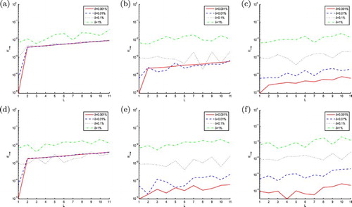
In Figures 1 and 2, the results present the values of $E_{2w}$ and $E_{\mathrm{\infty }w}$ obtained by 3PNDS, 5PNDS and 7PNDS with respect to different time levels $t_j$, respectively, the measured data are added to four various noise levels, where $\delta =0.001\mathrm{\%},\delta =0.01\mathrm{\%},\delta =0.1\mathrm{\%}$ and $\delta =1\mathrm{\%}$ in Example 4.1. When the noise level δ is smaller, it is shown that the numerical results of approximation solutions ${\tilde{w}}^{\delta }(x,t)$ get more accurate among the techniques 3PNDS, 5PNDS and 7PNDS for the following two cases: (a) the spatial-step h becomes smaller; (b) the points number k of the k-step discretization schemes (such as 3PNDS $(k=2)$, 5PNDS $(k=4)$ and 7PNDS $(k=6)$) becomes bigger, but this effect is not obvious as the error level δ is growing. According to Figure 4 and Table 4, it is observed that the approximation source ${\tilde{p}}_{{\alpha }_i}^{\delta }\left(t\right)$ becomes more accurate, as the points number k increases. In addition, the numerical results basically keep unchanged to different noise level δ for taking the same numerical approach and spatial-step h, moreover, when δ becomes smaller, the accuracy of numerical results is generally increasing.

Figure 1. The RMS error of function $w(x,t)$ obtained by 3PNDS, 5PNDS and 7PNDS, respectively, with four different noise levels added to the measured data, namely $\delta =0.001\mathrm{\%},\delta =0.01\mathrm{\%},\delta =0.1\mathrm{\%}$ and $\delta =1\mathrm{\%}$ in Example 4.1. (a) 3PNDS ($h=1/10$), (b) 5PNDS ($h=1/10$), (c) 7PNDS ($h=1/10$), (d) 3PNDS ($h=1/15$), (e) 5PNDS ($h=1/15$) and (f) 7PNDS ($h=1/15$).

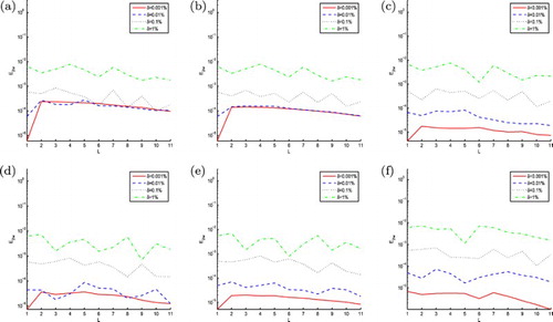
Figure 2. The maximum error of function $w(x,t)$ obtained by 3PNDS, 5PNDS and 7PNDS, respectively, with four different noise levels added to the measured data, namely $\delta =0.001\mathrm{\%},\delta =0.01\mathrm{\%},\delta =0.1\mathrm{\%}$ and $\delta =1\mathrm{\%}$ in Example 4.1. (a) 3PNDS ($h=1/10$), (b) 5PNDS ($h=1/10$), (c) 7PNDS ($h=1/10$), (d) 3PNDS ($h=1/15$), (e) 5PNDS ($h=1/15$) and (f) 7PNDS ($h=1/15$).

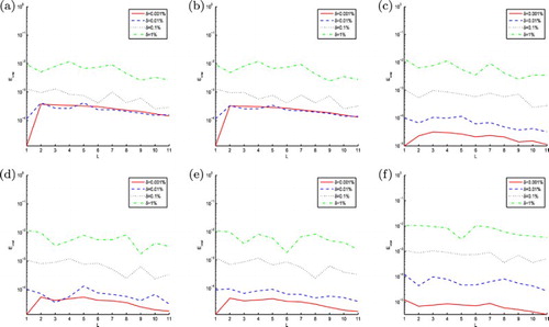
Figure 3. The ratio plots of $w_1$, $w_2$ and $w_3$ for 3PNDS, 5PNDS and 7PNDS, respectively, in Example 4.1, and the numbers ‘$1,2,\dots$’ indicates the expressed sequence for different $h_1$ above. (a) 3PNDS, (b) 5PNDS and (c) 7PNDS.

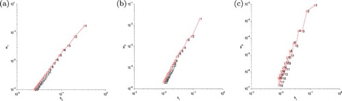
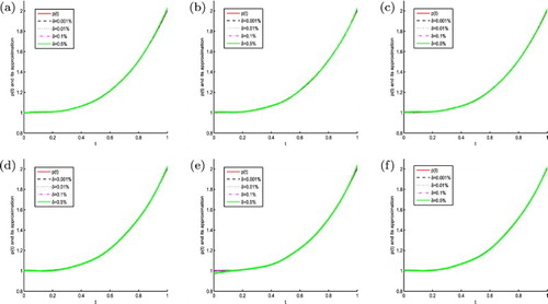
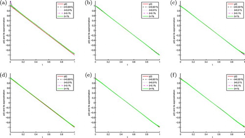
Figure 4. The exact function $p\left(t\right)$ and its approximation for three difference schemes as 3PNDS, 5PNDS and 7PNDS with four different noise levels added to the measured data, namely $\delta =0.001\mathrm{\%},\delta =0.01\mathrm{\%},\delta =0.1\mathrm{\%}$ and $\delta =1\mathrm{\%}$ in Example 4.1. (a) 3PNDS ($h=1/10$), (b) 5PNDS ($h=1/10$), (c) 7PNDS ($h=1/10$), (d) 3PNDS ($h=1/15$), (e) 5PNDS ($h=1/15$) and (f) 7PNDS ($h=1/15$).

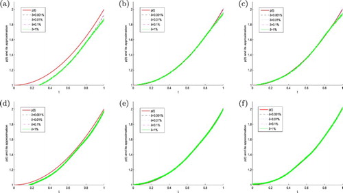
Table 4. The results of $E_{2p}$ and $E_{\mathrm{\infty }p}$ obtained by 3PNDS, 5PNDS, 7PNDS and RBFs, respectively, taking the case of ${\alpha }_i^{\delta }$ in (144(144) ${\alpha }_i^{\delta }=\left[{\left(\frac{\parallel M_1{\parallel }_2}{\parallel M_2{\parallel }_2}\right)}^{{\tilde{n}}_i}\right]{\delta }^{1/2},1\le {\tilde{n}}_i\le {\tilde{N}}_i,$(144) ) for Example 4.1.

		$\delta =0.001\mathrm{\%}$	$\delta =0.01\mathrm{\%}$	$\delta =0.1\mathrm{\%}$	$\delta =1\mathrm{\%}$
3PNDS	$E_{2p}$ ($h=1/10$)	$7.71\times {10}^{-2}$	$7.71\times {10}^{-2}$	$7.73\times {10}^{-2}$	$8.47\times {10}^{-2}$
	$E_{\mathrm{\infty }p}$ ($h=1/10$)	$7.82\times {10}^{-2}$	$7.91\times {10}^{-2}$	$8.21\times {10}^{-2}$	$1.45\times {10}^{-1}$
	$E_{2p}$ ($h=1/15$)	$3.52\times {10}^{-2}$	$3.52\times {10}^{-2}$	$3.53\times {10}^{-2}$	$3.71\times {10}^{-2}$
	$E_{\mathrm{\infty }p}$ ($h=1/15$)	$3.93\times {10}^{-2}$	$4.13\times {10}^{-2}$	$4.78\times {10}^{-2}$	$6.55\times {10}^{-2}$
5PNDS	$E_{2p}$ ($h=1/10$)	$2.69\times {10}^{-3}$	$2.76\times {10}^{-3}$	$3.46\times {10}^{-3}$	$1.42\times {10}^{-2}$
	$E_{\mathrm{\infty }p}$ ($h=1/10$)	$5.67\times {10}^{-3}$	$7.17\times {10}^{-3}$	$1.68\times {10}^{-2}$	$6.68\times {10}^{-2}$
	$E_{2p}$ ($h=1/15$)	$1.05\times {10}^{-3}$	$1.31\times {10}^{-3}$	$2.81\times {10}^{-3}$	$1.06\times {10}^{-2}$
	$E_{\mathrm{\infty }p}$ ($h=1/15$)	$5.03\times {10}^{-3}$	$6.43\times {10}^{-3}$	$1.57\times {10}^{-2}$	$3.03\times {10}^{-2}$
7PNDS	$E_{2p}$ ($h=1/10$)	$1.51\times {10}^{-3}$	$1.64\times {10}^{-3}$	$3.07\times {10}^{-3}$	$1.57\times {10}^{-2}$
	$E_{\mathrm{\infty }p}$ ($h=1/10$)	$4.08\times {10}^{-3}$	$5.80\times {10}^{-3}$	$1.75\times {10}^{-2}$	$7.42\times {10}^{-2}$
	$E_{2p}$ ($h=1/15$)	$9.50\times {10}^{-4}$	$1.24\times {10}^{-3}$	$2.08\times {10}^{-3}$	$9.57\times {10}^{-3}$
	$E_{\mathrm{\infty }p}$ ($h=1/15$)	$4.84\times {10}^{-3}$	$6.39\times {10}^{-3}$	$1.24\times {10}^{-2}$	$3.34\times {10}^{-2}$
RBFs	$E_{2p}$ ($h=1/10$)	$5.92\times {10}^{-3}$	$5.93\times {10}^{-3}$	$5.79\times {10}^{-3}$	$1.06\times {10}^{-2}$
	$E_{\mathrm{\infty }p}$ ($h=1/10$)	$2.60\times {10}^{-2}$	$2.61\times {10}^{-2}$	$2.72\times {10}^{-2}$	$4.13\times {10}^{-2}$

Example 4.2

We consider the second problem (1(1) $\frac{\mathrm{\partial }w}{\mathrm{\partial }t}=\frac{{\mathrm{\partial }}^{2}w}{\mathrm{\partial }{x}^2}+p\left(t\right)w+\varphi (x,t),0<x<1,0<t\le T,$(1) )–(5(5) $w(x^{\ast },t)=E\left(t\right),0\le t\le T,$(5) ): $\begin{array}{rl}\varphi (x,t)& =-\exp (-t)(2+t^3+(1+t^3)\cos (x\left)\right),\\ f\left(x\right)& =\cos \left(x\right)+1,\\ g_0\left(t\right)& =2\exp (-t),\\ g_1\left(t\right)& =\exp (-t)(\cos 1+1),\\ x^{\ast }& =\pi /4,\\ E\left(t\right)& =\exp (-t)(\sqrt{2}/2+1),\end{array}$ and Example 4.2 has the exact solution $\begin{array}{rl}w(x,t)& =\exp (-t)(\cos (x)+1),\\ p\left(t\right)& =1+t^3.\end{array}$

In Figures 5 and 6, the numerical results display the values of $E_{2w}$ and $E_{\mathrm{\infty }w}$ derived by 3PNDS, 5PNDS and 7PNDS with respect to different time levels $t_j$, respectively, the measured data are added to four different error levels, namely $\delta =0.001\mathrm{\%},\delta =0.01\mathrm{\%},\delta =0.1\mathrm{\%}$ and $\delta =0.5\mathrm{\%}$ in Example 4.2. It is shown that the accuracy of approximation ${\tilde{w}}^{\delta }(x,t)$ becomes higher, when the noise level δ is smaller. We show that the accuracy of approximation ${\tilde{p}}_{{\alpha }_i}^{\delta }\left(t\right)$ is getting more accurate and more stable, when the noise level δ becomes smaller by Figure 8 and Table 6. Furthermore, the illustrated results of ${\tilde{p}}_{{\alpha }_i}^{\delta }\left(t\right)$ are also satisfactory and effective with the reduction of spatial-step h.

Figure 5. The RMS error of function $w(x,t)$ obtained by 3PNDS, 5PNDS and 7PNDS, respectively, with four different noise levels added to the measured data, namely $\delta =0.001\mathrm{\%},\delta =0.01\mathrm{\%},\delta =0.1\mathrm{\%}$ and $\delta =0.5\mathrm{\%}$ in Example 4.2. (a) 3PNDS ($h=1/10$), (b) 5PNDS ($h=1/10$), (c) 7PNDS ($h=1/10$), (d) 3PNDS ($h=1/15$), (e) 5PNDS ($h=1/15$) and (f) 7PNDS ($h=1/15$).

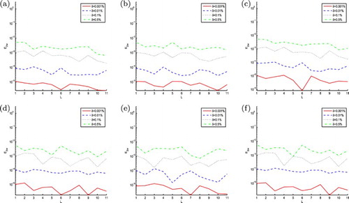
Figure 6. The maximum error of function $w(x,t)$ obtained by 3PNDS, 5PNDS and 7PNDS, respectively, with four different noise levels added to the measured data, namely $\delta =0.001\mathrm{\%},\delta =0.01\mathrm{\%},\delta =0.1\mathrm{\%}$ and $\delta =0.5\mathrm{\%}$ in Example 4.2. (a) 3PNDS ($h=1/10$), (b) 5PNDS ($h=1/10$), (c) 7PNDS ($h=1/10$), (d) 3PNDS ($h=1/15$), (e) 5PNDS ($h=1/15$) and (f) 7PNDS ($h=1/15$).

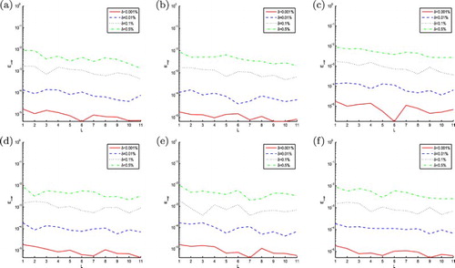
Figure 7. The ratio plots of $w_1$, $w_2$ and $w_3$ for 3PNDS, 5PNDS and 7PNDS, respectively, in Example 4.2, and the numbers ‘$1,2,\dots$’ indicate the expressed sequence for different $h_1$ above. (a) 3PNDS, (b) 5PNDS and (c) 7PNDS.

Figure 8. The exact function $p\left(t\right)$ and its approximation for three difference schemes as 3PNDS, 5PNDS and 7PNDS with four different noise levels added to the measured data, namely $\delta =0.001\mathrm{\%},\delta =0.01\mathrm{\%},\delta =0.1\mathrm{\%}$ and $\delta =0.5\mathrm{\%}$ in Example 4.2. (a) 3PNDS ($h=1/10$), (b) 5PNDS ($h=1/10$), (c) 7PNDS ($h=1/10$), (d) 3PNDS ($h=1/15$), (e) 5PNDS ($h=1/15$) and (f) 7PNDS ($h=1/15$).

Example 4.3

We consider the third problem (1(1) $\frac{\mathrm{\partial }w}{\mathrm{\partial }t}=\frac{{\mathrm{\partial }}^{2}w}{\mathrm{\partial }{x}^2}+p\left(t\right)w+\varphi (x,t),0<x<1,0<t\le T,$(1) )–(5(5) $w(x^{\ast },t)=E\left(t\right),0\le t\le T,$(5) ): $\begin{array}{rl}\varphi (x,t)& =({\pi }^2+2t)\exp \left(t\right)\cos \left(\pi x\right)+2xt\exp \left(t\right),\\ f\left(x\right)& =x+\cos \left(\pi x\right),\\ g_0\left(t\right)& =\exp \left(t\right),\\ g_1\left(t\right)& =0,\\ x^{\ast }& =2/3,\\ E\left(t\right)& =\exp \left(t\right)/6,\end{array}$ and Example 4.3 has the exact solution $\begin{array}{rl}w(x,t)& =\exp \left(t\right)(\cos (\pi x)+x),\\ p\left(t\right)& =1-2t.\end{array}$

The numerical results display the values of $E_{2w}$ and $E_{\mathrm{\infty }w}$ derived by 3PNDS, 5PNDS and 7PNDS with respect to different time levels $t_j$ by Figures 9 and 10, respectively; the measured data are added to four different error levels, namely $\delta =0.001\mathrm{\%},\delta =0.01\mathrm{\%},\delta =0.1\mathrm{\%}$ and $\delta =1\mathrm{\%}$ in Example 4.3. It is observed that the results of approximation solution ${\tilde{w}}^{\delta }(x,t)$ become more accurate, when the spatial-step h is smaller and the points number k ( k-step nodes) increases. Besides, the accuracy of ${\tilde{w}}^{\delta }(x,t)$ depends on the noise level δ according to the above three tests, if the selection of δ is a smaller value, the numerical solutions work effectively in this paper. In Figure 12 and Table 8, the numerical results of approximation ${\tilde{p}}_{{\alpha }_i}^{\delta }\left(t\right)$ are stable by the choice of some appropriate factors, such as the noise level δ, the regularization parameters ${\alpha }_i^{\delta }$, the spatial-step h and the points number k.

Figure 9. The RMS error of function $w(x,t)$ obtained by 3PNDS, 5PNDS and 7PNDS, respectively, with four different noise levels added to the measured data, namely $\delta =0.001\mathrm{\%},\delta =0.01\mathrm{\%},\delta =0.1\mathrm{\%}$ and $\delta =1\mathrm{\%}$ in Example 4.3. (a) 3PNDS ($h=1/10$), (b) 5PNDS ($h=1/10$), (c) 7PNDS ($h=1/10$), (d) 3PNDS ($h=1/15$), (e) 5PNDS ($h=1/15$) and (f) 7PNDS ($h=1/15$).

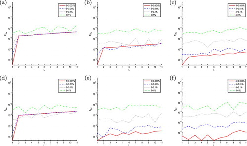
Figure 10. The maximum error of function $w(x,t)$ obtained by 3PNDS, 5PNDS and 7PNDS, respectively, with four different noise levels added to the measured data, namely $\delta =0.001\mathrm{\%},\delta =0.01\mathrm{\%},\delta =0.1\mathrm{\%}$ and $\delta =1\mathrm{\%}$ in Example 4.3. (a) 3PNDS ($h=1/10$), (b) 5PNDS ($h=1/10$), (c) 7PNDS ($h=1/10$), (d) 3PNDS ($h=1/15$), (e) 5PNDS ($h=1/15$) and (f) 7PNDS ($h=1/15$).

In the theoretical analysis, when the regularization parameters ${\alpha }_i^{\delta }={\delta }^{1/2}$, we can obtain the corresponding orders of convergence. As mentioned before, the rule is not a suitable choice for practical applications. We also give the numerical results in Tables 5, 7 and 9, which are obtained by the choice rule ${\alpha }_i^{\delta }={\delta }^{1/2}$. In comparison, it is clear that the results obtained by the heuristic choice (144(144) ${\alpha }_i^{\delta }=\left[{\left(\frac{\parallel M_1{\parallel }_2}{\parallel M_2{\parallel }_2}\right)}^{{\tilde{n}}_i}\right]{\delta }^{1/2},1\le {\tilde{n}}_i\le {\tilde{N}}_i,$(144) ) are better, as shown in Tables 4, 6 and 8.

Table 5. The results of $E_{2p}$ and $E_{\mathrm{\infty }p}$ obtained by 3PNDS, 5PNDS and 7PNDS, respectively, taking the case of ${\alpha }_i^{\delta }={\delta }^{1/2}$ for Example 4.1.

		$\delta =0.001\mathrm{\%}$	$\delta =0.01\mathrm{\%}$	$\delta =0.1\mathrm{\%}$	$\delta =1\mathrm{\%}$
3PNDS	$E_{2p}$ ($h=1/10$)	$8.16\times {10}^{-2}$	$8.16\times {10}^{-2}$	$8.21\times {10}^{-2}$	$8.63\times {10}^{-2}$
	$E_{\mathrm{\infty }p}$ ($h=1/10$)	$1.43\times {10}^{-1}$	$1.43\times {10}^{-1}$	$1.43\times {10}^{-1}$	$1.46\times {10}^{-1}$
	$E_{2p}$ ($h=1/15$)	$4.33\times {10}^{-2}$	$4.33\times {10}^{-2}$	$4.32\times {10}^{-2}$	$4.26\times {10}^{-2}$
	$E_{\mathrm{\infty }p}$ ($h=1/15$)	$1.05\times {10}^{-1}$	$1.05\times {10}^{-1}$	$1.05\times {10}^{-1}$	$1.07\times {10}^{-1}$
5PNDS	$E_{2p}$ ($h=1/10$)	$2.03\times {10}^{-2}$	$2.03\times {10}^{-2}$	$2.04\times {10}^{-2}$	$2.20\times {10}^{-2}$
	$E_{\mathrm{\infty }p}$ ($h=1/10$)	$7.20\times {10}^{-2}$	$7.21\times {10}^{-2}$	$7.23\times {10}^{-2}$	$7.49\times {10}^{-2}$
	$E_{2p}$ ($h=1/15$)	$2.03\times {10}^{-2}$	$2.03\times {10}^{-2}$	$2.04\times {10}^{-2}$	$2.14\times {10}^{-2}$
	$E_{\mathrm{\infty }p}$ ($h=1/15$)	$7.29\times {10}^{-2}$	$7.30\times {10}^{-2}$	$7.35\times {10}^{-2}$	$7.22\times {10}^{-2}$
7PNDS	$E_{2p}$ ($h=1/10$)	$2.05\times {10}^{-2}$	$2.05\times {10}^{-2}$	$2.05\times {10}^{-2}$	$2.23\times {10}^{-2}$
	$E_{\mathrm{\infty }p}$ ($h=1/10$)	$7.32\times {10}^{-2}$	$7.32\times {10}^{-2}$	$7.32\times {10}^{-2}$	$7.80\times {10}^{-2}$
	$E_{2p}$ ($h=1/15$)	$2.03\times {10}^{-2}$	$2.04\times {10}^{-2}$	$2.04\times {10}^{-2}$	$2.13\times {10}^{-2}$
	$E_{\mathrm{\infty }p}$ ($h=1/15$)	$7.31\times {10}^{-2}$	$7.32\times {10}^{-2}$	$7.39\times {10}^{-2}$	$7.60\times {10}^{-2}$

Table 6. The results of $E_{2p}$ and $E_{\mathrm{\infty }p}$ obtained by 3PNDS, 5PNDS, 7PNDS and RBFs, respectively, taking the case of ${\alpha }_i^{\delta }$ in (144(144) ${\alpha }_i^{\delta }=\left[{\left(\frac{\parallel M_1{\parallel }_2}{\parallel M_2{\parallel }_2}\right)}^{{\tilde{n}}_i}\right]{\delta }^{1/2},1\le {\tilde{n}}_i\le {\tilde{N}}_i,$(144) ) for Example 4.2.

		$\delta =0.001\mathrm{\%}$	$\delta =0.01\mathrm{\%}$	$\delta =0.1\mathrm{\%}$	$\delta =0.5\mathrm{\%}$
3PNDS	$E_{2p}$ ($h=1/10$)	$9.41\times {10}^{-4}$	$1.10\times {10}^{-3}$	$1.48\times {10}^{-3}$	$6.40\times {10}^{-3}$
	$E_{\mathrm{\infty }p}$ ($h=1/10$)	$1.92\times {10}^{-3}$	$2.91\times {10}^{-3}$	$7.64\times {10}^{-3}$	$3.10\times {10}^{-2}$
	$E_{2p}$ ($h=1/15$)	$7.42\times {10}^{-4}$	$1.03\times {10}^{-3}$	$1.74\times {10}^{-3}$	$5.63\times {10}^{-3}$
	$E_{\mathrm{\infty }p}$ ($h=1/15$)	$5.76\times {10}^{-3}$	$7.85\times {10}^{-3}$	$1.16\times {10}^{-2}$	$2.77\times {10}^{-2}$
5PNDS	$E_{2p}$ ($h=1/10$)	$1.32\times {10}^{-3}$	$1.45\times {10}^{-3}$	$1.80\times {10}^{-3}$	$5.81\times {10}^{-3}$
	$E_{\mathrm{\infty }p}$ ($h=1/10$)	$2.74\times {10}^{-3}$	$5.08\times {10}^{-3}$	$1.09\times {10}^{-2}$	$2.66\times {10}^{-2}$
	$E_{2p}$ ($h=1/15$)	$8.60\times {10}^{-4}$	$1.13\times {10}^{-3}$	$2.19\times {10}^{-3}$	$8.08\times {10}^{-3}$
	$E_{\mathrm{\infty }p}$ ($h=1/15$)	$5.97\times {10}^{-3}$	$8.28\times {10}^{-3}$	$1.14\times {10}^{-2}$	$3.78\times {10}^{-2}$
7PNDS	$E_{2p}$ ($h=1/10$)	$1.31\times {10}^{-3}$	$1.43\times {10}^{-3}$	$1.68\times {10}^{-3}$	$5.95\times {10}^{-3}$
	$E_{\mathrm{\infty }p}$ ($h=1/10$)	$2.29\times {10}^{-3}$	$3.73\times {10}^{-3}$	$6.78\times {10}^{-3}$	$2.31\times {10}^{-2}$
	$E_{2p}$ ($h=1/15$)	$8.54\times {10}^{-4}$	$1.12\times {10}^{-3}$	$1.84\times {10}^{-3}$	$5.31\times {10}^{-3}$
	$E_{\mathrm{\infty }p}$ ($h=1/15$)	$5.94\times {10}^{-3}$	$8.02\times {10}^{-3}$	$1.21\times {10}^{-2}$	$2.10\times {10}^{-2}$
RBFs	$E_{2p}$ ($h=1/10$)	$4.62\times {10}^{-3}$	$4.63\times {10}^{-3}$	$4.56\times {10}^{-3}$	$8.40\times {10}^{-3}$
	$E_{\mathrm{\infty }p}$ ($h=1/10$)	$2.50\times {10}^{-2}$	$2.49\times {10}^{-2}$	$2.59\times {10}^{-2}$	$3.45\times {10}^{-2}$

Table 7. The results of $E_{2p}$ and $E_{\mathrm{\infty }p}$ obtained by 3PNDS, 5PNDS and 7PNDS, respectively, taking the case of ${\alpha }_i^{\delta }={\delta }^{1/2}$ for Example 4.2.

		$\delta =0.001\mathrm{\%}$	$\delta =0.01\mathrm{\%}$	$\delta =0.1\mathrm{\%}$	$\delta =0.5\mathrm{\%}$
3PNDS	$E_{2p}$ ($h=1/10$)	$7.15\times {10}^{-2}$	$7.18\times {10}^{-2}$	$7.23\times {10}^{-2}$	$7.30\times {10}^{-2}$
	$E_{\mathrm{\infty }p}$ ($h=1/10$)	$1.92\times {10}^{-1}$	$1.93\times {10}^{-1}$	$1.95\times {10}^{-1}$	$2.02\times {10}^{-1}$
	$E_{2p}$ ($h=1/15$)	$7.17\times {10}^{-2}$	$7.19\times {10}^{-2}$	$7.20\times {10}^{-2}$	$7.03\times {10}^{-2}$
	$E_{\mathrm{\infty }p}$ ($h=1/15$)	$1.92\times {10}^{-1}$	$1.93\times {10}^{-1}$	$1.96\times {10}^{-1}$	$1.91\times {10}^{-1}$
5PNDS	$E_{2p}$ ($h=1/10$)	$7.14\times {10}^{-2}$	$7.17\times {10}^{-2}$	$7.19\times {10}^{-2}$	$7.14\times {10}^{-2}$
	$E_{\mathrm{\infty }p}$ ($h=1/10$)	$1.92\times {10}^{-1}$	$1.93\times {10}^{-1}$	$1.95\times {10}^{-1}$	$2.00\times {10}^{-1}$
	$E_{2p}$ ($h=1/15$)	$7.16\times {10}^{-2}$	$7.19\times {10}^{-2}$	$7.24\times {10}^{-2}$	$7.16\times {10}^{-2}$
	$E_{\mathrm{\infty }p}$ ($h=1/15$)	$1.92\times {10}^{-1}$	$1.93\times {10}^{-1}$	$1.97\times {10}^{-1}$	$2.00\times {10}^{-1}$
7PNDS	$E_{2p}$ ($h=1/10$)	$7.14\times {10}^{-2}$	$7.17\times {10}^{-2}$	$7.17\times {10}^{-2}$	$7.26\times {10}^{-2}$
	$E_{\mathrm{\infty }p}$ ($h=1/10$)	$1.92\times {10}^{-1}$	$1.93\times {10}^{-1}$	$1.93\times {10}^{-1}$	$2.02\times {10}^{-1}$
	$E_{2p}$ ($h=1/15$)	$7.16\times {10}^{-2}$	$7.19\times {10}^{-2}$	$7.21\times {10}^{-2}$	$7.09\times {10}^{-2}$
	$E_{\mathrm{\infty }p}$ ($h=1/15$)	$1.92\times {10}^{-1}$	$1.93\times {10}^{-1}$	$1.96\times {10}^{-1}$	$1.94\times {10}^{-1}$

Table 8. The results of $E_{2p}$ and $E_{\mathrm{\infty }p}$ obtained by 3PNDS, 5PNDS, 7PNDS and RBFs, respectively, taking the case of ${\alpha }_i^{\delta }$ in (144(144) ${\alpha }_i^{\delta }=\left[{\left(\frac{\parallel M_1{\parallel }_2}{\parallel M_2{\parallel }_2}\right)}^{{\tilde{n}}_i}\right]{\delta }^{1/2},1\le {\tilde{n}}_i\le {\tilde{N}}_i,$(144) ) for Example 4.3.

		$\delta =0.001\mathrm{\%}$	$\delta =0.01\mathrm{\%}$	$\delta =0.1\mathrm{\%}$	$\delta =1\mathrm{\%}$
3PNDS	$E_{2p}$ ($h=1/10$)	$4.00\times {10}^{-2}$	$4.04\times {10}^{-2}$	$3.99\times {10}^{-2}$	$3.34\times {10}^{-2}$
	$E_{\mathrm{\infty }p}$ ($h=1/10$)	$2.23\times {10}^{-1}$	$2.12\times {10}^{-1}$	$2.16\times {10}^{-1}$	$6.16\times {10}^{-2}$
	$E_{2p}$ ($h=1/15$)	$1.61\times {10}^{-2}$	$1.60\times {10}^{-2}$	$1.61\times {10}^{-2}$	$1.56\times {10}^{-2}$
	$E_{\mathrm{\infty }p}$ ($h=1/15$)	$2.56\times {10}^{-2}$	$2.94\times {10}^{-2}$	$3.33\times {10}^{-2}$	$3.87\times {10}^{-2}$
5PNDS	$E_{2p}$ ($h=1/10$)	$3.33\times {10}^{-3}$	$3.42\times {10}^{-3}$	$4.56\times {10}^{-3}$	$7.00\times {10}^{-3}$
	$E_{\mathrm{\infty }p}$ ($h=1/10$)	$5.39\times {10}^{-3}$	$7.77\times {10}^{-3}$	$2.34\times {10}^{-2}$	$2.43\times {10}^{-2}$
	$E_{2p}$ ($h=1/15$)	$1.53\times {10}^{-3}$	$2.26\times {10}^{-3}$	$3.15\times {10}^{-3}$	$6.37\times {10}^{-3}$
	$E_{\mathrm{\infty }p}$ ($h=1/15$)	$9.99\times {10}^{-3}$	$1.39\times {10}^{-2}$	$2.00\times {10}^{-2}$	$3.82\times {10}^{-2}$
7PNDS	$E_{2p}$ ($h=1/10$)	$1.58\times {10}^{-3}$	$1.62\times {10}^{-3}$	$3.83\times {10}^{-3}$	$1.03\times {10}^{-2}$
	$E_{\mathrm{\infty }p}$ ($h=1/10$)	$2.96\times {10}^{-3}$	$2.97\times {10}^{-3}$	$2.20\times {10}^{-2}$	$6.32\times {10}^{-2}$
	$E_{2p}$ ($h=1/15$)	$1.48\times {10}^{-3}$	$2.22\times {10}^{-3}$	$3.57\times {10}^{-3}$	$7.48\times {10}^{-3}$
	$E_{\mathrm{\infty }p}$ ($h=1/15$)	$9.81\times {10}^{-3}$	$1.35\times {10}^{-2}$	$2.23\times {10}^{-2}$	$3.65\times {10}^{-2}$
RBFs	$E_{2p}$ ($h=1/10$)	$1.26\times {10}^{-3}$	$1.28\times {10}^{-3}$	$2.04\times {10}^{-3}$	$1.07\times {10}^{-2}$
	$E_{\mathrm{\infty }p}$ ($h=1/10$)	$6.19\times {10}^{-3}$	$6.36\times {10}^{-3}$	$1.24\times {10}^{-2}$	$3.86\times {10}^{-2}$

Table 9. The results of $E_{2p}$ and $E_{\mathrm{\infty }p}$ obtained by 3PNDS, 5PNDS and 7PNDS, respectively, taking the case of ${\alpha }_i^{\delta }={\delta }^{1/2}$ for Example 4.3.

		$\delta =0.001\mathrm{\%}$	$\delta =0.01\mathrm{\%}$	$\delta =0.1\mathrm{\%}$	$\delta =1\mathrm{\%}$
3PNDS	$E_{2p}$ ($h=1/10$)	$5.30\times {10}^{-2}$	$5.30\times {10}^{-2}$	$5.28\times {10}^{-2}$	$5.20\times {10}^{-2}$
	$E_{\mathrm{\infty }p}$ ($h=1/10$)	$1.48\times {10}^{-1}$	$1.48\times {10}^{-1}$	$1.48\times {10}^{-1}$	$1.49\times {10}^{-1}$
	$E_{2p}$ ($h=1/15$)	$4.55\times {10}^{-2}$	$4.55\times {10}^{-2}$	$4.55\times {10}^{-2}$	$4.59\times {10}^{-2}$
	$E_{\mathrm{\infty }p}$ ($h=1/15$)	$1.40\times {10}^{-1}$	$1.40\times {10}^{-1}$	$1.40\times {10}^{-1}$	$1.48\times {10}^{-1}$
5PNDS	$E_{2p}$ ($h=1/10$)	$4.32\times {10}^{-2}$	$4.32\times {10}^{-2}$	$4.32\times {10}^{-2}$	$4.20\times {10}^{-2}$
	$E_{\mathrm{\infty }p}$ ($h=1/10$)	$1.34\times {10}^{-1}$	$1.34\times {10}^{-1}$	$1.34\times {10}^{-1}$	$1.34\times {10}^{-1}$
	$E_{2p}$ ($h=1/15$)	$4.30\times {10}^{-2}$	$4.30\times {10}^{-2}$	$4.29\times {10}^{-2}$	$4.34\times {10}^{-2}$
	$E_{\mathrm{\infty }p}$ ($h=1/15$)	$1.32\times {10}^{-1}$	$1.32\times {10}^{-1}$	$1.32\times {10}^{-1}$	$1.44\times {10}^{-1}$
7PNDS	$E_{2p}$ ($h=1/10$)	$4.31\times {10}^{-2}$	$4.31\times {10}^{-2}$	$4.32\times {10}^{-2}$	$4.24\times {10}^{-2}$
	$E_{\mathrm{\infty }p}$ ($h=1/10$)	$1.33\times {10}^{-1}$	$1.33\times {10}^{-1}$	$1.33\times {10}^{-1}$	$1.38\times {10}^{-1}$
	$E_{2p}$ ($h=1/15$)	$4.30\times {10}^{-2}$	$4.30\times {10}^{-2}$	$4.29\times {10}^{-2}$	$4.32\times {10}^{-2}$
	$E_{\mathrm{\infty }p}$ ($h=1/15$)	$1.32\times {10}^{-1}$	$1.32\times {10}^{-1}$	$1.32\times {10}^{-1}$	$1.39\times {10}^{-1}$

In addition, according to Figures 3, 7 and 11, we know that the inclination of the images, which are obtained by computing the ratios $w_1$, $w_2$ and $w_3$ at the point $(h_1,{\tau }_1)$, gets bigger through three numerical approaches as 3PNDS, 5PNDS and 7PNDS, it means that the convergence rate of the presented methods should be generally improved with increasing of the points number k ( k-step nodes).

Figure 11. The ratio plots of $w_1$, $w_2$ and $w_3$ for 3PNDS, 5PNDS and 7PNDS, respectively, in Example 4.3, and the numbers ‘$1,2,\dots$’ indicate the expressed sequence for different $h_1$ above. (a) 3PNDS, (b) 5PNDS and (c) 7PNDS.

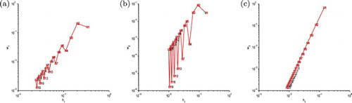
Figure 12. The exact function $p\left(t\right)$ and its approximation for three difference schemes as 3PNDS, 5PNDS and 7PNDS with four different noise levels added to the measured data, namely $\delta =0.001\mathrm{\%},\delta =0.01\mathrm{\%},\delta =0.1\mathrm{\%}$ and $\delta =1\mathrm{\%}$ in Example 4.3. (a) 3PNDS ($h=1/10$), (b) 5PNDS ($h=1/10$), (c) 7PNDS ($h=1/10$), (d) 3PNDS ($h=1/15$), (e) 5PNDS ($h=1/15$) and (f) 7PNDS ($h=1/15$).

5. Conclusion

In this paper, we construct a family of multistep numerical difference schemes, which are applied in the one-dimensional parabolic inverse problem with a control parameter $p\left(t\right)$. Specially, we construct three difference schemes 3PNDS, 5PNDS and 7PNDS, and develop their corresponding truncation error estimations and convergence conclusions. It is well known that the problem of numerical differentiation with noisy errors is mildly ill-posed, we use the smoothing spline based on the Tikhonov regularization technique to obtain stable approximation solutions. The numerical results are given to observe that the accuracy of ${\tilde{w}}^{\delta }(x,t)$ and ${\tilde{p}}_{{\alpha }_i}^{\delta }\left(t\right)$ depends on the selection of some factors, such as the noise level δ, the regularization parameters ${\alpha }_i^{\delta }$, the time-step τ, the spatial-step h and the points number k (k-step nodes). If the step sizes τ, h, and the noise level δ are decreased, thus the approximation solutions ${\tilde{w}}^{\delta }(x,t)$ and ${\tilde{p}}_{{\alpha }_i}^{\delta }\left(t\right)$ can get more accurate results. If the step sizes h, τ, and the noise level δ are chosen much more smaller, thus the approximation solution ${\tilde{p}}_{{\alpha }_i}^{\delta }\left(t\right)$ can get more accurate results, however, it would require more computational cost in this case, we will improve this in our further work. In conclusion, the presented numerical schemes are stable and effective.

Disclosure statement

No potential conflict of interest was reported by the authors.

Additional information

Funding

This work was supported by the National Natural Science Foundation of China (Nos. 11471066, 11290143, 11572081), the Fundamental Research of Civil Aircraft (No. MJ-F-2012-04), the Fundamental Research Funds for the Central Universities (DUT15LK44), the Scientific Research Funds of Inner Mongolia University for the Nationalities (NMDYB17154) and PhD research startup foundation of Inner Mongolia University for Nationalities (BS424).

References

- Hon YC, Wei T. A fundamental solution method for inverse heat conduction problem. Eng Anal Bound Elem. 2004;28:489–495. doi: 10.1016/S0955-7997(03)00102-4
- Hansen PC. Regularization tools: a Matlab package for analysis and solution of discrete ill-posed problems. Numer Algorithms. 1994;6:1–35. doi: 10.1007/BF02149761
- Cheng J, Yamamoto M. One new strategy for a priori choice of regularizing parameters in Tikhonov's regularization. Inverse Probl. 2000;16:31–38. doi: 10.1088/0266-5611/16/4/101
- Tikhonov AN, Arsenin VY. Solutions of ill-posed problems. Washington (DC), New York: V.H. Winston & Sons, John Wiley & Sons; 1977.
- Dehghan M. Numerical solution of one-dimensional parabolic inverse problem. Appl Math Comput. 2003;136:333–344.
- Dehghan M. Finding a control parameter in one-dimensional parabolic equations. Appl Math Comput. 2003;135:491–503.
- Dehghan M. An inverse problem of finding a source parameter in a semilinear parabolic equation. Appl Math Model. 2001;25:743–754. doi: 10.1016/S0307-904X(01)00010-5
- Cannon JR, Lin YP, Xu SZ. Numerical procedures for the determination of an unknown coefficient in semi-linear parabolic differential equations. Inverse Probl. 1994;10:227–243. doi: 10.1088/0266-5611/10/2/004
- Dehghan M. Parameter determination in a partial differential equation from the overspecified data. Math Comput Model. 2005;41:196–213. doi: 10.1016/j.mcm.2004.07.010
- Mitchell AR, Griffiths DF. The finite difference method in partial differential equations. New York: Wiley; 1980.
- Tatari M, Dehghan M. A method for solving partial differential equations via radial basis functions: application to the heat equation. Eng Anal Bound Elem. 2010;34:206–212. doi: 10.1016/j.enganabound.2009.09.003
- Chen W, Tanaka M. A meshless, integration-free, and boundary-only RBF technique. Comput Math Appl. 2002;43:379–391. doi: 10.1016/S0898-1221(01)00293-0
- Dehghan M, Tatari M. Determination of a control parameter in a one-dimensional parabolic equation using the method of radial basis function. Math Comput Model. 2006;44:1160–1168. doi: 10.1016/j.mcm.2006.04.003
- Ma LM, Wu ZM. Radial basis functions method for parabolic inverse problem. Int J Comput Math. 2011;88(2):384–395. doi: 10.1080/00207160903452236
- Arghand M, Amirfakhrian M. A meshless method based on the fundamental solution and radial basis function for solving an inverse heat conduction. Adv Math Phys. 2015;2015:1–8. Article ID 256726. doi: 10.1155/2015/256726
- Hon YC, Wei T. The method of fundamental solution for solving multidimensional inverse heat conduction problems. Comput Model Eng Sci. 2005;7(2):119–132.
- Dong CF, Sun FY, Meng BQ. A method of fundamental solutions for inverse heat conduction problems in an anisotropic medium. Eng Anal Bound Elem. 2007;31:75–82. doi: 10.1016/j.enganabound.2006.04.007
- Shen SY. A numerical study of inverse heat conduction problems. Comput Math Appl. 1999;38:173–188. doi: 10.1016/S0898-1221(99)00248-5
- Johansson T, Lesnic D. Determination of a spacewise dependent heat source. J Comput Appl Math. 2007;209:66–80. doi: 10.1016/j.cam.2006.10.026
- Dehghan M. Implicit solution of a two-dimensional parabolic inverse problem with temperature overspecification. J Comput Anal Appl. 2001;3(4):383–398.
- Dehghan M. Finite difference schemes for two-dimensional parabolic inverse problem with temperature overspecification. Int J Comput Math. 2000;75:339–349. doi: 10.1080/00207160008804989
- Chantasiriwan S. An algorithm for solving multidimensional inverse heat conduction problem. Int J Heat Mass Transf. 2001;44:3823–3832. doi: 10.1016/S0017-9310(01)00037-0
- Dehghan M. Determination of a control function in three-dimensional parabolic equations. Math Comput Simul. 2003;61:89–100. doi: 10.1016/S0378-4754(01)00434-7
- Dehghan M, Abbaszadeh M, Mohebbi A. The numerical solution of nonlinear high dimensional generalized Benjamin–Bona–Mahony–Burgers equation via the meshless method of radial basis function. Comput Math Appl. 2014;68:212–237. doi: 10.1016/j.camwa.2014.05.019
- Dehghan M, Mohammadi V. The numerical solution of Cahn–Hilliard (CH) equation in one, two and three-dimensions via globally radial basis functions (GRBFs) and RBFs-differential quadrature (RBFs-DQ) methods. Eng Anal Bound Elem. 2015;51:74–100. doi: 10.1016/j.enganabound.2014.10.008
- Lakestani M, Dehghan M. The use of Chebyshev cardinal functions for the solution of a partial differential equation with an unknown time-dependent coefficient subject to an extra measurement. J Comput Appl Math. 2010;235:669–678. doi: 10.1016/j.cam.2010.06.020
- Mohebbi A, Dehghan M. High-order scheme for determination of a control parameter in an inverse problem from the over-specified data. Comput Phys Comm. 2010;181:1947–1954. doi: 10.1016/j.cpc.2010.09.009
- Dehghan M. Fourth-order techniques for identifying a control parameter in the parabolic equations. Int J Eng Sci. 2002;40(4):433–447. doi: 10.1016/S0020-7225(01)00066-0
- Dehghan M, Shakeri F. Method of lines solutions of the parabolic inverse problem with an overspecification at a point. Numer Algorithms. 2009;50(4):417–437. doi: 10.1007/s11075-008-9234-3
- Shamsi M, Dehghan M. Determination of a control function in three-dimensional parabolic equations by Legendre pseudospectral method. Numer Methods Partial Differ Equ. 2012;28(1):74–93. doi: 10.1002/num.20608
- Saadatmandia A, Dehghan M. Computation of two time-dependent coefficients in a parabolic partial differential equation subject to additional specifications. Int J Comput Math. 2010;87(5):997–1008. doi: 10.1080/00207160802253958
- Cannon JR, Duchateau P. An inverse problem for an unknown source in heat equation. J Math Anal Appl. 1980;75:465–485. doi: 10.1016/0022-247X(80)90095-5
- Cannon JR, Lin Y, Wng S. Determination of source parameter in parabolic equation. Meccanica. 1992;27:85–94. doi: 10.1007/BF00420586
- Macbain JA, Bendar JB. Existence and uniqueness properties for the one-dimensional magnetotellurics inversion problem. J Math Phys. 1986;27:645–649. doi: 10.1063/1.527219
- Macbain JA. Inversion theory for a parametrized diffusion problem. SIAM J Appl Math. 1987;47:1386–1391. doi: 10.1137/0147091
- Cannon JR, Lin Y. An inverse problem of finding a parameter in a semi-linear heat equation. J Math Anal Appl. 1990;145:470–484. doi: 10.1016/0022-247X(90)90414-B
- Cannon JR, Lin YP. Determination of a parameter p(t) in some quasi-linear parabolic differential equations. Inverse Probl. 1988;4:35–45. doi: 10.1088/0266-5611/4/1/006
- Cannon JR, Lin YP. Determination of parameter p(t) in Ho¨lder classes for some semilinear parabolic equations. Inverse Probl. 1988;4:595–606. doi: 10.1088/0266-5611/4/3/005
- Li CJ. A kind of multistep finite difference methods for arbitrary order linear boundary value problem. Appl Math Comput. 2008;196:858–865.
- Hanke M, Scherzer O. Inverse problems light: numerical differentiation. Am Math Mon. 2001;108(6):512–521. doi: 10.1080/00029890.2001.11919778
- Wei T, Li M. High order numerical derivatives for one-dimensional scattered noisy data. Appl Math Comput. 2006;175:1744–1759.
- Zhang YF, Li CJ. A Gaussian RBFs method with regularization for the numerical solution of inverse heat conduction problems. Inverse Probl Sci Eng. 2016;24(9):1606–1646. doi: 10.1080/17415977.2015.1131825
- Engl HW, Hanke M, Neubauer A. Regularization of inverse problems. Dordrecht/Boston/London: Kluwer Academic Publishers; 1996.
- Wang YB, Jia XZ, Cheng. J. A numerical differentiation method and its application to reconstruction of discontinuity. Inverse Probl. 2002;18:1461–1476. doi: 10.1088/0266-5611/18/6/301
- Hào DN, Chuong LH, Lesnic. D. Heuristic regularization methods for numerical differentiation. Comput Math Appl. 2012;63:816–826. doi: 10.1016/j.camwa.2011.11.047
- Süli E, Mayers D. An introduction to numerical analysis. Cambridge (UK): Cambridge University Press; 2003.
- Adams RA. Sobolev spaces, pure and applied mathematics. Vol. 65. New York/London: Academic Press; 1975.
- de Boor C. Spline toolbox for use with matlab. Natick: The MathWorks, Inc.; 1992.