Rheometry based on free surface velocity

ABSTRACT

This paper explores the possibility of identifying the rheology of a fluid by monitoring how the free surface velocity field is affected by a perturbation in the flow. The dam-break problem is considered which results from the release of a gate initially separating two fluid pools of different depth. The flow velocity is measured by seeding the free surface with buoyant particles and using Particle Tracking Velocimetry. In parallel, a mathematical model based on the lubrication approximation for fluids with a power-law rheology is developed. The model is validated against a similarity solution which is obtained for the spreading of a gravity current under its own weight and neglecting surface tension. Minimizing the difference between the free surface velocity fields obtained numerically and measured experimentally enables the identification of rheological parameters. The methodology is tested on ideal and noisy synthetic data sets and experimental data obtained with aqueous glycerol.

KEYWORDS:

• Rheology
• dam-break
• free surface data
• parameter identification

MSC SUBJECT CLASSIFICATIONS:

• 76A05
• 76A20

1. Introduction

In a flow bounded by a free surface, perturbations induced by boundary or initial conditions are transferred to the fluid free surface and induce free surface velocity variations. This transfer is dependent on the rheology of the fluid. This study explores the hypothesis that the free surface velocity field is a signature of the fluid rheology and therefore that the fluid rheology can be inferred indirectly by measuring the free surface velocity field. Typically, a rheometer is used to measure the rheology of fluids. However, standard rheometers produce low quality results or do not work at all when the fluid sample is extremely hot (lava), dangerous (nuclear wastes), in too small a quantity (aerosol particles), or inaccessible (remotely observed flows on other planets) [1]. Furthermore, the behaviour of some fluids change when handled, for example snow in an avalanche. It is therefore important to find alternative ways to measure the rheology of fluids in such cases. In this paper, the dam-break problem is considered, which results from the release of a gate initially separating two fluid pools of different depth and the rheological parameters are identified by minimizing the difference between measured and simulated data.

Earlier studies have demonstrated that the rheological behaviour of fluids can be inferred from free surface data by using different techniques. An exhaustive review of these techniques is given in [1] but a brief summary follows. The spreading of a gravity current was considered in Refs [2–4] where it was shown that rheological parameters could be identified by comparing the spreading rate measured experimentally to the one predicted theoretically using a similarity solution analogous to that of Refs [5–7]. The Bostwick and Adams consistometers are also routinely used to estimate the rheology of fluids in the food industry. The idea is to release a fixed amount of fluid down an inclined plane. The rate at which the fluid flows downslope can be related to its rheology, see [8–10]. Recently, Renbaum-Wolff et al. [11–13] developed a new technique to measure the viscosity of small organic aerosol particles, which cannot be measured with standard rheometry techniques. The principle of this technique is to deposit a droplet of material on a substrate and poke it with a sharp needle. The time required for the droplet to relax to its equilibrium shape can be related to its viscosity. The rheology of a fluid can be also be measured by stretching a liquid bridge sandwiched between two parallel plates. As the distance between the plates increases, the liquid bridge thins. The thinning dynamics is well described by a model developed by Eggers [14] and can be related the fluid rheology, see [15,16] for the CaBER system (Capillary Breakup Extensional Rheometer) or [17,18] for the FiSER system (Filament Stretching Extensional Rheometer). Figliuzzi, Jeulin et al. [19] described a method for estimating the rheology of a thin film of paint. This method is based on comparing the observed free surface topography of a thin liquid film at various times with the one computed numerically. Moran and Yeung [20] use the shape recovery of a drop stretched by micropipettes as a proxy to infer its viscosity. Martin and Monnier have shown in [21], that free surface data can be used to infer the rheology of pseudoplastic gravity-driven free-surface flows and the corresponding basal properties for low Reynolds number flows.

In this work, the rheological parameters for Newtonian fluids were identified by measuring the free surface velocity for the dam-break problem with the optimal rheological parameters ascertained to minimize the difference between model and experiment. Section 2 describes the experimental methodology. It is then followed by Section 3 where the mathematical models are presented along with the numerical solution approach. The ability to reconstruct the rheology of ‘synthetic’ and real fluids is assessed in Section 4 and conclusions are drawn in Section 5.

2. Description of the experimental procedure

2.1. Description of the experimental set-up

The experiment was designed to obtain the free surface velocity field for the dam-break problem. The experimental set-up is illustrated in Figure 1. A tank was constructed from Perspex and divided by a removable gate. The gate was a vertical stainless steel sheet that was 255 mm high, 511 mm deep and 1 mm thick. The space between the gate and the tank walls was filled with foam rubber to avoid leakage. The tank was placed inside a dark space on identical double blocks of wood. A black rubber sheet was placed over the bottom of the tank to obtain a black background to facilitate the identification of the white beads. Images were captured with a 1280 × 1024 pixel, 30 frame per second, Motion Studio Motion Pro X3 high speed camera with 55 mm Nikon lens attached. The resolution recorded by the camera was 0.353 mm/pixel. Four fluorescent lights (Phillips 58W/865) were used as a lighting system and placed around two sides of the tank (two tubes on each side). White Acrylic sheets were placed around two sides of the tank in order to diffuse the light and obtain a uniform lighting intensity. The working fluid used in the following is an aqueous glycerol solution (99% glycerol and 1% water). Initially there was a 16 mm difference in fluid depth on either side of the gate with a depth of 26 mm on the upstream side and 10 mm on the downstream side. The tank was placed in a dark area to avoid external light.

Figure 1. Experimental setup- not to scale.

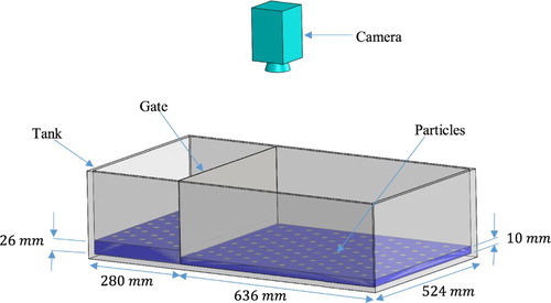
The fluid surface on both sides of the gate was seeded with buoyant, evenly distributed 1 mm diameter polystyrene white beads. The experiment was not started until the fluid on both sides of the gate was observed to be stationary and it was then initiated by the removal of the gate. The height of the camera from the tank base was 1.8 m.

The experimental procedure was as follows:

1. Water was placed inside the tank after each experiment to ensure no leakage from the tank. The gate was placed inside the tank and was sealed tightly to ensure no leakage from its edges. At the conclusion of this stage, the drain system was opened to remove the water from the tank such that the tank was ready for the experiment.

2. A ruler was placed inside the tank to calculate the pixel to millimetres conversion factor.

3. The fluid used in the experiment was then prepared. The depth of the fluid inside the tank was measured using a point gauge. The fluid must be placed in both the upstream and downstream ends of the tank but in different quantities to obtain different fluid levels across the gate.

4. The polystyrene beads were scattered over the surface of the fluid uniformly to avoid coalescence between particles.

5. The camera was set to start recording the motion from the initial state and it was ensured that the particles were stationary before opening the gate.

6. The gate must be pulled to allow the fluid to flow from the high level to the low level.

7. In the current experiments, 1500 frames were captured.

2.2. Particle tracking velocimetry (PTV)

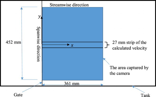
The area inside the tank which was captured by the camera for all the experiments is shown in Figure 2.

Figure 2. Sketch of the area captured by the camera and the central strip over which the velocity profile is averaged.

Particle Tracking Velocimetry (PTV) was used to calculate the free surface velocity from the images captured by the high speed camera. PTV analysis is a process in which individual particles are tracked within a fluid and it was performed using the software package Streams [22].

The velocity data was first computed in the Lagrangian framework using the particle trajectories is shown in Figure 3 and then converted into Eulerian rheological velocities on a rectangular grid.

Figure 3. Particles paths of the aqueous glycerol fluid (displayed in Streams).

In the current experiment 1500 frames were captured for the aqueous glycerol experiment with a 0.03 s time step between frames, ensuring the full motion of the fluid was captured. For each time step, the velocity field was obtained.

2.3. Fluid rheology

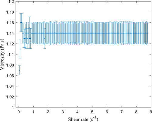
The rheology of the aqueous glycerol was measured using the Rheometer MCR 301. Figure 4 illustrates the average of three different tests for the viscosity measured against the shear rate at room temperature (20°C). The number of data points which were used to measure the viscosity by the Rheometer MCR 301 was 200 and the fix time was 1 s per point. The resulting flow curve is shown in Figure 4. It is clear that the aqueous glycerol solution behaves as Newtonian within the above mentioned shear rate range, the first point represents an apparatus artefact which has arisen in all the measurements.

Figure 4. Experimental data of viscosity vs. shear rate measured using Rheometer MCR 301 for aqueous glycerol ($\mu =1.14$ Pa·s).

3. Description of the mathematical models and numerical methods

3.1. Full model based on Navier-Stokes

The two-dimensional Navier-Stokes equations for an incompressible fluid can be defined as: (1) $\rho \left(\frac{\mathrm{\partial }u}{\mathrm{\partial }t}+u\frac{\mathrm{\partial }u}{\mathrm{\partial }x}+w\frac{\mathrm{\partial }u}{\mathrm{\partial }z}\right)=-\frac{\mathrm{\partial }p}{\mathrm{\partial }x}+\frac{\mathrm{\partial }}{\mathrm{\partial }x}\left(\mu \frac{\mathrm{\partial }u}{\mathrm{\partial }x}\right)+\frac{\mathrm{\partial }}{\mathrm{\partial }z}\left(\mu \frac{\mathrm{\partial }u}{\mathrm{\partial }z}\right)$(1) (2) $\rho \left(\frac{\mathrm{\partial }w}{\mathrm{\partial }t}+u\frac{\mathrm{\partial }w}{\mathrm{\partial }x}+w\frac{\mathrm{\partial }w}{\mathrm{\partial }z}\right)=-\frac{\mathrm{\partial }p}{\mathrm{\partial }z}+\frac{\mathrm{\partial }}{\mathrm{\partial }x}\left(\mu \frac{\mathrm{\partial }w}{\mathrm{\partial }x}\right)+\frac{\mathrm{\partial }}{\mathrm{\partial }z}\left(\mu \frac{\mathrm{\partial }w}{\mathrm{\partial }z}\right)-\rho g$(2) (3) $\frac{\mathrm{\partial }u}{\mathrm{\partial }x}+\frac{\mathrm{\partial }w}{\mathrm{\partial }z}=0$(3) where $(u,w)$ is the fluid velocity in the x and z direction respectively, while $\rho ,\mu$ and g are the density, viscosity and gravitational acceleration of the fluid.

The Navier–Stokes equations can be used to model Newtonian or non-Newtonian fluids depending on which rheological law is selected. We use the commercial Finite Element package COMSOL to solve the free surface flow. The ‘Laminar, Two-phase Flow, Moving Mesh’ interface of COMSOL was used to simulate the traversing fluid in the dam-break problem. The fully incompressible Navier–Stokes equations were solved in a domain that was deformed by the moving free surface of the fluid using the Arbitrary Lagrangian Eulerian (ALE) method. This method describes the mesh motion based on both the Lagrangian and Eulerian algorithms. In addition, the ALE method allows the mesh to conform to the evolving fluid domain as the free surface transforms over time. The Winslow mesh smoothing technique was used for propagating the mesh deformation throughout the domain. The initial computational domain was composed of two adjacent rectangles (representing the liquid levels in the tank), with dimensions as shown in Figure 5. The initial free surface of the fluid was composed of the top edges of the domain, and the sharp corners at $x=0\text{mm}$ were smoothed with 2-mm fillets, in order to avoid discontinuities of the free surface slope. The domain was tessellated with an unstructured mesh consisting of 1735 triangular elements (linear elements for velocity and pressure). The simulation was initialized with $u=w=0\text{m/s}$ and $p=0\mathrm{Pa}$ throughout the domain. The boundary conditions prescribed for the fluid phase were (i) no-slip on the base of the tank, (ii) Navier slip on the two end walls of the tank, and (iii) an external fluid interface for the free surface. Lastly, for the boundary conditions imposed on the moving mesh: (i) the base of the tank was fixed in the z-direction, (ii) the two ends of the tank were fixed in the x-direction, and (iii) no constraints were imposed on the mesh displacement at the free surface. A contact angle of 90° was imposed at the two end corners of the free surface. Moreover, a ramp function $\text{rm(}t)$ was used to ramp up the gravity body force to ease solution convergence. The ramp function was applied over $8.3\times {10}^{-3}\text{s}$, as shown in Figure 6.

Figure 5. Coordinate system.

Figure 6. Ramp function used in simulations.

In Figure 6, the slope gives an indication of the time required from the start of the simulation until it reaches the full gravity force. The gravity force $F_g$, which arose due to the volume of the fluid, is $F_g=-\rho g\text{rm(}t)$.

3.2. Model based on the lubrication approximation

The rheological model used to describe the non-Newtonian rheology of the fluid is the power-law model. The power-law model expresses viscosity in terms of the shear rate and has two parameters, the consistency factor (k, Pa.sⁿ) and the flow behaviour index (n, dimensionless). The rheology is described by the following relationship: (4) $\mu =k|\dot{\gamma }{|}^{n-\text{1}}$(4) For low Reynolds number and unidirectional flow Equations (1) and (2) can be approximated by: (5) $\frac{\mathrm{\partial }p}{\mathrm{\partial }x}=\frac{\mathrm{\partial }}{\mathrm{\partial }z}\left(\mu \frac{\mathrm{\partial }u}{\mathrm{\partial }z}\right)$(5) (6) $\frac{\mathrm{\partial }p}{\mathrm{\partial }z}=-\rho g$(6) Equation (5) can be integrated to obtain the following: $\mu \frac{\mathrm{\partial }u}{\mathrm{\partial }z}=\frac{\mathrm{\partial }p}{\mathrm{\partial }x}z+C_1$

The appropriate boundary condition should then be applied to find the value of the constant $C_1$. The free surface is shear-free, therefore: (7) $\frac{\mathrm{\partial }u}{\mathrm{\partial }z}=0\mathrm{on}z=h$(7) which leads to $C_1=-\left(\mathrm{\partial }p/\mathrm{\partial }x\right)h$.

Substituting in Equation (4) for the viscosity gives: (8) $k{\left|\frac{\mathrm{\partial }u}{\mathrm{\partial }z}\right|}^{n-1}\frac{\mathrm{\partial }u}{\mathrm{\partial }z}=\frac{\mathrm{\partial }p}{\mathrm{\partial }x}(z-h)$(8) The term $(z-h)$ is negative or zero because (0 < z < h) so the absolute value to this term leads to $(h-z)$. Therefore (9) $\left|\frac{\mathrm{\partial }u}{\mathrm{\partial }z}\right|={\left(\frac{1}{k}\right)}^{1/n}{\left|\frac{\mathrm{\partial }p}{\mathrm{\partial }x}\right|}^{1/n}\left(\right(h-z){)}^{1/n}$(9)

The term $\mathrm{\partial }u/\mathrm{\partial }z$ is always positive because $\mathrm{\partial }u/\mathrm{\partial }z$ is an increasing function of z. Integrating Equation (9) yields the following velocity profile: $u=\frac{-n}{n+1}{\left(\frac{1}{k}\right)}^{1/n}{\left|\frac{\mathrm{\partial }p}{\mathrm{\partial }x}\right|}^{1/n}\left(\right(h-z){)}^{(n+1)/n}+C_2$ But, since the no-slip boundary condition requires that (10) $u=w=0\mathrm{on}z=0,$(10) we obtain $C_2=\frac{n}{n+1}{\left(\frac{1}{k}\right)}^{1/n}{\left|\frac{\mathrm{\partial }p}{\mathrm{\partial }x}\right|}^{1/n}(h{)}^{(n+1)/n}$

Combining the above gives: (11) $u=\frac{n}{n+1}{\left(\frac{1}{k}\right)}^{1/n}{\left|\frac{\mathrm{\partial }p}{\mathrm{\partial }x}\right|}^{1/n}[(h{)}^{(n+1)/n}-(h-z{)}^{(n+1)/n}]$(11)

By applying the continuity equation for this plane flow, the following expression can obtained, which shows the relationship between the film thickness h and the flow rate Q. $\frac{\mathrm{\partial }h}{\mathrm{\partial }t}+\frac{\mathrm{\partial }Q}{\mathrm{\partial }x}=0$ $Q={\int }_0^{h}u\text{d}z$ (12) $\frac{\mathrm{\partial }h}{\mathrm{\partial }t}+\frac{\mathrm{\partial }}{\mathrm{\partial }x}{\int }_0^{h}u\text{d}z=0$(12)

Then, substituting Equation (11) into Equation (12) yields: (13) $\frac{\mathrm{\partial }h}{\mathrm{\partial }t}+\frac{n}{2n+1}{\left(\frac{1}{k}\right)}^{1/n}\frac{\mathrm{\partial }}{\mathrm{\partial }x}\left[{\left|\frac{\mathrm{\partial }p}{\mathrm{\partial }x}\right|}^{(1-n)/n}\frac{\mathrm{\partial }p}{\mathrm{\partial }x}{h}^{(2n+1)/n}\right]=0$(13) The free surface velocity can be obtained by substituting $z=h$ in Equation (11): (14) $u_s=\frac{n}{n+1}{\left(\frac{1}{k}\right)}^{1/n}{\left|\frac{\mathrm{\partial }p}{\mathrm{\partial }x}\right|}^{1/n}(h{)}^{(n+1)/n}$(14)

Integrating Equation (6) and applying the following boundary condition, we obtain an expression for the absolute pressure: (15) $p=-\sigma \frac{{\mathrm{\partial }}^{2}h}{\mathrm{\partial }{x}^2}\mathrm{on}z=h$(15) (16) $p=\rho g(h-z)-\sigma \frac{{\mathrm{\partial }}^{2}h}{\mathrm{\partial }{x}^2}$(16)

Equations (13) and (16) represent the lubrication approximation of the Navier-Stokes equations. The obtained differential equations are solved numerically using COMSOL Multiphysics. This software can solve a wide range of partial differential equations. Equations (13) and (16) were solved using the ‘Coefficient Form PDE’ interface of COMSOL. The lubrication approximation equations include two dependent variables, namely the fluid film thickness h and the film pressure p. To solve the lubrication approximation equations with COMSOL, Equations (13) and (16) are rewritten in the standard form solved by COMSOL: (17) $e_a\frac{{\mathrm{\partial }}^2\mathit{u}}{\mathrm{\partial }{t}^2}+d_a\frac{\mathrm{\partial }\mathit{u}}{\mathrm{\partial }t}+\mathrm{\nabla }\cdot (-c\mathrm{\nabla }\mathit{u}-\mathit{\alpha }\mathit{u}+\mathit{\gamma })+\mathit{\beta }\cdot \mathrm{\nabla }\mathit{u}+a\mathit{u}=\mathit{f},u=[h,p{]}^T.$(17)

In Equation (17), $e_a,d_a,c,\mathit{\alpha },\mathit{\gamma },\mathit{\beta },a$, and f are the coefficients which must be matched to Equations (13) and (16). The computational domain is a horizontal interval divided into quadratic elements; the total length was 0.916 m and the number of quadratic elements was 200. A zero gradient boundary condition is imposed at both ends ($\mathrm{\partial }p/\mathrm{\partial }x=0$ and $\mathrm{\partial }h/\mathrm{\partial }x=0$ at both $x=0$ and $x=L$). The initial free surface level for the dam-break problem is described by a smooth step function. A smooth function is used as a single-valued function with continuous derivatives is required for convergence. It is expected that the effect of this smoothing will be very minor and only apparent in the very early stages of the simulation. The initial value for p was zero. In both Equations (13) and (16) the coefficients of the dependent variables $h(x,t)$ and $p(x,t)$ were matched with the coefficients in Equation (17) as shown in Table 1.

Table 1. The coefficients of Equation (17) in COMSOL.

Coefficients of Equation (17)	Coefficients of $h(x,t)$ Equations (13)/(16)	Coefficients of $p(x,t)$ Equations (13)/(16)
$e_a$	0/0	0/0
$d_a$	1/0	0/0
$c$	0/−σ	0/0
$\alpha$	0/0	0/0
$\gamma$	${\displaystyle \frac{n}{2n+1}}{\left({\displaystyle \frac{\left|\mathrm{\partial }p/\mathrm{\partial }x\right|}{k}}\right)}^{1/n}\cdot h^{(2n+1)/n}$	0
$\beta$	0/0	0/0
$a$	0/− ρ g	0/1
$f$	0	0

The ability of COMSOL to accurately model such flows was demonstrated in [23]. Moreover, COMSOL has been validated as a numerical simulation tool for CFD, see for example [24] where the authors have demonstrated that COMSOL accurately models compressible flow in a shock tube. COMSOL uses the Backward Differentiation Formula (BDF) for the time-discretization which is an implicit integrator of variable order. That is, a high order is used when possible for accuracy, and a lower order will automatically be employed when necessary for stability.

3.3. Model validation

Neglecting the effect of surface tension, Equations (13) and (16) can be solved by using the method of similarity solutions described in [7,25]. The main steps of the derivation are shown below for clarity. Integrating the film thickness h from $x=0$ to the front position $x_N\left(t\right)$ gives the volume V which is invariant over time (18) $V={\int }_0^{x_N\left(t\right)}h\text{d}x$(18) The similarity solution of Equation (13) has the following form: (19) $h(x,t)={\xi }_N^{(n+1)/(n+2)}V{b}^{-1}{t}^{(-n)/(2n+3)}\psi \left(\chi \right),\chi =\frac{\xi }{{\xi }_N},$(19) where $\chi$ is the similarity variable, $\psi \left(\chi \right)$ a function yet to be determined, and $\xi$ and $b$ are defined as follows $\xi =x{b}^{-1}{t}^{(-n)/(2n+3)}$ (20) $b={\left[\frac{n}{2n+1}{\left(\frac{\rho g}{k}\right)}^{1/n}{V}^{(n+2)/n}\right]}^{n/(2n+3)}$(20)

Thus, $h(x,t)$ can be obtained from Equation (19). The position of the current front $x_N\left(t\right)$ can be determined according to (21) $x_N\left(t\right)={\xi }_{N}b{t}^{n/(2n+3)}$(21) It is clear that the position of the current front is a function of the rheological parameters, time and the volume of the flowing fluid [3,7]. Substituting the similarity solution (Equation (19)) into the partial differential Equation (13) yields an ordinary differential equation for the function $\psi \left(\chi \right)$ with the following solution (22) $\psi \left(\chi \right)={\left[\frac{n+2}{n+1}{\left(\frac{n}{2n+3}\right)}^n(1-{\chi }^{n+1})\right]}^{1/n+2}$(22) (23) $\begin{array}{rl}{\xi }_N& =\left[\frac{2}{n+1}{\left(\frac{n+2}{n+1}\right)}^{1/n+2}{\left(\frac{n}{2n+3}\right)}^{n/n+2}\right.\\ & \times {\left.\frac{\mathrm{\Gamma }(n+3/n+2)\mathrm{\Gamma }(1/n+1)}{\mathrm{\Gamma }\left(\right(n+3/n+2)+(1/n+1\left)\right)}\right]}^{-\left(\right(n+2\left)/\right(2n+3\left)\right)}\end{array}$(23) In order to verify the correct implementation of Equations (13) and (16) in COMSOL, the numerical solution is compared to the analytical one reported above. For both simulations the values of n, k and V were chosen to be 0.5, 20 Pa•sⁿ and 5 × 10⁻⁴ m³, respectively. The result are shown in Figure 7.

Figure 7. Profile of film thickness h for different times computed numerically (dashed lines) and analytically (full lines). (a) Numerical solution with 200 quadratic elements, (b) numerical solution 2000 quadratic elements.

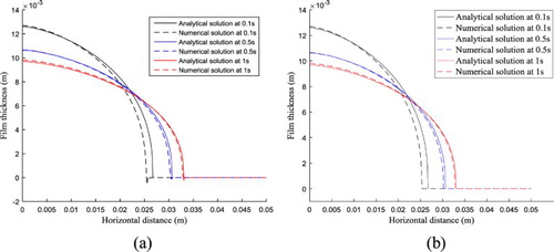
Figure 7 shows that the analytical and the numerical solution of the time dependent lubrication approximation are in good agreement. Small differences at early times can be attributed to the fact that a Dirac impulse function is assumed for the analytical solution, while a finite fluid depth H₀ has to be imposed as initial condition in COMSOL. Simulations were run on a coarse and fine mesh to check that the solution is mesh independent. Figure 7 confirms that that the difference between the coarse and fine mesh solutions is minimal.

4. Parameter identification

Parameter identification was also executed with COMSOL Multiphysics by performing an exhaustive parameter grid search and minimizing the mismatch between the measured and computed free surface velocity. To measure the mismatch, the following objective function (OF) was defined for N time periods in the experimental data: (24) $OF(k,n)=\sum _{i=1}^{N}0.5{\int }_0^L{\left(u_c\right(x,t=i\mathrm{\Delta }t)-{u_m}_{(}x,t=i\mathrm{\Delta }t))}^2\text{d}x$(24) where $u_m$ is the measured free surface velocity obtained from the experiment, while $u_c$ is the computed velocity from the lubrication approximation, i.e. Equations (13) and (16). The rheological parameters which minimize the objective function are unknown. Consequently, wide ranges of n $(0<n\le 2)$ and k $(0<k\le 50)$ were used to calculate the objective function and to generate the contour map of the objective function in the parameter space. The rheological parameters of the used fluid should correspond to the minimum of the objective function. The difference between the experimental and the numerical data is minimal at this point.

4.1. Identification with perfect synthetic data

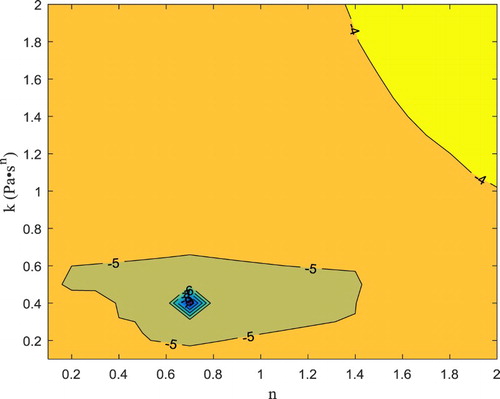
In order to test the proposed methodology, synthetic experimental data were produced by running COMSOL with k = 0.4 Pa•sⁿ and n = 0.7 using the lubrication approximation solver and generating a series of free surface velocities using Equation (14). This correspond to a fluid with a shear thinning rheology. The exhaustive grid search was then undertaken to check that the minimum of the objective function occurred at the correct values of n and k. The following figure represents contour lines of the log values of the objective function.

From the above Figures, the minimum value of the objective function is (1.06 × 10⁻¹¹) at n = 0.7 and k = 0.4 Pa•sⁿ. Beyond the parameter space shown in Figure 8, the objective function increases monotonically as far as we have tested. The above result suggests there exists a unique minimum which means that the identification problem is well-posed.

Figure 8. Contour lines for the log values of the objective function with respect to the rheological parameters obtained from the exhaustive grid search with synthetic data. The minimum is correctly located at k = 0.4 ± 0.1 Pa•sⁿ and n = 0.7 ± 0.1, as expected.

In addition, another synthetic experimental dataset was produced by running COMSOL with k = 0.5 Pa•sⁿ and n = 1.5 using the two-dimensional Navier-Stokes solver. This correspond to a fluid with a shear thickening rheology. The results of the parameter identification are shown in Figure 9. The results show again the existence of a global minimum and the successful identification of the parameters since the values n = 1.5 and k = 0.5 Pa•sⁿ were recovered.

Figure 9. Contour lines for the log values of the objective function as a function of the rheological parameters obtained from the exhaustive grid search with synthetic data obtained from the two-dimensional Navier-Stokes solver. The minimum is correctly located at k = 0.5 ± 0.1 Pa•sⁿ and n = 1.5 ± 0.1.

With the parameters now identified, it is interesting to compare the free surface profiles obtained from the two-dimensional Navier-Stokes solver and from the lubrication approximation, see Figure 10.

Figure 10. Comparison between film thickness profile computed using the two-dimensional Navier-Stokes solver and the lubrication approximation at three different time periods, namely 0.5 s, 5 s and 10 s respectively (k = 0.5 ± 0.1 Pa•sⁿ and n = 1.5 ± 0.1).

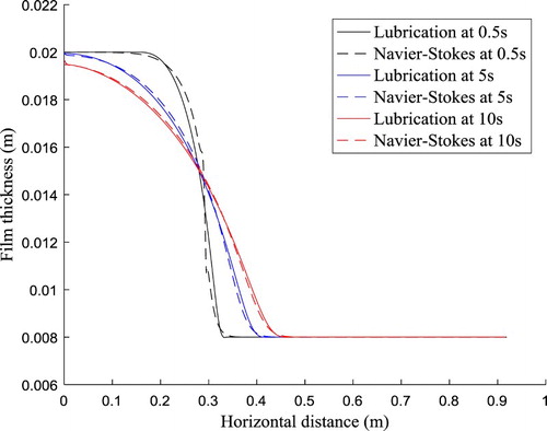
Figure 10 shows film thickness as a function of the horizontal distance along the centreline of the tank at different time periods. The good agreement between the Navier-Stokes and lubrication approximation confirms that in that particular regime, the hypothesis underlying the lubrication approximation are valid.

4.2. Identification with noisy synthetic data

The previous results have illustrated that the proposed strategy is able to reconstruct rheological parameters from an ideal data set for the free surface velocity. However, experimental data is typically affected by noise. Before attempting to use true experimental data, it is necessary to better understand how sensitive the reconstruction algorithm is to the presence of noise as done in [26,27]. Artificial noise is added to the synthetic data of Section 4.1 and the parameter identification process is repeated. The OF in Equation (24) is rewritten to include the noise component as follows: (25) $OF(k,n)=\sum _{i=1}^{N}0.5{\int }_0^L{\left(u_c\right(x,t=i\mathrm{\Delta }t)-(u_m(x,t=i\mathrm{\Delta }t)+e\left)\right)}^2\text{d}x$(25) The amount of noise in Equation (25) depends on the maximum and the minimum value of the synthetic free surface velocity as well as the percentage of the noise and was calculated using Equation (26). (26) $e=\alpha (u_{max}-u_{min})E$(26) where e is the noise, $u_{\max }$ and $u_{\min }$ represent the maximum and the minimum values of the free surface velocity respectively, and α the percentage of noise. E is a number with values randomly distributed between −1 and +1. Results have confirmed that the identified values of the rheological parameters remain the same even for large values of the added noise. For 40% added noise, the reconstructed rheological parameters are n = 0.7 and k = 0.4 Pa•sⁿ.

Figure 11 shows contour plots of the objective function in the parameter space for two cases, the first is without added noise (on the left-hand-side) and the second is with 40% added noise (on the right-hand side). It is worth noting that the presence of noise widens the valley around the minimum.

Figure 11. Contour maps of the log values of the objective function as a function of the rheological parameters without noise (left-hand-side) and with 40% added noise (right-hand-side).

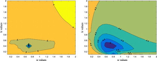
From Figure 11, there is no difference in the flow behaviour index and only a minor difference in the identified consistency factor. The absolute error is 0.05 Pa•sⁿ, while the relative error percentage is 12.5%.

4.3. Identification with experimental data

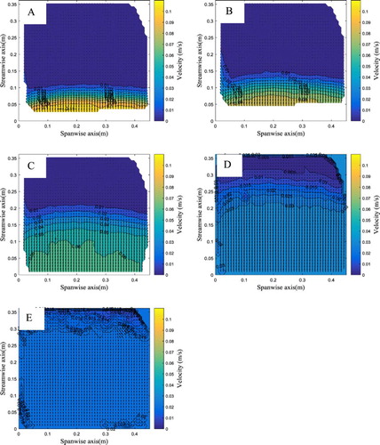
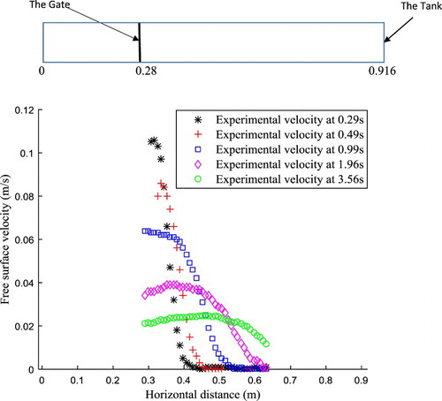
Five time periods were chosen from the experimental data for comparison with the simulation, namely 0.29 s, 0.49 s, 0.99 s, 1.96 s and 3.56 s, respectively. After the 3.56 s the levelling is near complete and the velocity fluctuations are below 0.02 m/s and therefore the velocity signal becomes unreliable. The velocity vector field related to these time periods is shown in Figure 12.

Figure 12. Velocity vector field for a five different time periods, namely (A) 0.29 s, (B) 0.49 s, (C) 0.99 s, (D) 1.96 s and (E) 3.56 s.

Using the viscosity data from Figure 4 ($n=1$ and $k=1.14$ Pa·sⁿ), the velocity magnitude, and film thickness measured experimentally, we can estimate the important dimensionless groups like the Reynolds number $Re=Uh\rho /\mu$, the Froude number $\text{Fr}=U/\sqrt{\text{gh}}$ and the Weber number $We=\rho h{U}^2/\sigma$. The Reynolds number represents the ratio of the fluid inertia to the viscous forces, the Froude number represents the ratio of the flow inertia to the gravitational force, while the Weber number represents the ratio of inertia to the surface tension. In the present case, it was found that $Re=1.94$, $\text{Fr}=0.27$ and $We=3.92$ for the used aqueous glycerol with $\rho =1257\text{kg/}{\text{m}}^3$, $U=0.11\text{m/s}$, $h=0.016\text{m}$, $\mu =1.14\text{Pa}\text{.s}$ and $\sigma =0.062\text{N/m}$, which implies that the flow is laminar with low inertia hence justifying the lubrication approximation.

From Figure 12, it is clear that the free surface velocity is maximum at the gate (zero on the Y axis) and decreases with the distance from the gate, as expected. The velocity profiles taken from the centreline of the tank are shown in Figure 13 (the velocity profile is computed by averaging over a 2.7 cm-wide band around the centreline of the tank. Over this region, the velocity was assumed to be unaffected the frictional effects of the walls).

Figure 13. Velocity distribution data (average) of aqueous glycerol along the tank centreline for five time periods, namely 0.29 s. 0.49 s, 0.99 s, 1.96 s and 3.56 s, respectively.

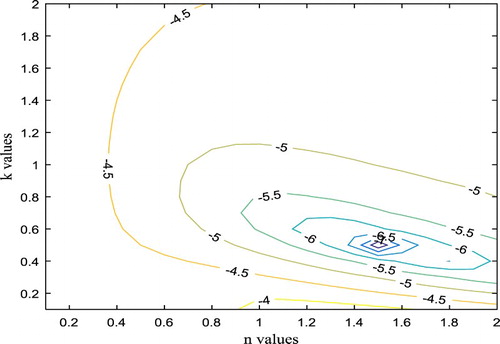
Having validated the parameter identification algorithm with synthetic data, the process is now applied to the experimental data. From the exhaustive parameter grid search, it was found that the objective function has a minimum at n = 1.0 ± 0.1 & k = 1.3 ± 0.1 Pa•sⁿ for the aqueous glycerol as shown in Figure 14.

Figure 14. Contour lines for the log values of the objective function with respect to the rheological parameters for aqueous glycerol. The minimum occurs at k = 1.3 ± 0.1 Pa•sⁿ and n = 1.0 ± 0.1.

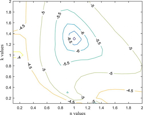
Again, the landscape of the objective function confirms the uniqueness of the solution since there is a unique minimum and the objective function increases for points which are more and more distant in the parameter space.

After evaluating the rheological parameters, it is easy to calculate the values of the computed free surface velocity obtained from Equation (14). Figure 15 shows a comparison of the free surface velocity measured experimentally along the tank centreline and that computed for the optimal values of n and k at five different time periods.

Figure 15. Comparison between the experimental free surface velocity (crosses), the computed velocity based on the lubrication approximation equation (solid line) and the computed velocity based on the Navier–Stokes equation (dashed line) at a five different time periods, (a) 0.29 s, (b) 0.49 s, (c) 0.99 s, (d) 1.96 s and (e) 3.56 s.

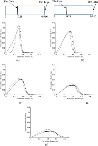
One of the first things to note is that all the velocity profiles are in good agreement. The discrepancy is larger for the latest time. One possible explanation is the presence of the side wall which invalidate the plane flow assumption. Initially the effect of the wall on the velocity is minimal and the particle trajectories are straight. However, these paths become curved with increasing time as shown in Figure 3. The computed velocity based on the lubrication approximation and that based on the Navier–Stokes equations are close, which means that inertia does not have a significant effect in this parameter range.

The value of the viscosity of the aqueous glycerol solution, which was measured by the rheometer was (1.14 Pa.s), while the viscosity which is obtained from the identification is (1.3 Pa.s). Consequently, the absolute error is 0.16 Pa.s, while the relative error percentage is 14%. For reference, the error values are less than that calculated in [7]. The cause of this error is likely due to the experimental system. One limitation of the experiment is that a single camera can only capture the two in-plane components of the velocity vector, leaving the out-of-plane velocity component unresolved. Therefore, vertical movement in the wave cannot be accounted for. Another error is the measurement of the fluid level had an accuracy of 0.1 mm and the measurement of the tank horizontally had an accuracy of 1 mm per 1 m.

5. Conclusion

We have demonstrated in this work that the free surface velocity can be used as a proxy to identify the rheology of a fluid. The main idea is to find the optimal rheological parameters which minimize the mismatch between measured and simulated data. In order to test this conceptual idea, we considered the dam-break flow problem. Free surface velocity maps were generated by tracking the trajectories of buoyant beads seeded at the free surface of the flow and using PTV. Two modelling approaches were implemented in COMSOL Multiphysics to simulate the flow: the first is based on the full Navier-Stokes equations with a moving mesh to capture the evolving domain and the second is based on the lubrication approximation. The latter is used for the identification procedure because the simulation time is orders of magnitude smaller enabling a timely sweep of the parameter space. Of course, this approach is only applicable if the underlying assumptions which justify the lubrication approximation are satisfied which is the case in the flows considered here. Using the full Navier-Stokes model is possible but the computational cost would be prohibitive. When plotting maps of the objective function which provides a measure of the mismatch between measured and simulated data, it was clear that a unique minimum in the parameter space could be identified confirming the hypothesis that the rheology can be inferred. The identification was tested on ideal synthetic data generated by running the models forward, noisy synthetic data, and true experimental data. In all cases a unique minimum of the objective function in the parameter space was identified. The process was shown to be robust since the addition of significant noise on the data did not prevent a reasonable identification of the rheological parameters.

On the other hand, the proposed method has limitations worth acknowledging. Firstly, the method needs to assume a rheological law. The power-law rheology is the one which requires the least parameters (only two parameters). More complex rheologies are possible but they require more parameters making the identification more difficult, potentially leading to an ill-posed problem. Secondly, the flow is assumed to be planar. The ability to remove this requirement would certainly broaden the range of potential applications. The limit will however always be computational time. Hundreds of simulations are necessary to canvass the parameter space so every single simulation needs to be fast enough. This leads on the another possible area of improvement. We used a ‘brute force’ identification technique by systematically surveying the parameter space. Much more efficient algorithms exist to make the procedure much more efficient.

Notwithstanding the above limitations, the proposed technique could prove invaluable in situations where the fluid rheology cannot be measured using standard rheometry techniques because the fluid sample is extremely hot (lava), dangerous (nuclear wastes), in too small a quantity (aerosol particles), or inaccessible (remotely observed flows on other planets).

Acknowledgements

The kind support of Lidia Motoi, Louisiane Devaud and Deborah Le Corre-Bordes with the rheometer is gratefully acknowledged.

Disclosure statement

No potential conflict of interest was reported by the authors.

References

- Sellier M. Inverse problems in free surface flows: a review. Acta Mech. 2016;227(3):913–935.
- Foit J. Spreading under variable viscosity and time-dependent boundary conditions: estimate of viscosity from spreading experiments. Nucl Eng Des. 2004;227(2):239–253.
- Longo S, Di Federico V, Archetti R, et al. On the axisymmetric spreading of non-Newtonian power-law gravity currents of time-dependent volume: an experimental and theoretical investigation focused on the inference of rheological parameters. J Nonnewton Fluid Mech. 2013;201:69–79.
- Longo S, Di Federico V, Chiapponi L. Non-Newtonian power-law gravity currents propagating in confining boundaries. Environ Fluid Mech. 2015;15(3):515–535.
- Gratton J, Minotti F, Mahajan SM. Theory of creeping gravity currents of a non-Newtonian liquid. Phys Rev E. 1999;60(6):6960–6967.
- Starov VM, Tyatyushkin AN, Velarde MG, et al. Spreading of non-Newtonian liquids over solid substrates. J Colloid Interface Sci. 2003;257(2):284–290.
- Sayag R, Worster MG. Axisymmetric gravity currents of power-law fluids over a rigid horizontal surface. J Fluid Mech. 2013;716:R5.
- Perona P. Bostwick degree and rheological properties: an up-to-date viewpoint. Appl Rheol . 2005;15 (EPFL-ARTICLE-149755):218–229.
- Piau J-M, Debiane K. Consistometers rheometry of power-law viscous fluids. J Nonnewton Fluid Mech. 2005;127(2):213–224.
- Balmforth NJ, Craster RV, Perona P, et al. Viscoplastic dam breaks and the Bostwick consistometer. J Nonnewton Fluid Mech. 2007;142(1):63–78.
- Renbaum-Wolff L, Grayson JW, Bateman AP, et al. Viscosity of -pinene secondary organic material and implications for particle growth and reactivity. Proc Natl Acad Sci U S A. 2013;110(20):8014–8019.
- Grayson JW, Song M, Sellier M, et al. Validation of the poke-flow technique combined with simulations of fluid flow for determining viscosities in samples with small volumes and high viscosities. Atmos Meas Tech. 2015;8(6):2463–2472.
- Sellier M, Grayson JW, Renbaum-Wolff L, et al. Estimating the viscosity of a highly viscous liquid droplet through the relaxation time of a dry spot. J Rheol (N Y N Y). 2015;59(3):733–750.
- Eggers J. Nonlinear dynamics and breakup of free-surface flows. Rev Mod Phys. 1997;69(3):865–929.
- Bazilevsky AV, Entov VM, Rozhkov AN. Liquid filament microrheometer and some of its applications. In: Third European Rheology Conference and Golden Jubilee Meeting of the British Society of Rheology. Dordrecht: Springer; 1990. p. 41–43.
- McKinley GH, Tripathi A. How to extract the Newtonian viscosity from capillary breakup measurements in a filament rheometer. J Rheol (N Y N Y). 2000;44(3):653–670.
- Matta JE, Tytus RP. Liquid stretching using a falling cylinder. J Nonnewton Fluid Mech. 1990;35(2):215–229.
- Anna SL, Rogers C, McKinley GH. On controlling the kinematics of a filament stretching rheometer using a real-time active control mechanism. J Nonnewton Fluid Mech. 1999;87(2):307–335.
- Figliuzzi B, Jeulin D, Lemaître A, et al. Rheology of thin films from flow observations. Exp Fluids. 2012;53(5):1289–1299.
- Moran K, Yeung A. Determining bitumen viscosity through drop shape recovery. Can J Chem Eng. 2004;82(4):813–820.
- Martin N, Monnier J. Inverse rheometry and basal properties inference for pseudoplastic geophysical flows. Eur J Mech B Fluids. 2015;50:110–126.
- Nokes R. Streams v2.03 system theory and design. Christchurch: University of Canterbury; 2014.
- Morris S, Sellier M, Behadili ARA. Comparison of Lubrication Approximation and Navier-Stokes Solutions for Dam-Break Flows in Thin Films. arXiv preprint arXiv:1708.00976, 2017.
- Darrell WP, Xiuling W. Benchmarking COMSOL 3.5a - CFD problems. COMSOL CONFERENCE; 2009; Boston, MA, USA.
- Huppert HE. The propagation of two-dimensional and axisymmetric viscous gravity currents over a rigid horizontal surface. J Fluid Mech. 1982;121:43–58.
- Heining C, Sellier M. Direct reconstruction of three-dimensional glacier bedrock and surface elevation from free surface velocity. AIMS Geosci. 2016;2:45–63.
- Sellier M, Panda S. Unraveling surfactant transport on a thin liquid film. Wave Motion. 2017;70:183–194.