Stable explicit stepwise marching scheme in ill-posed time-reversed 2D Burgers' equation

ABSTRACT

This paper constructs an unconditionally stable explicit difference scheme, marching backward in time, that can solve a limited, but important class of time-reversed 2D Burgers' initial value problems. Stability is achieved by applying a compensating smoothing operator at each time step to quench the instability. This leads to a distortion away from the true solution. However, in many interesting cases, the cumulative error is sufficiently small to allow for useful results. Effective smoothing operators based on $(-\mathrm{\Delta }{)}^p$, with real p>2, can be efficiently synthesized using FFT algorithms, and this may be feasible even in non-rectangular regions. Similar stabilizing techniques were successfully applied in other ill-posed evolution equations. The analysis of numerical stability is restricted to a related linear problem. However, extensive numerical experiments indicate that such linear stability results remain valid when the explicit scheme is applied to a significant class of time-reversed nonlinear 2D Burgers' initial value problems. As illustrative examples, the paper uses fictitiously blurred $256\times 256$ pixel images, obtained by using sharp images as initial values in well-posed, forward 2D Burgers' equations. Such images are associated with highly irregular underlying intensity data that can seriously challenge ill-posed reconstruction procedures. The stabilized explicit scheme, applied to the time-reversed 2D Burgers' equation, is then used to deblur these images. Examples involving simpler data are also studied. Successful recovery from severely distorted data is shown to be possible, even at high Reynolds numbers.

KEYWORDS:

• 2D viscous Burgers' equation backward in time
• high Reynolds numbers
• stabilized explicit marching difference scheme
• numerical experiments

AMS SUBJECT CLASSIFICATIONS:

• 35K59
• 35Q30
• 35R25
• 65M12
• 65M30

1. Introduction

Following the 1951 seminal paper by Cole [1], a large literature on the 2D Burgers' equation has developed, spawned by significant applications in science and engineering. Numerous references may be found in recent papers [2–7]. As is often stressed, the 2D Burgers' coupled system is a useful simplification of the 2D incompressible Navier-Stokes equations, providing valuable insight into the behaviour of complex flows, together with the expected behaviour of possible numerical methods for computing such flows. Accordingly, numerical methods for the well-posed forward Burgers' initial value problem have been actively investigated.

On the other hand, very little seems known about possible numerical computation of the ill-posed time-reversed 2D Burgers' equation. The backward problem is of considerable interest, as it may enable computation of initial conditions that can produce desired flow patterns, as well as reconstructing the genesis of undesired flows. Such inverse design problems are actively being studied for the 1D Burgers' equation [8–10]. The inverse Burgers' problem also plays an important role in studies of data assimilation for nonlinear geophysical fluid dynamics [11–14]. Error estimates of logarithmic convexity type have been obtained for backward recovery in the 1D problem [15, 16], but are not yet known in the 2D Burgers' problem. For the Navier-Stokes equations, backward error estimates are given in [17, 18]. Further information about ill-posed continuation in partial differential equations may be found in [19–22].

The present self-contained paper constructs an unconditionally stable explicit difference scheme, marching backward in time, that can solve an important but limited class of time-reversed 2D Burgers' initial value problems. Stability is achieved by applying a compensating smoothing operator at each time step to quench the instability. Eventually, this leads to a distortion away from the true solution. However, in many interesting cases, the cumulative effect of these errors is sufficiently small to allow for useful results. Effective smoothing operators based on $(-\mathrm{\Delta }{)}^p$, with real p>2, can be efficiently synthesized using FFT algorithms. Similar stabilizing techniques were successfully applied in other ill-posed evolution equations, [23–26]. As was the case in these papers, the analysis of numerical stability given in Sections 3 and 4 below, is restricted to a related linear problem. However, extensive numerical experiments indicate that these linear stability results remain valid when the explicit scheme is applied to a significant class of time-reversed nonlinear Burgers' initial value problems.

Following [1], we define the Reynolds number RE as follows (1) $\mathrm{RE}=\left(\sqrt{A}/\nu \right)U_{max}$(1) where A is the area of the flow domain, ν is the kinematic viscosity and $U_{max}$ is the maximum value of the initial velocity. In many numerical experiments on the well-posed forward 2D Burgers' equation, the objective is to demonstrate accurate calculation of an exact solution, known analytically together with its specific initial and time-dependent boundary values. Typically, with $100\le \mathrm{RE}\le 1000$, computations are carried out up to some fixed time $T_{max}\ge 1$. In the present time-reversed context, where only approximate values are generally available at some positive time $T_{max}$, the objective is to demonstrate useful backward reconstruction from noisy data. As is well known, there is a necessary uncertainty in ill-posed backward recovery from imprecise data at $T_{max}$. For the 1D Burgers' equation, the error estimates at t=0 given in [15, 16], contain a factor $K=\exp \{\mathrm{RE}\times T_{max}\}$. For the Navier-Stokes equations, the corresponding uncertainty may be significantly larger [17, 18]. Taken together, these results indicate that successful backward recovery in the 2D Burgers' equation, with $100\le \mathrm{RE}\le 1000$, may not be feasible unless $T_{max}\ll 1$.

In Section 5 below, three instructive numerical experiments are discussed. In these experiments, the solutions have the value zero on the domain boundary. Interesting initial values are propagated forward up to a time $T_{max}\ll 1$, by numerically solving the well-posed forward 2D Burgers' equation. Despite the small value of $T_{max}$, considerable distortion of the initial values occurs. These limited precision numerical values are then used as input data at $T_{max}$, for the backward computation with the stabilized explicit scheme. In the first experiment, relatively simple data are used, involving two Gaussians on the unit square, and $T_{max}=2.5\times {10}^{-3}$ with $\mathrm{RE}=50,000$. The second experiment involves images on the unit square, defined by highly non-smooth intensity data. Here, $T_{max}=2.5\times {10}^{-4}$ and $\mathrm{RE}=3400$. The last experiment, with $T_{max}=2.5\times {10}^{-4}$ and $\mathrm{RE}=2500$, involves non-smooth image data in an elliptical region.

2. 2D Burgers' equation

Let Ω be the unit square in $R^2$ with boundary $\mathrm{\partial \Omega }$. Let $<,>$ and $\parallel {\parallel }_2$, respectively, denote the scalar product and norm on ${\mathcal{L}}^2\left(\mathrm{\Omega }\right)$. With $\nu >0$ the kinematic viscosity, we consider the following 2D Burgers' system for $(x,y)\in \mathrm{\Omega },$ (2) $\begin{array}{rl}{u}_t& =L_{1}u\equiv \nu \mathrm{\Delta }u-u{u}_x-v{u}_y,0<t\le T_{max},\\ v_t& =L_{2}v\equiv \nu \mathrm{\Delta }v-u{v}_x-v{v}_y,0<t\le T_{max},\end{array}$(2) together with periodic boundary conditions on $\mathrm{\partial \Omega }$, and the initial values (3) $u(x,y,0)=u_0(x,y),v(x,y,0)=v_0(x,y),(x,y)\in \mathrm{\Omega }.$(3) The well-posed forward initial value problem in Equation (2(2) $\begin{array}{rl}{u}_t& =L_{1}u\equiv \nu \mathrm{\Delta }u-u{u}_x-v{u}_y,0<t\le T_{max},\\ v_t& =L_{2}v\equiv \nu \mathrm{\Delta }v-u{v}_x-v{v}_y,0<t\le T_{max},\end{array}$(2) ) becomes ill-posed if the time direction is reversed, and one wishes to recover $u(x,y,0)),v(x,y,0)$, from given approximate values for $u(x,y,T_{max}),v(x,y,T_{max})$. We contemplate such time-reversed computations by allowing for possible negative time steps $\mathrm{\Delta }t$ in the explicit time-marching finite difference scheme described below. With a given positive integer N, let $|\mathrm{\Delta }t|=T_{max}/(N+1)$ be the time step magnitude, and let ${\tilde{u}}^n(x,y)\equiv \tilde{u}(x,y,n\mathrm{\Delta }t),n=0,1,\dots ,N+1$, denote the intended approximation to $u(x,y,n\mathrm{\Delta }t)$, and likewise for ${\tilde{v}}^n(x,y)$. It is helpful to consider Fourier series expansions for ${\tilde{u}}^n(x,y),{\tilde{v}}^n(x,y)$, on the unit square Ω, (4) ${\tilde{u}}^n(x,y)=\sum _{j,k=-\mathrm{\infty }}^{\mathrm{\infty }}{\tilde{u}}_{j,k}^n\exp \left\{2\pi i\right(jx+ky\left)\right\},$(4) with Fourier coefficients $\left\{{\tilde{u}}_{j,k}^n\right\}$ given by (5) ${\tilde{u}}_{j,k}^n={\int }_{\mathrm{\Omega }}{\tilde{u}}^n(x,y)\exp \{-2\pi i(jx+ky\left)\right\}\mathrm{d}x\mathrm{d}y,$(5) and similarly for ${\tilde{v}}^n(x,y)$. With given fixed $\omega >0$ and p>1, define ${\lambda }_{j,k},{\sigma }_{j,k}$, as follows (6) ${\lambda }_{j,k}=4{\pi }^2\nu (j^2+k^2),{\sigma }_{j,k}=\exp \{-2\omega |\mathrm{\Delta }t|{\lambda }_{j,k}^p\}.$(6) For any $f(x,y)\in {\mathcal{L}}^2\left(\mathrm{\Omega }\right)$, let $\left\{f_{j,k}\right\}$ be its Fourier coefficients as in Equation (5(5) ${\tilde{u}}_{j,k}^n={\int }_{\mathrm{\Omega }}{\tilde{u}}^n(x,y)\exp \{-2\pi i(jx+ky\left)\right\}\mathrm{d}x\mathrm{d}y,$(5) ). Using Equation (6(6) ${\lambda }_{j,k}=4{\pi }^2\nu (j^2+k^2),{\sigma }_{j,k}=\exp \{-2\omega |\mathrm{\Delta }t|{\lambda }_{j,k}^p\}.$(6) ), define the linear operators P and S as follows (7) $\begin{array}{rl}Pf& =\sum _{j,k=-\mathrm{\infty }}^{\mathrm{\infty }}{\lambda }_{j,k}^p{f}_{j,k}\exp \left\{2\pi i\right(jx+ky\left)\right\},\mathrm{\forall }f\in {\mathcal{L}}^2\left(\mathrm{\Omega }\right),\\ Sf& =\sum _{j,k=-\mathrm{\infty }}^{\mathrm{\infty }}{\sigma }_{j,k}{f}_{j,k}\exp \left\{2\pi i\right(jx+ky\left)\right\},\mathrm{\forall }f\in {\mathcal{L}}^2\left(\mathrm{\Omega }\right).\end{array}$(7) As in [23–26], the operator S is used as a stabilizing smoothing operator at each time step, in the following explicit time-marching finite difference scheme for the system in Equation (2(2) $\begin{array}{rl}{u}_t& =L_{1}u\equiv \nu \mathrm{\Delta }u-u{u}_x-v{u}_y,0<t\le T_{max},\\ v_t& =L_{2}v\equiv \nu \mathrm{\Delta }v-u{v}_x-v{v}_y,0<t\le T_{max},\end{array}$(2) ), in which only the time variable is discretized, while the space variables remain continuous, (8) $\begin{array}{rl}{\tilde{u}}^{n+1}& =S{\tilde{u}}^n+\mathrm{\Delta }tS{L}_1{\tilde{u}}^n,\\ {\tilde{v}}^{n+1}& =S{\tilde{v}}^n+\mathrm{\Delta }tS{L}_2{\tilde{v}}^n,n=0,1,\dots ,N.\end{array}$(8) The analyses presented in Sections 3 and 4 below are relevant to the above semi-discrete problem. In Section 5, where actual numerical computations are discussed, the space variables are also discretized, and FFT algorithms are used to synthesize the smoothing operator S.

3. Fourier stability analysis in linearized problem

As in [23–26], useful insight into the behaviour of the nonlinear scheme in Equation (8(8) $\begin{array}{rl}{\tilde{u}}^{n+1}& =S{\tilde{u}}^n+\mathrm{\Delta }tS{L}_1{\tilde{u}}^n,\\ {\tilde{v}}^{n+1}& =S{\tilde{v}}^n+\mathrm{\Delta }tS{L}_2{\tilde{v}}^n,n=0,1,\dots ,N.\end{array}$(8) ), can be gained by analysing a related linear problem with constant coefficients. With positive constants $a,b,$ consider the initial value problem on the unit square Ω, (9) $\begin{array}{rl}{u}_t& =Lu\equiv \nu \mathrm{\Delta }u-a{u}_x-b{u}_y,0<t\le T_{max},\\ u(x,y,0)& =u_0(x,y),\end{array}$(9) together with periodic boundary conditions on $\mathrm{\partial \Omega }$. Unlike the case in Equation (8(8) $\begin{array}{rl}{\tilde{u}}^{n+1}& =S{\tilde{u}}^n+\mathrm{\Delta }tS{L}_1{\tilde{u}}^n,\\ {\tilde{v}}^{n+1}& =S{\tilde{v}}^n+\mathrm{\Delta }tS{L}_2{\tilde{v}}^n,n=0,1,\dots ,N.\end{array}$(8) ), the stabilized marching scheme (10) ${\tilde{u}}^{n+1}=S{\tilde{u}}^n+\mathrm{\Delta }tSL{\tilde{u}}^n,n=0,1,\dots ,N,$(10) with the linear operator L, is susceptible to Fourier analysis. If $L{\tilde{u}}^n=f^n(x,y)$, then the Fourier coefficients $\left\{f_{j,k}^n\right\}$ satisfy $f_{j,k}^n=g_{j,k}{\tilde{u}}_{j,k}^n$, where, with ${\lambda }_{j,k}$ as in Equation (6(6) ${\lambda }_{j,k}=4{\pi }^2\nu (j^2+k^2),{\sigma }_{j,k}=\exp \{-2\omega |\mathrm{\Delta }t|{\lambda }_{j,k}^p\}.$(6) ), (11) $g_{j,k}=-\{{\lambda }_{j,k}+2\pi i(aj+bk\left)\right\}.$(11) Let R be the linear operator $R=S+\mathrm{\Delta }tSL$. Then, (12) $\begin{array}{rl}{\tilde{u}}^{n+1}& =R{\tilde{u}}^n\equiv \sum _{j,k=-\mathrm{\infty }}^{\mathrm{\infty }}{\tilde{u}}_{j,k}^n\{1+\mathrm{\Delta }t{g}_{j,k}\}{\sigma }_{j,k},\\ \parallel {\tilde{u}}^{n+1}{\parallel }_2^2& =\parallel R{\tilde{u}}^n{\parallel }_2^2\le \sum _{j,k=-\mathrm{\infty }}^{\mathrm{\infty }}|{\tilde{u}}_{j,k}^n{|}^2\{1+|\mathrm{\Delta }t||g_{j,k}|{\}}^2{\sigma }_{j,k}^2,\end{array}$(12) on using Parseval's formula.

Lemma 3.1

Let ${\lambda }_{j,k},{\sigma }_{j,k},$ be as in Equation (6(6) ${\lambda }_{j,k}=4{\pi }^2\nu (j^2+k^2),{\sigma }_{j,k}=\exp \{-2\omega |\mathrm{\Delta }t|{\lambda }_{j,k}^p\}.$(6) ), and let $g_{j,k}$ be as in Equation (11(11) $g_{j,k}=-\{{\lambda }_{j,k}+2\pi i(aj+bk\left)\right\}.$(11) ). Choose a positive integer J such that if ${\lambda }_J=4{\pi }^2\nu J,$ we have (13) $\underset{(j^2+k^2)\le J}{max}\left\{|g_{j,k}|\right\}\le 2{\lambda }_J,|g_{j,k}|\le 2{\lambda }_{j,k},\mathrm{\forall }(j^2+k^2)>J.$(13) With $p>1,$ choose $\omega \ge ({\lambda }_J{)}^{1-p}$ in Equation (6(6) ${\lambda }_{j,k}=4{\pi }^2\nu (j^2+k^2),{\sigma }_{j,k}=\exp \{-2\omega |\mathrm{\Delta }t|{\lambda }_{j,k}^p\}.$(6) ). Then, (14) ${\sigma }_{j,k}\left(1+|\mathrm{\Delta }t||g_{j,k}|\right)\le 1+2|\mathrm{\Delta }t|{\lambda }_J.$(14) Hence, from Equation (12(12) $\begin{array}{rl}{\tilde{u}}^{n+1}& =R{\tilde{u}}^n\equiv \sum _{j,k=-\mathrm{\infty }}^{\mathrm{\infty }}{\tilde{u}}_{j,k}^n\{1+\mathrm{\Delta }t{g}_{j,k}\}{\sigma }_{j,k},\\ \parallel {\tilde{u}}^{n+1}{\parallel }_2^2& =\parallel R{\tilde{u}}^n{\parallel }_2^2\le \sum _{j,k=-\mathrm{\infty }}^{\mathrm{\infty }}|{\tilde{u}}_{j,k}^n{|}^2\{1+|\mathrm{\Delta }t||g_{j,k}|{\}}^2{\sigma }_{j,k}^2,\end{array}$(12) ), $\parallel R{\parallel }_2\le 1+2|\mathrm{\Delta }t|{\lambda }_J,$ and (15) $\parallel {\tilde{u}}^n{\parallel }_2=\parallel R^n{u}_0{\parallel }_2\le \exp \left\{2n|\mathrm{\Delta }t|{\lambda }_J\right\}\parallel u_0{\parallel }_2,n=1,2,\dots ,N+1.$(15) Therefore, with this choice of $(\omega ,p),$ the explicit linear marching scheme in Equation (10(10) ${\tilde{u}}^{n+1}=S{\tilde{u}}^n+\mathrm{\Delta }tSL{\tilde{u}}^n,n=0,1,\dots ,N,$(10) ) is stable.

Proof.

We first show how to find a positive integer J such that Equation (13(13) $\underset{(j^2+k^2)\le J}{max}\left\{|g_{j,k}|\right\}\le 2{\lambda }_J,|g_{j,k}|\le 2{\lambda }_{j,k},\mathrm{\forall }(j^2+k^2)>J.$(13) ) is valid. We have $|g_{j,k}{|}^2={\lambda }_{j,k}^2+4{\pi }^2(aj+bk{)}^2\le {\lambda }_{j,k}^2+(2c^2/\nu ){\lambda }_{j,k},$ where $0<c=max(a,b)$. Choose a positive integer J such that ${\lambda }_J=4{\pi }^2\nu J>\left(2c^2/\nu \right)$. Then, $\mathrm{\forall }(j,k),|g_{j,k}{|}^2\le {\lambda }_{j,k}^2+{\lambda }_J{\lambda }_{j,k},$ which implies Equation (13(13) $\underset{(j^2+k^2)\le J}{max}\left\{|g_{j,k}|\right\}\le 2{\lambda }_J,|g_{j,k}|\le 2{\lambda }_{j,k},\mathrm{\forall }(j^2+k^2)>J.$(13) ). Next, the inequality in Equation (14(14) ${\sigma }_{j,k}\left(1+|\mathrm{\Delta }t||g_{j,k}|\right)\le 1+2|\mathrm{\Delta }t|{\lambda }_J.$(14) ) is valid whenever $(j^2+k^2)\le J$, since ${\sigma }_{j,k}\le 1$. For $(j^2+k^2)>J,$ we have ${\lambda }_J<{\lambda }_{j,k}$ and $|g_{j,k}|\le 2{\lambda }_{j,k}$. Hence (16) ${\sigma }_{j,k}=\exp \{-2\omega |\mathrm{\Delta }t|{\lambda }_{j,k}^p\}\le \exp \{-2\omega |\mathrm{\Delta }t|{\lambda }_{j,k}{\lambda }_J^{p-1}\}\le \exp \{-2|\mathrm{\Delta }t|{\lambda }_{j,k}\},$(16) since $\omega {\lambda }_J^{p-1}\ge 1$. Also, $\exp \{-2|\mathrm{\Delta }t|{\lambda }_{j,k}\}\le (1+2|\mathrm{\Delta }t|{\lambda }_{j,k}{)}^{-1}$, since $1+x\le e^x$ for real x. Hence, with $|g_{j,k}|\le 2{\lambda }_{j,k}$ for $(j^2+k^2)>J,$ we find ${\sigma }_{j,k}(1+|\mathrm{\Delta }t||g_{j,k}|)\le 1$. Next, using Equation (14(14) ${\sigma }_{j,k}\left(1+|\mathrm{\Delta }t||g_{j,k}|\right)\le 1+2|\mathrm{\Delta }t|{\lambda }_J.$(14) ) in Equation (12(12) $\begin{array}{rl}{\tilde{u}}^{n+1}& =R{\tilde{u}}^n\equiv \sum _{j,k=-\mathrm{\infty }}^{\mathrm{\infty }}{\tilde{u}}_{j,k}^n\{1+\mathrm{\Delta }t{g}_{j,k}\}{\sigma }_{j,k},\\ \parallel {\tilde{u}}^{n+1}{\parallel }_2^2& =\parallel R{\tilde{u}}^n{\parallel }_2^2\le \sum _{j,k=-\mathrm{\infty }}^{\mathrm{\infty }}|{\tilde{u}}_{j,k}^n{|}^2\{1+|\mathrm{\Delta }t||g_{j,k}|{\}}^2{\sigma }_{j,k}^2,\end{array}$(12) ) leads to $\parallel {\tilde{u}}^n{\parallel }_2\le (1+2|\mathrm{\Delta }t|{\lambda }_J)\parallel {\tilde{u}}^{n-1}{\parallel }_2$, which implies Equation (15(15) $\parallel {\tilde{u}}^n{\parallel }_2=\parallel R^n{u}_0{\parallel }_2\le \exp \left\{2n|\mathrm{\Delta }t|{\lambda }_J\right\}\parallel u_0{\parallel }_2,n=1,2,\dots ,N+1.$(15) ). QED.

For functions $v(x,y,t)$ on $\mathrm{\Omega }\times [0,T_{max}]$, define the norm $|||v||{|}_{2,\mathrm{\infty }}$ as follows (17) $|||v||{|}_{2,\mathrm{\infty }}\equiv {\mathrm{Sup}}_{0\le t\le T_{max}}\{\parallel v(\cdot ,t\left){\parallel }_2\right\}.$(17)

Lemma 3.2

Let $u^n(x,y)\equiv u(x,y,n\mathrm{\Delta }t)$ be the exact solution in Equation (9(9) $\begin{array}{rl}{u}_t& =Lu\equiv \nu \mathrm{\Delta }u-a{u}_x-b{u}_y,0<t\le T_{max},\\ u(x,y,0)& =u_0(x,y),\end{array}$(9) ). Let $\omega ,p,{\lambda }_{j,k},{\sigma }_{j,k},$ be as in Equation (6(6) ${\lambda }_{j,k}=4{\pi }^2\nu (j^2+k^2),{\sigma }_{j,k}=\exp \{-2\omega |\mathrm{\Delta }t|{\lambda }_{j,k}^p\}.$(6) ). Let P and S be as in Equation (7(7) $\begin{array}{rl}Pf& =\sum _{j,k=-\mathrm{\infty }}^{\mathrm{\infty }}{\lambda }_{j,k}^p{f}_{j,k}\exp \left\{2\pi i\right(jx+ky\left)\right\},\mathrm{\forall }f\in {\mathcal{L}}^2\left(\mathrm{\Omega }\right),\\ Sf& =\sum _{j,k=-\mathrm{\infty }}^{\mathrm{\infty }}{\sigma }_{j,k}{f}_{j,k}\exp \left\{2\pi i\right(jx+ky\left)\right\},\mathrm{\forall }f\in {\mathcal{L}}^2\left(\mathrm{\Omega }\right).\end{array}$(7) ), and let L be the linear operator in Equation (9(9) $\begin{array}{rl}{u}_t& =Lu\equiv \nu \mathrm{\Delta }u-a{u}_x-b{u}_y,0<t\le T_{max},\\ u(x,y,0)& =u_0(x,y),\end{array}$(9) ). Then, $u^{n+1}=u^n+\mathrm{\Delta }tL{u}^n+{\tau }^n,$ where ${\tau }^n$ is the truncation error. With the norm definition in Equation (17(17) $|||v||{|}_{2,\mathrm{\infty }}\equiv {\mathrm{Sup}}_{0\le t\le T_{max}}\{\parallel v(\cdot ,t\left){\parallel }_2\right\}.$(17) ), and $0\le n\le N,$ (18) (:12.006) $\begin{array}{rl}\parallel {\tau }^n{\parallel }_2& \le 1/2(\mathrm{\Delta }t{)}^2|||L^{2}u||{|}_{2,\mathrm{\infty }},\\ \parallel u^n-S{u}^n{\parallel }_2& \le 2\omega |\mathrm{\Delta }t||||Pu||{|}_{2,\mathrm{\infty }},\\ |\mathrm{\Delta }t|\parallel L{u}^n-SL{u}^n{\parallel }_2& \le 2\omega (\mathrm{\Delta }t{)}^2|||PLu||{|}_{2,\mathrm{\infty }}.\end{array}$(18) (:12.006)

Proof.

The inequality for the truncation error ${\tau }^n$ in Equation (18(18) (:12.006) $\begin{array}{rl}\parallel {\tau }^n{\parallel }_2& \le 1/2(\mathrm{\Delta }t{)}^2|||L^{2}u||{|}_{2,\mathrm{\infty }},\\ \parallel u^n-S{u}^n{\parallel }_2& \le 2\omega |\mathrm{\Delta }t||||Pu||{|}_{2,\mathrm{\infty }},\\ |\mathrm{\Delta }t|\parallel L{u}^n-SL{u}^n{\parallel }_2& \le 2\omega (\mathrm{\Delta }t{)}^2|||PLu||{|}_{2,\mathrm{\infty }}.\end{array}$(18) (:12.006) ) follows naturally from a truncated Taylor series expansion. Using the inequality $1-e^{-x}\le x$ for all real x, together with Parseval's formula, we have (19) $\parallel u^n-S{u}^n{\parallel }_2^2=\sum _{j,k=-\mathrm{\infty }}^{\mathrm{\infty }}|u_{j,k}^n{|}^2(1-{\sigma }_{j,k}{)}^2\le (2\omega |\mathrm{\Delta }t|{)}^2|||Pu||{|}_{2,\mathrm{\infty }}^2.$(19) This proves the second inequality in Equation (18(18) (:12.006) $\begin{array}{rl}\parallel {\tau }^n{\parallel }_2& \le 1/2(\mathrm{\Delta }t{)}^2|||L^{2}u||{|}_{2,\mathrm{\infty }},\\ \parallel u^n-S{u}^n{\parallel }_2& \le 2\omega |\mathrm{\Delta }t||||Pu||{|}_{2,\mathrm{\infty }},\\ |\mathrm{\Delta }t|\parallel L{u}^n-SL{u}^n{\parallel }_2& \le 2\omega (\mathrm{\Delta }t{)}^2|||PLu||{|}_{2,\mathrm{\infty }}.\end{array}$(18) (:12.006) ). The last inequality is a corollary of the second. QED.

In Lemma 3.1, the finite difference approximation ${\tilde{u}}^n(x,y)\equiv \tilde{u}(x,y,n\mathrm{\Delta }t)$ satisfies Equation (10(10) ${\tilde{u}}^{n+1}=S{\tilde{u}}^n+\mathrm{\Delta }tSL{\tilde{u}}^n,n=0,1,\dots ,N,$(10) ), whereas the exact solution $u^n(x,y)\equiv u(x,y,n\mathrm{\Delta }t)$ in Equation (9(9) $\begin{array}{rl}{u}_t& =Lu\equiv \nu \mathrm{\Delta }u-a{u}_x-b{u}_y,0<t\le T_{max},\\ u(x,y,0)& =u_0(x,y),\end{array}$(9) ), satisfies $u^{n+1}=u^n+\mathrm{\Delta }tL{u}^n+{\tau }^n$, where ${\tau }^n$ is the truncation error. We need to estimate the error $w^n(x,y)=u^n(x,y)-{\tilde{u}}^n(x,y),n=0,1,\dots ,N+1$.

Theorem 3.1

With $\mathrm{\Delta }t>0,$ let $u^n(x,y)$ be the unique solution of Equation (9(9) $\begin{array}{rl}{u}_t& =Lu\equiv \nu \mathrm{\Delta }u-a{u}_x-b{u}_y,0<t\le T_{max},\\ u(x,y,0)& =u_0(x,y),\end{array}$(9) ) at $t=n\mathrm{\Delta }t$. Let ${\tilde{u}}^n(x,y)$ be the corresponding solution of the forward explicit scheme in Equation (10(10) ${\tilde{u}}^{n+1}=S{\tilde{u}}^n+\mathrm{\Delta }tSL{\tilde{u}}^n,n=0,1,\dots ,N,$(10) ), and let $p,{\lambda }_J,\omega ,$ be as in Lemma 3.1. If $w^n(x,y)=u^n(x,y)-{\tilde{u}}^n(x,y),$ denotes the error at $t=n\mathrm{\Delta }t,n=1,2,\dots ,N+1,$ we have (20) (:2.007) $\begin{array}{rl}& \parallel w^n{\parallel }_2\le e^{2t{\lambda }_J}\parallel w^0{\parallel }_2+\left\{\omega (e^{2t{\lambda }_J}-1)/{\lambda }_J\right\}|||Pu||{|}_{2,\mathrm{\infty }}\\ & +\left\{(e^{2t{\lambda }_J}-1)/2{\lambda }_J\right\}\left\{2\omega \mathrm{\Delta }t|||PLu||{|}_{2,\mathrm{\infty }}+\left(\mathrm{\Delta }t/2\right)|||L^{2}u||{|}_{2,\mathrm{\infty }}\right\}.\end{array}$(20) (:2.007)

Proof.

With (21) $h^n={\tau }^n+(u^n-S{u}^n)+\mathrm{\Delta }t(L{u}^n-SL{u}^n),$(21) let R be the linear operator defined in Equation (12(12) $\begin{array}{rl}{\tilde{u}}^{n+1}& =R{\tilde{u}}^n\equiv \sum _{j,k=-\mathrm{\infty }}^{\mathrm{\infty }}{\tilde{u}}_{j,k}^n\{1+\mathrm{\Delta }t{g}_{j,k}\}{\sigma }_{j,k},\\ \parallel {\tilde{u}}^{n+1}{\parallel }_2^2& =\parallel R{\tilde{u}}^n{\parallel }_2^2\le \sum _{j,k=-\mathrm{\infty }}^{\mathrm{\infty }}|{\tilde{u}}_{j,k}^n{|}^2\{1+|\mathrm{\Delta }t||g_{j,k}|{\}}^2{\sigma }_{j,k}^2,\end{array}$(12) ). Then, $u^{n+1}=R{u}^n+h^n$, while ${\tilde{u}}^{n+1}=R{\tilde{u}}^n$. Therefore (22) $w^{n+1}=R{w}^n+h^n=R^{n+1}{w}^0+\mathrm{\Delta }t\sum _{j=0}^n{R}^{n-j}{h}^j/\left(\mathrm{\Delta }t\right).$(22) Let $|||h||{|}_{2,\mathrm{\infty }}\equiv \underset{0\le n\le N+1}{max}\left\{h^n\right\}$. Using Lemma 3.1, and letting $t=(n+1)\mathrm{\Delta }t,$ (23) (:2.0072) $\begin{array}{rl}\parallel w^{n+1}{\parallel }_2& \le e^{2t{\lambda }_J}\parallel w^0{\parallel }_2+\left\{|||h||{|}_{2,\mathrm{\infty }}/\mathrm{\Delta }t\right\}\mathrm{\Delta }t\sum _{j=0}^n\parallel R^{n-j}{\parallel }_2,\\ & \le e^{2t{\lambda }_J}\parallel w^0{\parallel }_2+\left\{|||h||{|}_{2,\mathrm{\infty }}/\mathrm{\Delta }t\right\}{\int }_0^t{e}^{2{\lambda }_J(t-u)}du\\ & =e^{2t{\lambda }_J}\parallel w^0{\parallel }_2+\left\{|||h||{|}_{2,\mathrm{\infty }}/\mathrm{\Delta }t\right\}(e^{2t{\lambda }_J}-1)/2{\lambda }_J.\end{array}$(23) (:2.0072) We now proceed to estimate $\left\{|||h||{|}_{2,\mathrm{\infty }}/\mathrm{\Delta }t\right\}$. From Equation (21(21) $h^n={\tau }^n+(u^n-S{u}^n)+\mathrm{\Delta }t(L{u}^n-SL{u}^n),$(21) ) and Lemma 3.2, we find for $0\le n\le N+1$, (24) $h^n/\mathrm{\Delta }t\le 2\omega |||Pu||{|}_{2,\mathrm{\infty }}+2\omega \mathrm{\Delta }t|||PLu||{|}_{2,\mathrm{\infty }}+\left(\mathrm{\Delta }t/2\right)|||L^{2}u||{|}_{2,\mathrm{\infty }}.$(24) Therefore, Equation (20(20) (:2.007) $\begin{array}{rl}& \parallel w^n{\parallel }_2\le e^{2t{\lambda }_J}\parallel w^0{\parallel }_2+\left\{\omega (e^{2t{\lambda }_J}-1)/{\lambda }_J\right\}|||Pu||{|}_{2,\mathrm{\infty }}\\ & +\left\{(e^{2t{\lambda }_J}-1)/2{\lambda }_J\right\}\left\{2\omega \mathrm{\Delta }t|||PLu||{|}_{2,\mathrm{\infty }}+\left(\mathrm{\Delta }t/2\right)|||L^{2}u||{|}_{2,\mathrm{\infty }}\right\}.\end{array}$(20) (:2.007) ) follows from Equation (23(23) (:2.0072) $\begin{array}{rl}\parallel w^{n+1}{\parallel }_2& \le e^{2t{\lambda }_J}\parallel w^0{\parallel }_2+\left\{|||h||{|}_{2,\mathrm{\infty }}/\mathrm{\Delta }t\right\}\mathrm{\Delta }t\sum _{j=0}^n\parallel R^{n-j}{\parallel }_2,\\ & \le e^{2t{\lambda }_J}\parallel w^0{\parallel }_2+\left\{|||h||{|}_{2,\mathrm{\infty }}/\mathrm{\Delta }t\right\}{\int }_0^t{e}^{2{\lambda }_J(t-u)}du\\ & =e^{2t{\lambda }_J}\parallel w^0{\parallel }_2+\left\{|||h||{|}_{2,\mathrm{\infty }}/\mathrm{\Delta }t\right\}(e^{2t{\lambda }_J}-1)/2{\lambda }_J.\end{array}$(23) (:2.0072) ). QED.

4. The stabilization penalties in the forward and backward linearized problem in Equation (9)

The stabilizing smoothing operator S in the explicit scheme in Equation (10(10) ${\tilde{u}}^{n+1}=S{\tilde{u}}^n+\mathrm{\Delta }tSL{\tilde{u}}^n,n=0,1,\dots ,N,$(10) ) leads to unconditional stability, but at the cost of introducing a small error at each time step. We now assess the cumulative effect of that error.

In the forward problem in Theorem 3.1, we may assume the given initial data $u_0(x,y)$ to be known with sufficiently high accuracy that one may set $\parallel w^0{\parallel }_2=0$ in Equation (20(20) (:2.007) $\begin{array}{rl}& \parallel w^n{\parallel }_2\le e^{2t{\lambda }_J}\parallel w^0{\parallel }_2+\left\{\omega (e^{2t{\lambda }_J}-1)/{\lambda }_J\right\}|||Pu||{|}_{2,\mathrm{\infty }}\\ & +\left\{(e^{2t{\lambda }_J}-1)/2{\lambda }_J\right\}\left\{2\omega \mathrm{\Delta }t|||PLu||{|}_{2,\mathrm{\infty }}+\left(\mathrm{\Delta }t/2\right)|||L^{2}u||{|}_{2,\mathrm{\infty }}\right\}.\end{array}$(20) (:2.007) ). Choosing $\omega =({\lambda }_J{)}^{1-p}$ in Lemma 3.1, and putting $t=n\mathrm{\Delta }t\le T_{max}$, Equation (20(20) (:2.007) $\begin{array}{rl}& \parallel w^n{\parallel }_2\le e^{2t{\lambda }_J}\parallel w^0{\parallel }_2+\left\{\omega (e^{2t{\lambda }_J}-1)/{\lambda }_J\right\}|||Pu||{|}_{2,\mathrm{\infty }}\\ & +\left\{(e^{2t{\lambda }_J}-1)/2{\lambda }_J\right\}\left\{2\omega \mathrm{\Delta }t|||PLu||{|}_{2,\mathrm{\infty }}+\left(\mathrm{\Delta }t/2\right)|||L^{2}u||{|}_{2,\mathrm{\infty }}\right\}.\end{array}$(20) (:2.007) ) reduces to (25) $\parallel w^n{\parallel }_2\le \left({\lambda }_J{)}^{-p}\right(e^{2t{\lambda }_J}-1)|||Pu||{|}_{2,\mathrm{\infty }}+O(\mathrm{\Delta }t),n=1,2,\dots ,N+1.$(25) Therefore, when using the explicit scheme in Equation (10(10) ${\tilde{u}}^{n+1}=S{\tilde{u}}^n+\mathrm{\Delta }tSL{\tilde{u}}^n,n=0,1,\dots ,N,$(10) ), there remains the non-vanishing residual error $\left({\lambda }_J{)}^{-p}\right(e^{2t{\lambda }_J}-1)|||Pu||{|}_{2,\mathrm{\infty }}$, as $\mathrm{\Delta }t\downarrow 0$. This is the stabilization penalty, which results from smoothing at each time step, and grows monotonically as $t\uparrow T_{max}$. Recall that ${\lambda }_J$ must be chosen large enough to satisfy Equation (13(13) $\underset{(j^2+k^2)\le J}{max}\left\{|g_{j,k}|\right\}\le 2{\lambda }_J,|g_{j,k}|\le 2{\lambda }_{j,k},\mathrm{\forall }(j^2+k^2)>J.$(13) ) in Lemma 3.1. Clearly, if $T_{max}=(N+1)|\mathrm{\Delta }t|$ is large, the accumulated distortion may become unacceptably large as $t\uparrow T_{max}$, and the stabilized explicit scheme is not useful in that case. On the other hand, if $T_{max}$ is small, as is the case in problems involving small values of t, it may be possible to choose p>2 and sufficiently large ${\lambda }_J$, yet with small enough ${\lambda }_J{T}_{max}$ that $\left({\lambda }_J{)}^{-p}\right(e^{2{\lambda }_J{T}_{max}}-1)$ is quite small. In that case, the stabilization penalty remains acceptable on $0\le t\le T_{max}$. As an example, with $T_{max}=5.0\times {10}^{-4},p=2.75$, and ${\lambda }_J={10}^4$, we find $\left({\lambda }_J{)}^{-p}\right(e^{2{\lambda }_J{T}_{max}}-1)<2.21\times {10}^{-7}$. For this important but limited class of problems, the absence of restrictive Courant conditions on the time step $\mathrm{\Delta }t$ in the explicit scheme in Equation (10(10) ${\tilde{u}}^{n+1}=S{\tilde{u}}^n+\mathrm{\Delta }tSL{\tilde{u}}^n,n=0,1,\dots ,N,$(10) ), provides a significant advantage in well-posed forward computations of two-dimensional problems on fine meshes.

However, there is an additional penalty in the ill-posed problem of marching backward from $t=T_{max}$, in that solutions exist only for a restricted class of data satisfying certain smoothness and other constraints. These data are seldom known with sufficient precision. We shall assume that the given data ${\tilde{u}}^0(x,y)$ at $t=T_{max}$, differ from such unknown exact data by small errors $\gamma (x,y)$: (26) ${\tilde{u}}^0(x,y)=u(x,y,T_{max})+\gamma (x,y),\parallel \gamma {\parallel }_2\le \delta .$(26)

Theorem 4.1

With $\mathrm{\Delta }t<0,$ let $u^n(x,y)$ be the unique solution of the forward well-posed problem in Equation (9(9) $\begin{array}{rl}{u}_t& =Lu\equiv \nu \mathrm{\Delta }u-a{u}_x-b{u}_y,0<t\le T_{max},\\ u(x,y,0)& =u_0(x,y),\end{array}$(9) ) at $s=T_{max}-n|\mathrm{\Delta }t|$. Let ${\tilde{u}}^n(x,y)$ be the corresponding solution of the backward explicit scheme in Equation (10(10) ${\tilde{u}}^{n+1}=S{\tilde{u}}^n+\mathrm{\Delta }tSL{\tilde{u}}^n,n=0,1,\dots ,N,$(10) ), with initial data ${\tilde{u}}^0(x,y)=u(x,y,T_{max})+\gamma (x,y)$ as in Equation (26(26) ${\tilde{u}}^0(x,y)=u(x,y,T_{max})+\gamma (x,y),\parallel \gamma {\parallel }_2\le \delta .$(26) ). Let $p,{\lambda }_J,\omega ,$ be as in Lemma 3.1. If $w^n(x,y)\equiv u^n(x,y)-{\tilde{u}}^n(x,y),$ denotes the error at $s=T_{max}-n|\mathrm{\Delta }t|,n=0,1,2,\dots ,N+1,$ we have, with δ as in Equation (26(26) ${\tilde{u}}^0(x,y)=u(x,y,T_{max})+\gamma (x,y),\parallel \gamma {\parallel }_2\le \delta .$(26) ), (27) (:2.0101) $\begin{array}{rl}& \parallel w^n{\parallel }_2\le \delta e^{2n|\mathrm{\Delta }t|{\lambda }_J}+\left\{\omega (e^{2n|\mathrm{\Delta }t|{\lambda }_J}-1)/{\lambda }_J\right\}|||Pu||{|}_{2,\mathrm{\infty }}\\ & +\left\{(e^{2n|\mathrm{\Delta }t|{\lambda }_J}-1)/2{\lambda }_J\right\}\left\{2\omega |\mathrm{\Delta }t||||PLu||{|}_{2,\mathrm{\infty }}+\left(|\mathrm{\Delta }t|/2\right)|||L^{2}u||{|}_{2,\mathrm{\infty }}\right\}.\end{array}$(27) (:2.0101)

Proof.

Let $h^n={\tau }^n+(u^n-S{u}^n)+\mathrm{\Delta }t(L{u}^n-SL{u}^n)$. Let R be the linear operator in Equation (12(12) $\begin{array}{rl}{\tilde{u}}^{n+1}& =R{\tilde{u}}^n\equiv \sum _{j,k=-\mathrm{\infty }}^{\mathrm{\infty }}{\tilde{u}}_{j,k}^n\{1+\mathrm{\Delta }t{g}_{j,k}\}{\sigma }_{j,k},\\ \parallel {\tilde{u}}^{n+1}{\parallel }_2^2& =\parallel R{\tilde{u}}^n{\parallel }_2^2\le \sum _{j,k=-\mathrm{\infty }}^{\mathrm{\infty }}|{\tilde{u}}_{j,k}^n{|}^2\{1+|\mathrm{\Delta }t||g_{j,k}|{\}}^2{\sigma }_{j,k}^2,\end{array}$(12) ). Then, $u^{n+1}=R{u}^n+h^n$, while ${\tilde{u}}^{n+1}=R{\tilde{u}}^n$. Therefore (28) $w^{n+1}=R{w}^n+h^n=R^{n+1}{w}^0+|\mathrm{\Delta }t|\sum _{j=0}^n{R}^{n-j}{h}^j/\left(|\mathrm{\Delta }t|\right).$(28) Let $|||h||{|}_{2,\mathrm{\infty }}\equiv \underset{0\le n\le N+1}{max}\left\{h^n\right\}$. Using Lemma 3.1, and letting $r=(n+1)|\mathrm{\Delta }t|$, (29) (:2.009A) $\begin{array}{rl}\parallel w^{n+1}{\parallel }_2& \le \delta e^{2r{\lambda }_J}+\left\{|||h||{|}_{2,\mathrm{\infty }}/|\mathrm{\Delta }t|\right\}|\mathrm{\Delta }t|\sum _{j=0}^n\parallel R^{n-j}{\parallel }_2,\\ & \le \delta e^{2r{\lambda }_J}+\left\{|||h||{|}_{2,\mathrm{\infty }}/|\mathrm{\Delta }t|\right\}{\int }_0^r{e}^{2{\lambda }_J(r-u)}\mathrm{d}u,\\ & =\delta e^{2r{\lambda }_J}\left\{|||h||{|}_{2,\mathrm{\infty }}/|\mathrm{\Delta }t|\right\}\{e^{2r{\lambda }_J}-1\}/2{\lambda }_J.\end{array}$(29) (:2.009A) As in the preceding Theorem, we may now use Lemma 3.2 to estimate $\left\{|||h||{|}_{2,\mathrm{\infty }}/|\mathrm{\Delta }t|\right\}$ and obtain Equation (27(27) (:2.0101) $\begin{array}{rl}& \parallel w^n{\parallel }_2\le \delta e^{2n|\mathrm{\Delta }t|{\lambda }_J}+\left\{\omega (e^{2n|\mathrm{\Delta }t|{\lambda }_J}-1)/{\lambda }_J\right\}|||Pu||{|}_{2,\mathrm{\infty }}\\ & +\left\{(e^{2n|\mathrm{\Delta }t|{\lambda }_J}-1)/2{\lambda }_J\right\}\left\{2\omega |\mathrm{\Delta }t||||PLu||{|}_{2,\mathrm{\infty }}+\left(|\mathrm{\Delta }t|/2\right)|||L^{2}u||{|}_{2,\mathrm{\infty }}\right\}.\end{array}$(27) (:2.0101) ) from Equation (29(29) (:2.009A) $\begin{array}{rl}\parallel w^{n+1}{\parallel }_2& \le \delta e^{2r{\lambda }_J}+\left\{|||h||{|}_{2,\mathrm{\infty }}/|\mathrm{\Delta }t|\right\}|\mathrm{\Delta }t|\sum _{j=0}^n\parallel R^{n-j}{\parallel }_2,\\ & \le \delta e^{2r{\lambda }_J}+\left\{|||h||{|}_{2,\mathrm{\infty }}/|\mathrm{\Delta }t|\right\}{\int }_0^r{e}^{2{\lambda }_J(r-u)}\mathrm{d}u,\\ & =\delta e^{2r{\lambda }_J}\left\{|||h||{|}_{2,\mathrm{\infty }}/|\mathrm{\Delta }t|\right\}\{e^{2r{\lambda }_J}-1\}/2{\lambda }_J.\end{array}$(29) (:2.009A) ). QED.

It is instructive to compare the results in the well-posed case in Equation (25(25) $\parallel w^n{\parallel }_2\le \left({\lambda }_J{)}^{-p}\right(e^{2t{\lambda }_J}-1)|||Pu||{|}_{2,\mathrm{\infty }}+O(\mathrm{\Delta }t),n=1,2,\dots ,N+1.$(25) ), with the ill-posed results implied by Equation (27(27) (:2.0101) $\begin{array}{rl}& \parallel w^n{\parallel }_2\le \delta e^{2n|\mathrm{\Delta }t|{\lambda }_J}+\left\{\omega (e^{2n|\mathrm{\Delta }t|{\lambda }_J}-1)/{\lambda }_J\right\}|||Pu||{|}_{2,\mathrm{\infty }}\\ & +\left\{(e^{2n|\mathrm{\Delta }t|{\lambda }_J}-1)/2{\lambda }_J\right\}\left\{2\omega |\mathrm{\Delta }t||||PLu||{|}_{2,\mathrm{\infty }}+\left(|\mathrm{\Delta }t|/2\right)|||L^{2}u||{|}_{2,\mathrm{\infty }}\right\}.\end{array}$(27) (:2.0101) ). For this purpose, we must reevaluate Equation (27(27) (:2.0101) $\begin{array}{rl}& \parallel w^n{\parallel }_2\le \delta e^{2n|\mathrm{\Delta }t|{\lambda }_J}+\left\{\omega (e^{2n|\mathrm{\Delta }t|{\lambda }_J}-1)/{\lambda }_J\right\}|||Pu||{|}_{2,\mathrm{\infty }}\\ & +\left\{(e^{2n|\mathrm{\Delta }t|{\lambda }_J}-1)/2{\lambda }_J\right\}\left\{2\omega |\mathrm{\Delta }t||||PLu||{|}_{2,\mathrm{\infty }}+\left(|\mathrm{\Delta }t|/2\right)|||L^{2}u||{|}_{2,\mathrm{\infty }}\right\}.\end{array}$(27) (:2.0101) ) at the same t values that are used in Equation (25(25) $\parallel w^n{\parallel }_2\le \left({\lambda }_J{)}^{-p}\right(e^{2t{\lambda }_J}-1)|||Pu||{|}_{2,\mathrm{\infty }}+O(\mathrm{\Delta }t),n=1,2,\dots ,N+1.$(25) ). With $\mathrm{\Delta }t>0$, $t=k\mathrm{\Delta }t$, and $u^k(x,y)=u(x,y,k\mathrm{\Delta }t),$ let ${\tilde{u}}^k(x,y)$ now denote the previously computed backward solution evaluated at $t=k\mathrm{\Delta }t$. With $T_{max}=(N+1)\mathrm{\Delta }t$, let $w^k(x,y)=u^k(x,y)-{\tilde{u}}^k(x,y),k=0,1,2,\dots ,N+1,$ denote the error at $t=k\mathrm{\Delta }t$. Again, choosing $\omega =({\lambda }_J{)}^{1-p}$, we get from Equation (27(27) (:2.0101) $\begin{array}{rl}& \parallel w^n{\parallel }_2\le \delta e^{2n|\mathrm{\Delta }t|{\lambda }_J}+\left\{\omega (e^{2n|\mathrm{\Delta }t|{\lambda }_J}-1)/{\lambda }_J\right\}|||Pu||{|}_{2,\mathrm{\infty }}\\ & +\left\{(e^{2n|\mathrm{\Delta }t|{\lambda }_J}-1)/2{\lambda }_J\right\}\left\{2\omega |\mathrm{\Delta }t||||PLu||{|}_{2,\mathrm{\infty }}+\left(|\mathrm{\Delta }t|/2\right)|||L^{2}u||{|}_{2,\mathrm{\infty }}\right\}.\end{array}$(27) (:2.0101) ), (30) (:2.010B) $\begin{array}{rl}\parallel w^k{\parallel }_2& \le ({\lambda }_J{)}^{-p}\left\{\exp \left[2{\lambda }_J\right(T_{max}-t\left)\right]-1\right\}|||Pu||{|}_{2,\mathrm{\infty }}\\ & +\delta \exp \left\{2{\lambda }_J\right(T_{max}-t\left)\right\}+O\left(\mathrm{\Delta }t\right),0\le t\le T_{max}.\end{array}$(30) (:2.010B) Here, the stabilization penalty is augmented by an additional term, resulting from amplification of the errors $\gamma (x,y)$ in the given data at $t=T_{max}$, as indicated in Equation (26(26) ${\tilde{u}}^0(x,y)=u(x,y,T_{max})+\gamma (x,y),\parallel \gamma {\parallel }_2\le \delta .$(26) ). Both of the first two terms on the right in Equation (30(30) (:2.010B) $\begin{array}{rl}\parallel w^k{\parallel }_2& \le ({\lambda }_J{)}^{-p}\left\{\exp \left[2{\lambda }_J\right(T_{max}-t\left)\right]-1\right\}|||Pu||{|}_{2,\mathrm{\infty }}\\ & +\delta \exp \left\{2{\lambda }_J\right(T_{max}-t\left)\right\}+O\left(\mathrm{\Delta }t\right),0\le t\le T_{max}.\end{array}$(30) (:2.010B) ) grow monotonically as $t\downarrow 0$, reflecting backward in time marching from $t=T_{max}$.

Let the exact solution $u(x,y,0)$ at t=0, satisfy a prescribed ${\mathcal{L}}^2$ bound, (31) $\parallel u^0{\parallel }_2\le M.$(31) Again, with large $T_{max}$, and ${\lambda }_J$ large enough to satisfy Equation (13(13) $\underset{(j^2+k^2)\le J}{max}\left\{|g_{j,k}|\right\}\le 2{\lambda }_J,|g_{j,k}|\le 2{\lambda }_{j,k},\mathrm{\forall }(j^2+k^2)>J.$(13) ) in Lemma 3.1, the non-vanishing residuals in Equation (30(30) (:2.010B) $\begin{array}{rl}\parallel w^k{\parallel }_2& \le ({\lambda }_J{)}^{-p}\left\{\exp \left[2{\lambda }_J\right(T_{max}-t\left)\right]-1\right\}|||Pu||{|}_{2,\mathrm{\infty }}\\ & +\delta \exp \left\{2{\lambda }_J\right(T_{max}-t\left)\right\}+O\left(\mathrm{\Delta }t\right),0\le t\le T_{max}.\end{array}$(30) (:2.010B) ) lead to large errors, and the backward explicit scheme is not useful in that case. However, if $T_{max}$ is small enough that (32) $2{\lambda }_J{T}_{max}\le \log \left(M/\delta \right),$(32) with $(\delta ,M)$ as in Equations (26(26) ${\tilde{u}}^0(x,y)=u(x,y,T_{max})+\gamma (x,y),\parallel \gamma {\parallel }_2\le \delta .$(26) ) and (31(31) $\parallel u^0{\parallel }_2\le M.$(31) ), we find, with $\beta \left(t\right)=t/T_{max}$, (33) (:2.01014) $\begin{array}{rl}\parallel w^k{\parallel }_2& \le ({\lambda }_J{)}^{-p}\left\{\exp \left[2{\lambda }_J\right(T_{max}-t\left)\right]-1\right\}|||Pu||{|}_{2,\mathrm{\infty }}\\ & +M^{1-\beta \left(t\right)}{\delta }^{\beta \left(t\right)}+O\left(\mathrm{\Delta }t\right),0\le t\le T_{max}.\end{array}$(33) (:2.01014)

The second term on the right in Equation (33(33) (:2.01014) $\begin{array}{rl}\parallel w^k{\parallel }_2& \le ({\lambda }_J{)}^{-p}\left\{\exp \left[2{\lambda }_J\right(T_{max}-t\left)\right]-1\right\}|||Pu||{|}_{2,\mathrm{\infty }}\\ & +M^{1-\beta \left(t\right)}{\delta }^{\beta \left(t\right)}+O\left(\mathrm{\Delta }t\right),0\le t\le T_{max}.\end{array}$(33) (:2.01014) ) represents the fundamental uncertainty in ill-posed backward continuation from noisy data, for solutions satisfying the prescribed bounds $(\delta ,M)$ in Equations (26(26) ${\tilde{u}}^0(x,y)=u(x,y,T_{max})+\gamma (x,y),\parallel \gamma {\parallel }_2\le \delta .$(26) ) and (31(31) $\parallel u^0{\parallel }_2\le M.$(31) ). That uncertainty is known to be best-possible in the case of autonomous selfadjoint problems. Therefore, in a limited but potentially significant class of problems, the stabilized backward explicit scheme for the linearized problem in Equation (9(9) $\begin{array}{rl}{u}_t& =Lu\equiv \nu \mathrm{\Delta }u-a{u}_x-b{u}_y,0<t\le T_{max},\\ u(x,y,0)& =u_0(x,y),\end{array}$(9) ), can produce results differing from what is best-possible only by a small stabilization penalty as $\mathrm{\Delta }t\downarrow 0$.

For example, with parameter values such as $T_{max}={10}^{-3},M={10}^2,\delta ={10}^{-3},$ we have $M/\delta ={10}^5=\exp \left\{2{\lambda }_J{T}_{max}\right\},$ and ${\lambda }_J\ge 5756$. Hence, with $p=3.0,$ we find $({\lambda }_J{)}^{-p}<1.91\times {10}^{-11}$. We would then obtain from Equation (33(33) (:2.01014) $\begin{array}{rl}\parallel w^k{\parallel }_2& \le ({\lambda }_J{)}^{-p}\left\{\exp \left[2{\lambda }_J\right(T_{max}-t\left)\right]-1\right\}|||Pu||{|}_{2,\mathrm{\infty }}\\ & +M^{1-\beta \left(t\right)}{\delta }^{\beta \left(t\right)}+O\left(\mathrm{\Delta }t\right),0\le t\le T_{max}.\end{array}$(33) (:2.01014) ), (34) (:2.014) $\begin{array}{rl}\parallel w^k){\parallel }_2& \le M^{1-\beta \left(t\right)}{\delta }^{\beta \left(t\right)}\\ & +(1.91\times {10}^{-6})|||Pu||{|}_{2,\mathrm{\infty }}+O\left(\mathrm{\Delta }t\right),0\le t\le T_{max}.\end{array}$(34) (:2.014)

Remark 1

In most practical applications of ill-posed backward problems, the values of M and δ in Equation (34(34) (:2.014) $\begin{array}{rl}\parallel w^k){\parallel }_2& \le M^{1-\beta \left(t\right)}{\delta }^{\beta \left(t\right)}\\ & +(1.91\times {10}^{-6})|||Pu||{|}_{2,\mathrm{\infty }}+O\left(\mathrm{\Delta }t\right),0\le t\le T_{max}.\end{array}$(34) (:2.014) ) are seldom known accurately. In many cases, interactive adjustment of the parameter pair $(\omega ,p)$, in the definition of the smoothing operator S in Equation (7(7) $\begin{array}{rl}Pf& =\sum _{j,k=-\mathrm{\infty }}^{\mathrm{\infty }}{\lambda }_{j,k}^p{f}_{j,k}\exp \left\{2\pi i\right(jx+ky\left)\right\},\mathrm{\forall }f\in {\mathcal{L}}^2\left(\mathrm{\Omega }\right),\\ Sf& =\sum _{j,k=-\mathrm{\infty }}^{\mathrm{\infty }}{\sigma }_{j,k}{f}_{j,k}\exp \left\{2\pi i\right(jx+ky\left)\right\},\mathrm{\forall }f\in {\mathcal{L}}^2\left(\mathrm{\Omega }\right).\end{array}$(7) ), based on prior knowledge about the exact solution, is crucial in obtaining useful reconstructions. This process is similar to the manual tuning of an FM station, or the manual focusing of binoculars, and likewise requires user recognition of a ‘correct’ solution. There may be several possible good solutions, differing slightly from one another. Typical values of $(\omega ,p)$ lie in the range ${10}^{-10}\le \omega \le {10}^{-5},2.5\le p\le 3.5$. A useful strategy, which avoids oversmoothing, is to begin with smaller values of ω and p, possibly leading to instability. Gradually increasing these quantities will eventually locate useful pairs $(\omega ,p)$. An important advantage of the unconditional stability in the compensated explicit schemes, is the ability to conduct rapid trial computations, using relatively large values of $|\mathrm{\Delta }t|$. Having located potentially useful pairs $(\omega ,p)$, fine tuning these parameters, using smaller values of $|\mathrm{\Delta }t|$, can then be considered.

Remark 2

As previously noted in [24], for the class of problems where it is useful, the present methodology offers significant advantages over the Quasi-Reversibility Method, or QR method, developed in [20]. Applied to the irreversible evolution equation $u_t=Lu,t>0,$ the QR method alters that equation by adding the higher order spatial differential operator $ϵL^{\ast }Lu$, so that the new evolution equation is well-posed backward in time. However, explicit schemes for $u_t=Lu+ϵL^{\ast }Lu,T_{max}\ge t\ge 0,$ are impractical on fine meshes, as they require a stringent Courant stability condition $ϵ\mathrm{\Delta }t=O\left(\right\{\mathrm{\Delta }x{\}}^{4m}),$ if L is an elliptic differential operator of order $2m$. On the other hand, for nonlinear multidimensional problems on fine meshes, implicit schemes require computationally intensive iterative solution of large nonlinear systems of difference equations at every time step. The present methodology does not alter the original evolution equation. Rather, it is based on a pre-designed stabilized explicit backward marching scheme, which is used directly on nonlinear problems by simply lagging the nonlinearity at the previous time step. Computational examples involving the explicit leapfrog scheme on $1024\times 1024$ images are discussed in [25]. Most importantly, a wide choice of compensating smoothing operators S in Equation (7(7) $\begin{array}{rl}Pf& =\sum _{j,k=-\mathrm{\infty }}^{\mathrm{\infty }}{\lambda }_{j,k}^p{f}_{j,k}\exp \left\{2\pi i\right(jx+ky\left)\right\},\mathrm{\forall }f\in {\mathcal{L}}^2\left(\mathrm{\Omega }\right),\\ Sf& =\sum _{j,k=-\mathrm{\infty }}^{\mathrm{\infty }}{\sigma }_{j,k}{f}_{j,k}\exp \left\{2\pi i\right(jx+ky\left)\right\},\mathrm{\forall }f\in {\mathcal{L}}^2\left(\mathrm{\Omega }\right).\end{array}$(7) ), involving $(-\mathrm{\Delta }{)}^p$ with possibly non-integer values of p, can be accessed within the same single computational procedure. This substantially increases the likelihood of achieving useful backward reconstructions.

5. Behavior in the nonlinear stabilized explicit scheme in Equation (8)

In the nonlinear system in Equation (2(2) $\begin{array}{rl}{u}_t& =L_{1}u\equiv \nu \mathrm{\Delta }u-u{u}_x-v{u}_y,0<t\le T_{max},\\ v_t& =L_{2}v\equiv \nu \mathrm{\Delta }v-u{v}_x-v{v}_y,0<t\le T_{max},\end{array}$(2) ), the ‘coefficients’ for the first-order derivative terms are $u(x,y,t)$ and $v(x,y,t)$, rather than the positive constants a and b, which is the case in the linearized problem in Equation (9(9) $\begin{array}{rl}{u}_t& =Lu\equiv \nu \mathrm{\Delta }u-a{u}_x-b{u}_y,0<t\le T_{max},\\ u(x,y,0)& =u_0(x,y),\end{array}$(9) ). However, if the solution to the nonlinear problem satisfies $|u(x,y,t)|\le a,|v(x,y,t)|\le b,$ for $(x,y)\in \mathrm{\Omega },0\le t\le T_{max}$, and suitable positive $a,b$, the stability analyses given in Sections 3 and 4 may be applicable. Theorems 3.1 and 4.1, and Equations (25(25) $\parallel w^n{\parallel }_2\le \left({\lambda }_J{)}^{-p}\right(e^{2t{\lambda }_J}-1)|||Pu||{|}_{2,\mathrm{\infty }}+O(\mathrm{\Delta }t),n=1,2,\dots ,N+1.$(25) ) and (33(33) (:2.01014) $\begin{array}{rl}\parallel w^k{\parallel }_2& \le ({\lambda }_J{)}^{-p}\left\{\exp \left[2{\lambda }_J\right(T_{max}-t\left)\right]-1\right\}|||Pu||{|}_{2,\mathrm{\infty }}\\ & +M^{1-\beta \left(t\right)}{\delta }^{\beta \left(t\right)}+O\left(\mathrm{\Delta }t\right),0\le t\le T_{max}.\end{array}$(33) (:2.01014) ), may provide helpful insight into the behaviour of the nonlinear explicit scheme in Equation (8(8) $\begin{array}{rl}{\tilde{u}}^{n+1}& =S{\tilde{u}}^n+\mathrm{\Delta }tS{L}_1{\tilde{u}}^n,\\ {\tilde{v}}^{n+1}& =S{\tilde{v}}^n+\mathrm{\Delta }tS{L}_2{\tilde{v}}^n,n=0,1,\dots ,N.\end{array}$(8) ). In particular, as discussed in Remark 1, we may expect to obtain useful results by interactive adjustment of the parameter pair $(\omega ,p)$ in Equation (6(6) ${\lambda }_{j,k}=4{\pi }^2\nu (j^2+k^2),{\sigma }_{j,k}=\exp \{-2\omega |\mathrm{\Delta }t|{\lambda }_{j,k}^p\}.$(6) ), in backward in time computations with the nonlinear scheme in Equation (8(8) $\begin{array}{rl}{\tilde{u}}^{n+1}& =S{\tilde{u}}^n+\mathrm{\Delta }tS{L}_1{\tilde{u}}^n,\\ {\tilde{v}}^{n+1}& =S{\tilde{v}}^n+\mathrm{\Delta }tS{L}_2{\tilde{v}}^n,n=0,1,\dots ,N.\end{array}$(8) ). As will be shown below, numerical experiments with examples similar to that discussed in Equation (34(34) (:2.014) $\begin{array}{rl}\parallel w^k){\parallel }_2& \le M^{1-\beta \left(t\right)}{\delta }^{\beta \left(t\right)}\\ & +(1.91\times {10}^{-6})|||Pu||{|}_{2,\mathrm{\infty }}+O\left(\mathrm{\Delta }t\right),0\le t\le T_{max}.\end{array}$(34) (:2.014) ), appear to confirm such expectations.

5.1. Two Gaussians experiment at $\mathrm{RE}=50,000$

With Ω the unit square in $R^2$ with boundary $\mathrm{\partial \Omega },T_{max}=2.5\times {10}^{-3},$ and the kinematic viscosity $\nu =0.001$, consider the following initial value problem (35) $\begin{array}{rl}{u}_t& =L_{1}u\equiv \nu \mathrm{\Delta }u-u{u}_x-v{u}_y,0<t\le T_{max},\\ v_t& =L_{2}v\equiv \nu \mathrm{\Delta }v-u{v}_x-v{v}_y,0<t\le T_{max},\end{array}$(35) together with homogeneous boundary conditions on $\mathrm{\partial \Omega }$, and the initial values (36) $u(x,y,0)=u_0(x,y),v(x,y,0)=v_0(x,y),(x,y)\in \mathrm{\Omega }.$(36) where (37) $\begin{array}{rl}{u}_0(x,y)& =50.0\ast \exp \{-150.0\ast [(x-0.35{)}^2+(y-0.35{)}^2]\\ & +25.0\ast \exp \{-150.0\ast [(x-0.55{)}^2+(y-0.55{)}^2],\\ v_0(x,y)& =50.0\ast \exp \{-150.0\ast [(x-0.55{)}^2+(y-0.55{)}^2]\\ & +25.0\ast \exp \{-150.0\ast [(x-0.35{)}^2+(y-0.35{)}^2].\end{array}$(37) Plots of the initial values $u_0,v_0,$ are shown in the first column of Figure 1. From Equation (1(1) $\mathrm{RE}=\left(\sqrt{A}/\nu \right)U_{max}$(1) ), with $\sqrt{A}=1.0,\nu =0.001,U_{max}=50.0$, we have $\mathrm{RE}=50,000$ in this experiment. We shall apply the previously discussed nonlinear explicit scheme (38) $\begin{array}{rl}{\tilde{u}}^{n+1}& =S{\tilde{u}}^n+\mathrm{\Delta }tS{L}_1{\tilde{u}}^n,\\ {\tilde{v}}^{n+1}& =S{\tilde{v}}^n+\mathrm{\Delta }tS{L}_2{\tilde{v}}^n,n=0,1,\dots ,N.\end{array}$(38) With $|\mathrm{\Delta }t|=1.0\times {10}^{-8},(N+1)=250,000,T_{max}=(N+1)|\mathrm{\Delta }t|=2.5\times {10}^{-3}$, and S chosen as the identity operator in Equation (38(38) $\begin{array}{rl}{\tilde{u}}^{n+1}& =S{\tilde{u}}^n+\mathrm{\Delta }tS{L}_1{\tilde{u}}^n,\\ {\tilde{v}}^{n+1}& =S{\tilde{v}}^n+\mathrm{\Delta }tS{L}_2{\tilde{v}}^n,n=0,1,\dots ,N.\end{array}$(38) ), we first consider the forward problem. We use centred finite differencing for the spatial derivatives in $L_1,L_2,$ on a uniform grid with $\mathrm{\Delta }x=\mathrm{\Delta }y=1.0/512$. The results of this stable forward computation are shown in the middle column in Figure 1. Note that the vertical scales in the middle column differ from those in the other two columns. Indeed, in the middle column, the computed maximum values for $\tilde{u}(x,y,T_{max}),\tilde{v}(x,y,T_{max}),$ on the $512\times 512$ spatial grid, are, respectively, 144.54, and 209.25.

Figure 1. Using precomputed input data at time $T=2.5\times {10}^{-3}$, shown in middle column, nonlinear explicit scheme in Equation (8(8) $\begin{array}{rl}{\tilde{u}}^{n+1}& =S{\tilde{u}}^n+\mathrm{\Delta }tS{L}_1{\tilde{u}}^n,\\ {\tilde{v}}^{n+1}& =S{\tilde{v}}^n+\mathrm{\Delta }tS{L}_2{\tilde{v}}^n,n=0,1,\dots ,N.\end{array}$(8) ), run backward in time, seeks to recover true initial data shown in leftmost column. Actually recovered data are shown in rightmost column. Note that maximum values in middle column are much larger than in leftmost column, and maximum values in the rightmost column are slightly smaller than in leftmost column.

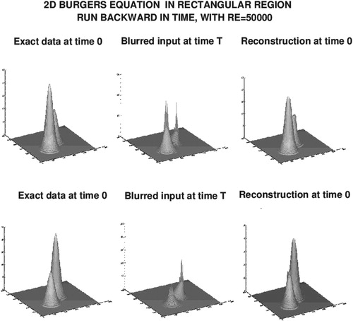
Next, we consider the backward problem. Here, we use the previously computed values at time $T_{max}$ as input data, and apply the stabilized explicit scheme in Equation (38(38) $\begin{array}{rl}{\tilde{u}}^{n+1}& =S{\tilde{u}}^n+\mathrm{\Delta }tS{L}_1{\tilde{u}}^n,\\ {\tilde{v}}^{n+1}& =S{\tilde{v}}^n+\mathrm{\Delta }tS{L}_2{\tilde{v}}^n,n=0,1,\dots ,N.\end{array}$(38) ). With a uniform grid on the unit square Ω, FFT algorithms are the natural tool to use in synthesizing the smoothing operator S which is based on $(-\mathrm{\Delta }{)}^p$. After a few interactive parameter trials, values of $\omega =1.0\times {10}^{-9}$, together with p=3.0, were arrived at. Because of the S-induced unconditional stability, it was possible to use a value of $|\mathrm{\Delta }t|$ five times larger in the backward computation, namely, $\mathrm{\Delta }t=-5.0\times {10}^{-8},(N+1)=50,000$. The resulting recovered initial values are plotted in the right column of Figure 1. The maximum values in the recovered data are 46.7, as compared to the true values of 50.0.

5.2. Image experiment at $\mathrm{RE}=3400$

Our next experiment, illustrated in Figures 2 and 3, involves $256\times 256$ pixel grey scale images, defined on the unit square Ω. As is well known, many natural images are generated by highly non-smooth intensity data. Use of such data in ill-posed time-reversed evolution equations, presents significant challenges to any reconstruction algorithm. At the same time, the use of images is particularly instructive as it enables visualizing the distortion produced by the forward evolution, together with the subsequent attempt at undoing that distortion by marching backward in time.

Figure 2. Using precomputed input data at time $T=2.5\times {10}^{-4}$, shown in middle column, nonlinear explicit scheme in Equation (8(8) $\begin{array}{rl}{\tilde{u}}^{n+1}& =S{\tilde{u}}^n+\mathrm{\Delta }tS{L}_1{\tilde{u}}^n,\\ {\tilde{v}}^{n+1}& =S{\tilde{v}}^n+\mathrm{\Delta }tS{L}_2{\tilde{v}}^n,n=0,1,\dots ,N.\end{array}$(8) ), run backward in time, seeks to recover the true images shown in leftmost column. Actually recovered mages are shown in rightmost column. Notice severe wavy distortion of sea wall in blurred Sydney Opera House image, shown at bottom in middle column, and its successful reconstruction in bottom rightmost image.

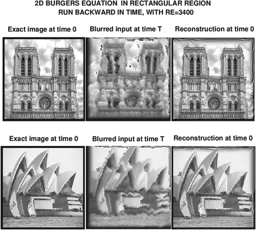
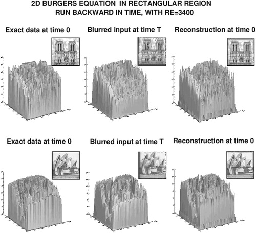
Figure 3. Backward recovery of the underlying intensity data that generate the images in the reconstruction experiment shown in Figure 2.

Here, the 2D Burgers' system in Equation (35(35) $\begin{array}{rl}{u}_t& =L_{1}u\equiv \nu \mathrm{\Delta }u-u{u}_x-v{u}_y,0<t\le T_{max},\\ v_t& =L_{2}v\equiv \nu \mathrm{\Delta }v-u{v}_x-v{v}_y,0<t\le T_{max},\end{array}$(35) ) is used, with $T_{max}=2.5\times {10}^{-4}$, the kinematic viscosity $\nu =0.075$, and homogeneous boundary conditions on $\mathrm{\partial \Omega }$. The initial values are the intensity data, shown in the leftmost column of Figure 3, that define the images shown in the leftmost column of Figure 2. These intensities range from 0 to 255. Accordingly, with $\sqrt{A}=1.0,\nu =0.075,U_{max}=255.0,$ we have $\mathrm{RE}=3400$ in this experiment.

With $|\mathrm{\Delta }t|=8.33\times {10}^{-10},(N+1)=300,000,T_{max}=(N+1)|\mathrm{\Delta }t|$, and S chosen as the identity operator in Equation (38(38) $\begin{array}{rl}{\tilde{u}}^{n+1}& =S{\tilde{u}}^n+\mathrm{\Delta }tS{L}_1{\tilde{u}}^n,\\ {\tilde{v}}^{n+1}& =S{\tilde{v}}^n+\mathrm{\Delta }tS{L}_2{\tilde{v}}^n,n=0,1,\dots ,N.\end{array}$(38) ), stable computation of the forward problem on a uniform grid with $\mathrm{\Delta }x=\mathrm{\Delta }y=1.0/256$, produced the blurred images shown in the middle column of Figure 2.

In the absence of the leftmost and rightmost columns in Figure 2, the images in the middle column of that figure, when magnified, are almost unrecognizable, due to the severe blurring caused by the forward evolution. In particular, the sea wall surrounding the Sydney Opera House develops a striking wavy pattern in the bottom middle image, reflecting some form of turbulence associated with Burgers' equation. Such severe distortion is noteworthy, as each of $T_{max}$ and RE, are one order of magnitude smaller than was the case in the previous Gaussian data experiment.

Next, using the intensity data in the middle column of Figure 3 as input at $T_{max}=2.5\times {10}^{-4}$, we apply the stabilized explicit scheme in Equation (38(38) $\begin{array}{rl}{\tilde{u}}^{n+1}& =S{\tilde{u}}^n+\mathrm{\Delta }tS{L}_1{\tilde{u}}^n,\\ {\tilde{v}}^{n+1}& =S{\tilde{v}}^n+\mathrm{\Delta }tS{L}_2{\tilde{v}}^n,n=0,1,\dots ,N.\end{array}$(38) ) to march backward in time. With $\omega =3.0\times {10}^{-9},p=3.25$, in the FFT-synthesized smoothing operator S, and a value of $|\mathrm{\Delta }t|$ three times larger than in the forward problem, we obtain the images shown in the rightmost column of Figure 2. These are the images defined by the recovered intensity data shown in the rightmost column of Figure 3. Evidently, credible reconstruction has been achieved, although the recovered images and data differ qualitatively and quantitatively from the exact values. However, such discrepancies are to be expected in ill-posed continuation from noisy data.

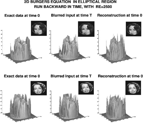
5.3. Image experiment in non-rectangular region at $\mathrm{RE}=2500$

In rectangular regions Ψ, the Fast Fourier Transform is an efficient tool for synthesizing $(-\nu \mathrm{\Delta }{)}^p$ for positive non-integer p. This was used to advantage in the previous two experiments. However, as was shown in [25, 26], and will be shown again below, FFT Laplacian smoothing may be feasible for the 2D Burgers' equation in non-rectangular regions Ω, with zero Dirichlet data on an assumed smooth boundary $\mathrm{\partial \Omega }$. Enclosing Ω in a rectangle Ψ, a uniform grid is imposed on Ψ, fine enough to sufficiently well approximate $\mathrm{\partial \Omega }.$ The discrete boundary $\mathrm{\partial }{\mathrm{\Omega }}_d,$ consisting of the grid points closest to $\mathrm{\partial \Omega },$ is then used in place of $\mathrm{\partial \Omega }$. We use centred finite differencing for the spatial derivatives in $L_1,L_2,$ in Equation (35(35) $\begin{array}{rl}{u}_t& =L_{1}u\equiv \nu \mathrm{\Delta }u-u{u}_x-v{u}_y,0<t\le T_{max},\\ v_t& =L_{2}v\equiv \nu \mathrm{\Delta }v-u{v}_x-v{v}_y,0<t\le T_{max},\end{array}$(35) ). At each time step n in Equation (38(38) $\begin{array}{rl}{\tilde{u}}^{n+1}& =S{\tilde{u}}^n+\mathrm{\Delta }tS{L}_1{\tilde{u}}^n,\\ {\tilde{v}}^{n+1}& =S{\tilde{v}}^n+\mathrm{\Delta }tS{L}_2{\tilde{v}}^n,n=0,1,\dots ,N.\end{array}$(38) ), after applying the operators $(I+\mathrm{\Delta }t{L}_1),(I+\mathrm{\Delta }t{L}_2),$ to ${\tilde{u}}^n,{\tilde{v}}^n,$ respectively, on $\mathrm{\Omega }\subset \mathrm{\Psi }$, these discrete functions are then extended to all of Ψ by defining them to be zero on the grid points in $\mathrm{\Psi }-\mathrm{\Omega }$. FFT algorithms are then applied on Ψ to synthesize S in Equation (38(38) $\begin{array}{rl}{\tilde{u}}^{n+1}& =S{\tilde{u}}^n+\mathrm{\Delta }tS{L}_1{\tilde{u}}^n,\\ {\tilde{v}}^{n+1}& =S{\tilde{v}}^n+\mathrm{\Delta }tS{L}_2{\tilde{v}}^n,n=0,1,\dots ,N.\end{array}$(38) ), and produce ${\tilde{u}}^{n+1},{\tilde{v}}^{n+1}.$ Retaining only the values of these discrete functions on Ω, the process is repeated at the next time step.

The last experiment, illustrated in Figures 4 and 5, involves recognizable face images defined on an elliptical domain Ω, with area A=0.544, enclosed in the unit square Ψ. As before, the kinematic viscosity $\nu =0.075,$ and $U_{max}=\mathrm{255.0.}$ With $\sqrt{A}=0.738$, we now have $\mathrm{RE}=2500$. A $256\times 256$ grid was placed on Ψ. As in the previous experiment, with S the identity operator, $|\mathrm{\Delta }t|=4.17\times {10}^{-10},(N+1)=600,000,T_{max}=(N+1)|\mathrm{\Delta }t|=2.5\times {10}^{-4}$, stable forward computation in Equation (38(38) $\begin{array}{rl}{\tilde{u}}^{n+1}& =S{\tilde{u}}^n+\mathrm{\Delta }tS{L}_1{\tilde{u}}^n,\\ {\tilde{v}}^{n+1}& =S{\tilde{v}}^n+\mathrm{\Delta }tS{L}_2{\tilde{v}}^n,n=0,1,\dots ,N.\end{array}$(38) ), using the intensity data shown in first column of Figure 5, produced the blurred images in the middle column of Figure 4, and the intensity data in the middle column of Figure 5. Although not as severe as in Figure 2, quite noticeable blurring is evident in Figure 4.

Figure 4. Using precomputed input data at time $T=2.5\times {10}^{-4}$, shown in middle column, nonlinear explicit scheme in Equation (8(8) $\begin{array}{rl}{\tilde{u}}^{n+1}& =S{\tilde{u}}^n+\mathrm{\Delta }tS{L}_1{\tilde{u}}^n,\\ {\tilde{v}}^{n+1}& =S{\tilde{v}}^n+\mathrm{\Delta }tS{L}_2{\tilde{v}}^n,n=0,1,\dots ,N.\end{array}$(8) ), run backward in time, seeks to recover the true images shown in leftmost column. Actually recovered images are shown in rightmost column.

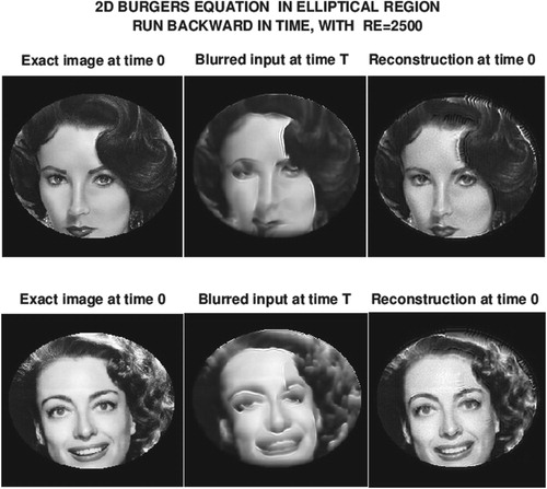
Figure 5. Backward recovery of the underlying intensity data that generate the images in the reconstruction experiment shown in Figure 4.

Next, using the intensity data in the middle column of Figure 5 as input at $T_{max}=2.5\times {10}^{-4}$, we apply the stabilized explicit scheme in Equation (38(38) $\begin{array}{rl}{\tilde{u}}^{n+1}& =S{\tilde{u}}^n+\mathrm{\Delta }tS{L}_1{\tilde{u}}^n,\\ {\tilde{v}}^{n+1}& =S{\tilde{v}}^n+\mathrm{\Delta }tS{L}_2{\tilde{v}}^n,n=0,1,\dots ,N.\end{array}$(38) ) to march backward in time, using the FFT strategy outlined in the first paragraph. With $\omega =4.0\times {10}^{-10},p=3.5,$ in the smoothing operator S, and a value of $|\mathrm{\Delta }t|$ 10 times larger than in the forward problem, we obtain the images shown in the rightmost column of Figure 4. These are the images defined by the recovered intensity data shown in the rightmost column of Figure 5. Again, quite good reconstructions are obtained, despite inevitable discrepancies between the exact and recovered data and images in Figures 4 and 5.

6. Concluding remarks

To the author's knowledge, successful backward in time computations in the 2D Burgers' equation, have not previously appeared in the literature. The results obtained here offer a glimpse of what might be feasible, although the stabilized explicit scheme in Equation (8(8) $\begin{array}{rl}{\tilde{u}}^{n+1}& =S{\tilde{u}}^n+\mathrm{\Delta }tS{L}_1{\tilde{u}}^n,\\ {\tilde{v}}^{n+1}& =S{\tilde{v}}^n+\mathrm{\Delta }tS{L}_2{\tilde{v}}^n,n=0,1,\dots ,N.\end{array}$(8) ) will generally be useful only in a limited class of problems. The successful first experiment in Section 5, at $\mathrm{RE}=50,000$, is noteworthy even though relatively simple data were involved. The second experiment, at a much smaller Reynolds number, was instructive in highlighting the severe distortions that can occur with highly complex non-smooth data, and the remarkable backward recovery that yet remains possible. The last experiment is important in illustrating the possible use of FFT-synthesized smoothing operators in non-rectangular regions.

Theoretical error estimates for backward reconstruction from noisy data, such as are given in [15–19], necessarily reflect worse case error accumulation scenarios, and may be too pessimistic in individual situations. As in [23–26], the use of 8 bit grey scale images provide challenging test examples, as well as an instructive way of exploring the feasibility of backward recovery with various types of complicated non-smooth data.

Disclosure statement

No potential conflict of interest was reported by the author.

References

- Cole JD. On a quasi-linear parabolic equation occurring in aerodynamics. Quart Appl Math. 1951;3:225–236. doi: 10.1090/qam/42889
- Abazari R, Borhanifar A. Numerical study of the solution of the Burgers and coupled Burgers equations by a differential transformation method. Comput Math Appl. 2010;59:2711–2722. doi: 10.1016/j.camwa.2010.01.039
- Zhu H, Shu H, Ding M. Numerical solutions of two-dimensional Burgers' equations by discrete Adomian decomposition method. Comput Math Appl. 2010;60:840–848. doi: 10.1016/j.camwa.2010.05.031
- Srivastava VK, Tamsir M, Bhardwaj U, et al. Crank-Nicolson scheme for numerical solutions of two-dimensional coupled Burgers' equations. Int J Sci Eng Res. 2011;2:1–7.
- Khan M. A novel technique for two dimensional Burgers equation. Alexandria Eng J. 2014;53:485–490. doi: 10.1016/j.aej.2014.01.004
- Wang Y, Navon IM, Wang X, et al. 2D Burgers equation with large Reynolds number using POD/DEIM and calibration. Int J Numer Meth Fluids. 2016;82:909–931. doi: 10.1002/fld.4249
- Zhanlav T, Chuluunbaatar O, Ulziibayar V. Higher-order numerical solution of two-dimensional coupled Burgers' equations. Am J Comput Math. 2016;6:120–129. doi: 10.4236/ajcm.2016.62013
- Ou K, Jameson A. Unsteady adjoint method for the optimal control of advection and Burgers' equation using high order spectral difference method. 49th AIAA Aerospace Science Meeting, 2011 January 4–7; Orlando, FL.
- Allahverdi N, Pozo A, Zuazua E. Numerical aspects of large-time optimal control of Burgers' equation. ESAIM Math Model Numer Anal. 2016;50:1371–1401. doi: 10.1051/m2an/2015076
- Gosse L, Zuazua E. Filtered gradient algorithms for inverse design problems of one-dimensional Burgers' equation. In: Gosse L, Natalini R, editors. Innovative algorithms and analysis. SINDAM Series. Springer; 2017. p. 197–227. doi: 10.1007/978-3-319-49262-9_7
- Lundvall J, Kozlov V, Weinerfelt P. Iterative methods for data assimilation for Burgers' equation. J Inv Ill-Posed Problems. 2006;14:505–535. doi: 10.1515/156939406778247589
- Auroux D, Blum J. A nudging-based data assimilation method for oceanographic problems: the back and forth nudging (BFN) algorithm. Proc Geophys. 2008;15:305–319. doi: 10.5194/npg-15-305-2008
- Auroux D, Nodet M. The back and forth nudging algorithm for data assimilation problems: theoretical results on transport equations. ESAIM:COCV. 2012;18:318–342. doi: 10.1051/cocv/2011004
- Auroux D, Bansart P, Blum J. An evolution of the back and forth nudging for geophysical data assimilation: application to Burgers' equation and comparison. Inverse Probl Sci Eng. 2013;21:399–419. doi: 10.1080/17415977.2012.712528
- Carasso A. Computing small solutions of Burgers' equation backwards in time. J Math Anal App. 1977;59:169–209. doi: 10.1016/0022-247X(77)90100-7
- Hào DN, Nguyen VD, Nguyen VT. Stability estimates for Burgers-type equations backward in time. J Inverse Ill Posed Probl. 2015;23:41–49. doi: 10.1515/jiip-2013-0050
- Knops RJ, Payne LE. On the stability of solutions of the Navier-Stokes equations backward in time. Arch Rat Mech Anal. 1968;29:331–335. doi: 10.1007/BF00283897
- Payne LE, Straughan B. Comparison of viscous flow backward in time with small data. Int J Nonlinear Mech. 1989;24:209-214. doi: 10.1016/0020-7462(89)90039-5
- Knops RJ. Logarithmic convexity and other techniques applied to problems in continuum mechanics. In: Knops RJ, editor. Symposium on non-well-posed problems and logarithmic convexity. Vol. 316, Lecture notes in mathematics. New York (NY): Springer-Verlag; 1973. p. 31–54.
- Lattès R, Lions JL. Méthode de Quasi-Réversibilité et Applications [The method of quasi-reversibility and applications]. Paris: Dunod; 1967.
- Ames KA, Straughan B. Non-standard and improperly posed problems. New York (NY): Academic Press; 1997.
- Carasso AS. Reconstructing the past from imprecise knowledge of the present: effective non-uniqueness in solving parabolic equations backward in time. Math Methods Appl Sci. 2012;36:249–261. doi: 10.1002/mma.2582
- Carasso AS. Stable explicit time-marching in well-posed or ill-posed nonlinear parabolic equations. Inverse Probl Sci Eng. 2016;24:1364–1384. doi: 10.1080/17415977.2015.1110150
- Carasso AS. Stable explicit marching scheme in ill-posed time-reversed viscous wave equations. Inverse Probl Sci Eng. 2016;24:1454–1474. doi: 10.1080/17415977.2015.1124429
- Carasso AS. Stabilized Richardson leapfrog scheme in explicit stepwise computation of forward or backward nonlinear parabolic equations. Inverse Probl Sci Eng. 2017;25:1–24. doi: 10.1080/17415977.2017.1281270
- Carasso AS. Stabilized backward in time explicit marching schemes in the numerical computation of ill-posed time-reversed hyperbolic/parabolic systems. Inverse Probl Sci Eng. 2018;1:1–32. doi: 10.1080/17415977.2018.1446952