An inverse problem approach to stiffness mapping for early detection of breast cancer: tissue phantom experiments

ABSTRACT

Early detection of breast cancer will continue to be crucial in improving patient survival rates. Our ultimate goal is to develop an electro-mechanical device to automate and refine the manual breast exam process, and use inverse techniques to generate a tissue stiffness map of the breast tissue. We have previously presented computational simulations of the stiffness mapping approach, which employs static indentations of the tissue and measurements of surface displacements. In this paper, we report on experimental validation of the technique with tissue phantom experiments. We tested 12 tissue phantom samples without simulated tumours and 14 tissue phantom samples with simulated tumours. Our stiffness mapping approach correctly identified all 26 samples.

KEYWORDS:

• Breast cancer
• inverse problems
• genetic algorithm
• finite elements

SUBJECT CLASSIFICATION CODE:

• 65M32

1. Introduction

Early detection of breast cancer will continue to be crucial in improving patient survival rates. Manual breast exams (breast palpation) and mammograms are currently the most effective and widely used early detection techniques [1,2]. Unfortunately, manual breast exams are limited in their ability to detect tumours since they only produce local information about the site where the force is applied and do not provide quantitative (recordable) measurements for comparison with future exams. Mammograms, while effective, expose the patient to radiation and hence routine mammograms are limited to those in specific age or risk groups. In addition, mammograms do not quantify tissue stiffness, an identifying characteristic of breast tumours (it is widely agreed that cancerous tissue has a Young's modulus (stiffness) as much as 10 times that of the surrounding breast tissue [3,4]).

Our ultimate goal is to develop a system that automates, quantifies, and enhances the resolution of the manual breast exam. An electro-mechanical device will gently indent the tissue surface in various locations, recording the tissue surface deflections on the entire tissue surface (note that we will record only the final deflections for each indentation site, not their time histories ). This deflection data will be used with inverse techniques involving finite element methods and genetic algorithms to provide detailed three-dimensional (3D) maps of the Young's modulus of the interior of the breast tissue. These 3D maps could then be used to identify any suspicious sites. These maps could also provide quantitative values for comparing baseline data (which could be taken at an early age since there is no radiation or other risk to the patient) with data taken on subsequent visits, providing yet another mechanism for early identification of cancerous sites. If suspicious sites are identified, we envision that clinicians would employ mammography, ultrasound, and other imaging modalities to investigate further.

In practice we anticipate that the procedure would occur as follows:

1. The patient would lie supine on the examining table, and an electro-mechanical device will gently indent the breast surface in various locations

2. For each indentation site, the displacements over the breast tissue surface would be recorded as the ‘measured result’.

3. A genetic algorithm would be used to infer the tissue stiffness map in a finite element model of the breast.

We have previously [5] discussed computational simulations of this process. In this paper, we report on the validation of the approach using tissue phantom experiments. Section 2 discusses related work in this field, Section 3 reviews our computational approaches, Section 4 describes the experimental procedures for the tissue phantom experiments, Section 5 presents the results of our testing, and Section 6 summarizes our work and suggests avenues for further development.

2. Background literature

Existing studies on identifying stiffer cancerous tissues in otherwise healthy breast tissue fall into two broad categories– methods that require the displacement field (or strain field) within the breast tissue and methods that measure pressures/forces or displacements on the breast surface.

2.1. Methods that require the displacement field within the breast tissue

Greenleaf, Fatemi, and Insana [4], Parker [6], and Parker, Doyley, and Rubens [7] provide reviews of the first class of techniques, which are referred to by a variety of names, including ‘elastography’, ‘elasticity imaging’, ‘elastic modulus imaging’, ‘ultrafast imaging’, and ‘vibroacoustography’. Each of these methods uses formal inverse techniques to infer the shear modulus or Young's modulus distribution in the breast tissue from measurements of the displacement or strain throughout the interior of the breast. The methods differ in the loading used to cause the displacements (external static loads, external time-dependent loads, or internal time-dependent loads), and the methods used to measure the displacements (typically ultrasound-based or magnetic resonance-based techniques).

Recent work on this approach includes studies by Barbone, Oberai, and their colleagues [8–24]. Their methods employ quasi-static displacement measurements with nonlinear anisotropic material models, and they report experimental results for tissue phantoms and in preliminary in-vivo studies. In Goenezen et al. [13] they seek to determine whether identified tumours in particular regions of interest are benign or malignant. Park and Maniatty [25,26] start from time-dependent displacement data to solve the dynamic equilibrium equations for the shear modulus field. McLaughlin and her colleagues [27–31] also study solutions to the dynamic elastography problem and present results from in-vivo testing in the liver and the spleen. Greenleaf, Fatemi, and their co-workers [32–38] employ vibroacoustography (a dynamic response excited by ultrasound radiation forces). They have reported promising results in ex-vivo studies of prostate tissue and are working to develop clinically applicable scanners. Perrinez et al. [39] examine the ability of time-harmonic magnetic resonance elastography to reconstruct material properties for poroelastic (tofu) phantoms and find that linear elastic models are insufficient. Continuing this work, Perreard et al. [40] examine the effects of mismatches between the assumed material model and the actual material response of their phantoms. They found that treating poroelastic or anisotropic materials as linear isotropic elastic materials caused substantial errors. Eskandari et al. [41] and Guo et al. [42] have investigated numerical techniques for elastography which improve the speed of reconstructions. This first category of techniques – methods requiring internal fields – has a rich history of contributions by many researchers [43–61].

The methods in this first group all employ ultrasound, magnetic resonance, or computed tomography techniques to measure the displacements within the breast tissue, and they require relatively sophisticated equipment (and in some cases exposure to radiation). While they show promise for localizing already-identified tumours more accurately and non-invasively characterizing tissue pathology, they are unlikely to be used for routine screening of all patients in the near future.

2.2. Methods that measure pressures/forces or displacements on the breast surface

Studies related to ‘tactile imaging’, ‘mechanical imaging’, or ‘palpation imaging’ take a fundamentally different approach. Here a transducer (similar to an ultrasound wand) is manually scanned over the breast surface. The transducer measures reaction pressures, and the patterns overlap to form a full map of the reaction pressures. In her thesis, Wellman [62] gave some preliminary results on matching the surface pressure distributions to typical tumour locations, and also reported on clinical use of the scanning device. Wellman et al. [63] report on clinical scans of women preparing to undergo surgery, and hence with known breast lumps. The estimates of lump size compared well with post-surgical lump size measurements and were more accurate than values from manual palpation or ultrasound. However, these size estimates were based on heuristics rather than a formal inverse procedure. Kaufman et al. [64] explore the use of palpation imaging as a method for documenting the breast examination. Weiss et al. [65] and Niemczyk et al. [66] report on pilot studies of a mechanical imaging device for use in detecting prostate cancer, which, like breast cancer, is often identified through manual palpation. In related work, Sallaway et al. [67] studied the force-deflection patterns associated with breast palpation in a model system consisting of gelatin phantoms containing spherical steel inclusions.

Sarvazyan, Egorov, and their colleagues have continued to develop this type of approach in their ‘Mechanical Imaging’ or ‘Tactile Imaging’ work [68–75] They have applied the technique to prostate, breast, female pelvic floor, and muscle tissues. For the breast examination application, surface stress patterns are measured by a wand which is scanned over the surface of the breast. From this data, a semi-empirical approach is used to create a 3D image of the breast [74]. This device is now FDA approved as a Class II medical device and marketed for clinical use under the trade name ‘SureTouch’. The main audience for the device is women who refuse regular mamographic screening, women under 40 who seek screening, and women who have contraindications to radiation and severe breast compression [76]. As reported in 2014 [77], for symptomatic patients the sensitivity and specificity of the SureTouch device was comparable to other standard imaging modalities such as manual palpation, mammograms, and ultrasound.

Shih, Shih, and their co-workers have developed a device they term a ‘piezo-electric finger’ or PEF [78–83]. This is a flexible cantilever with attached force/displacement sensors which is scanned over the tissue surface. They map their results to a 1D equation to infer the tissue stiffness beneath the surface. Their recent work [78,79] has advanced to in-vivo testing on patients with already-identified breast abnormalities. In [78] they tested 39 patients with abnormalities and 1 patient without abnormalities and PEF gave a correct overall identification for each patient. Of the 46 lesions, PEF identified 55 lesions. Two of the lesions were true positives that had been missed by imaging and palpation, 9 of the lesions were false positives, and the remaining 46 lesions were correctly identified by PEF and imaging/palpation. In their most recent work [79] they again conduct it in-vivo testing of 40 patients (1 normal and 39 abnormal), this time to determine the effects of various examination parameters. They find that the indentation depth and the hold time for a given testing site do not substantially affect the quality of the results. In the 40 patients, PEF detected 46/48 lesions. These results were independent of breast density. Since they have not reached the stage of testing where a larger number of normal patients could be included, it is not yet possible to know the rate of false positives for general screening.

Yen et al. [84] attach force and displacement sensors to an ultrasound wand and also attempt to characterize lumps previously identified through ultrasound techniques.

As with our proposed technique, these methods use surface measurements. However, the force/displacement measurements are only taken at the site where the forces are applied, and geometry and displacement data away from the forced locations are not recorded. Heuristic or approximate relationships are used to characterize the previously located tumours.

Chase and VanHouten have worked on Digital Image-based Elasto-Tomography, or DIET [85–92]. They apply an external sinusoidal excitation to the breast surface, and measure the steady-state motion of the tissue surface with digital cameras. Computational problems associated with calculating surface displacements from multiple camera images have received much of their attention [85,91,92]. In Peters et al.[89,90,93], they present experimental and computational results from silicone phantoms. In [89] one of the phantoms is stacked – a soft cylinder on top of a stiff cylinder – while the other is concentric – a soft cylinder surrounding a stiff cylinder. At that stage, even for large inclusions, they were encountering difficulty in reconstructing the stiffnesses and sizes in the concentric case. More recently [94], they have presented a method for identifying the presence of tumours by identifying local variations in the first two resonant modes of the breast. Tests on tumour-containing phantoms indicated that the presence of a tumour could be identified reliably for samples with 10 mm or larger tumours. Tumours were always placed at the 6 o'clock location for testing, and the specific tumour location is not identified with this approach. The DIET method involves a steady dynamic excitation in contrast to the static deformations that we propose, thus introducing tissue density into the calculations in addition to stiffness.

In summarizing this section, we would like to emphasize that our proposed approach is distinct from all of these methods. We seek to develop inverse techniques which infer (or map) the stiffness throughout the breast tissue based only on a knowledge of quasi-static surface displacements, systematizing techniques used in breast palpation.

2.3. Material models and properties for breast tissues

In order to test and refine approaches to estimating the stiffness of breast tissues, we need reliable information on material models and properties of breast tissues.

Although the response of breast tissue for small strains can be modelled as incompressible linear elastic, for larger strains a nonlinear viscoelastic material model is generally considered to be more appropriate. Greenleaf, Fatemi, and Insana [4] discuss material properties for biological tissues. Krousop et al. [95] measured the moduli for breast tissue assuming a linear elastic model. They found that the modulus of some tissues varied with strain, but only for strains of the order of 20–30%. For strains up to 10%, the modulus was nearly constant. Samani et al. [3,96] provide more recent extensive tissue data which included 169 tissue samples. Using a linear elastic model for the tissues, fat had a Young's modulus of 3.25±0.91 kPa, which was similar to healthy fibroglandular tissue at 3.24±0.61 kPa. In contrast, intermediate-grade IDC (Invasive Ductal Carcinoma) had a stiffness of 19.99±4.2 kPa and high-grade IDC was 42.52±12.47 kPa. They concluded that a linear elastic model was adequate for cancerous tissues. They examined this issue again [97–99], utilizing experiments to fit healthy and cancerous tissues to hyperelastic material models of various types. The nonlinear material parameters for healthy and pathological tissues showed distinct differences. In addition to their work on linear elastography methods, Barbone and Oberai and their colleagues have studied nonlinear material models for elastography [14,16,18]. They conclude that the nonlinear term in the material model is a better discriminator of tumour type (benign, cancerous). However, for our purposes, it is more important that they conclude that small strain results are essentially independent of the nonlinear term and that the tumour itself rarely sees large strains, since it is embedded in substantially less stiff tissues.

Based on this literature, we designed our experimental validation to minimize nonlinear effects and to use a healthy tissue stiffness of approximately 2.3 kPa and a cancerous tissue stiffness of approximately 18.5 kPa. To minimize deviations from linear elasticity the experiments involved only small quasi-static indentations. The tissue phantoms were created from gelatin compositions that had been separately verified to have the desired healthy and cancerous stiffness. This is discussed in more detail in Section 4. Our computational algorithms use an incompressible linear elastic material model with those same healthy and cancerous stiffness values.

2.4. Breast volume

Few studies report data on breast volumes. The International Commission on Radiological Protection [100] established a reference value of 500 g for total breast mass and a specific gravity of 1.05, or 238 cc volume for a single breast. Westreich [101] reports values for 50 women, all with ‘aesthetically perfect’ breasts. Smith et al. [102] obtained data from 55 more typical female volunteers and reports a median volume of approximately 220 cc. Loughry et al. [103,104] used biostereometric analysis to evaluate 598 randomly chosen women who received mammograms at Akron City Hospital. This is a large sample and the volume information was acquired in a systematic fashion. They report an average breast volume of 203 cc with a median somewhat lower at approximately 170 cc. Our testing used a 180 g domain, which appears to be a reasonable starting point given the limited data available (the gelatin mixtures we use have a density very close to 1 g/cc). Note that this starting point would represent an average patient, rather than an overweight or obese patient, and additional sizes of tissue phantoms would need to be considered in future studies.

3. Numerical methods

The numerical methods we use in this work have been described in a related form in a previous paper [5], and we review them here for clarity. Our stiffness mapping approach assumes that we have indented the tissue surface at particular locations and have measured the resulting normal surface displacements across the majority of the tissue surface (as described in Section 4). We create a finite element model (FEM) of the breast tissue. We then use a genetic algorithm to find the element stiffnesses in the model so that the response of the FEM best matches the measured normal displacements.

With the experimentally measured surface displacements and tissue geometry as input, the genetic algorithm operates in the following way:

• Create an initial population of individuals. Each individual is a FEM of the breast with an assumed stiffness map.

• For each generation

  	-	Apply indentation test patterns to FEM individuals and record FEM surface displacements
  	-	Assign a ‘fitness’ to each individual – how close is the FEM response to the measured response?
  	-	Select top individuals as ‘parents’, discard others
  	-	Mate parents to create new individuals (‘children’).
  	-	Introduce mutations into some children

• Repeat generations until convergence: report and plot the most fit FEM individual as the final ‘stiffness map’

For the purposes of this testing, we ran the genetic algorithm with 320 individuals per generation and 50 generations. Although ultimately we would seek a convergence criteria to set the number of generations, for our purposes the algorithm was seen to have converged well within the 50 generations and that was held fixed for our testing.

Notice that the ‘best match’ between the FEM individual's response and the measurement is determined by the selected ‘fitness’, and that the genetic algorithm is merely a systematic approach to finding this optimal match.¹ We refer to the combination of the finite element modelling and optimal matching with the genetic algorithm as ‘stiffness mapping’ since it takes the measured data as an input and produces a 3D stiffness map as an output. More details on the process are given in the remainder of this section.

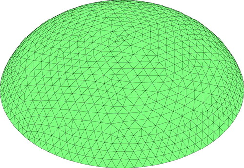
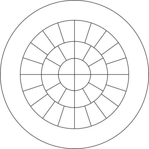
Individuals are created as finite element models of the tissue volume, as shown in Figure 1. Elements in the mesh are chosen to have either ‘healthy’ (Young's modulus $E_h$=2.3 kPa) or ‘cancerous’ (Young's modulus $E_c$=18.5 kPa) tissue, and this choice defines the individual. The finite elements themselves are nearly incompressible (ν=0.49) displacement/pressure elements [105]. The finite element solver is a custom, fully validated code which is fully integrated with the genetic algorithm for efficiency [5].

Figure 1. Typical finite element mesh generated for an individual.

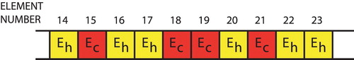
The information about the individuals is coded into a ‘chromosome’ (see Figure 2) which lists the material properties for each of the elements. Once the finite element meshes and material properties for each individual are defined, it is straightforward to apply the indentation patterns to the model and determine the surface normal displacements for each FEM individual.

Figure 2. Chromosome used to encode material property information for each individual ($E_h$ is healthy modulus, $E_c$ is cancerous modulus).

We assign the fitness of each individual based on its ‘Cost’: (1) $\text{Cost}=\frac{\delta }{{\delta }_{tf}}+w\frac{R_{tumour}}{R_{entire}}.$(1) Here δ is the sum of absolute errors between the individual's normal displacements and the measured normal displacements, summed over all indentation sites; ${\delta }_{tf}$ is the value of δ for a tumour-free individual; $R_{tumour}$ is an effective tumour radius; and $R_{entire}$ is the effective radius of the entire tissue (these terms are described more precisely in Appendix. Note that the tumour and entire tissue are not assumed to be spherical, $R_{tumour}$ and $R_{entire}$ are merely size estimates). In this equation, the first term represents the fit between the measured data and the response of the FEM individual. As for other inverse problems, simply finding the best fit to the data will generally lead to unstable solutions unless some form of regularization is employed. The second term in the Cost equation is the regularizer which favours compact tumours over larger or more widely dispersed tumours and w is the adjustable weighting parameter.

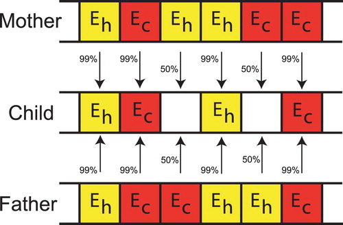
The lowest cost individuals are the most fit, and we choose 16 as parents for the next generation. Parents are mated in pairs to produce children as shown in Figure 3. If both parents have the same gene the child has a 99% chance of having that gene. If the parents have different genes then the child has an equal chance of a healthy or cancerous gene. Once the children are created mutations are introduced in the children. A random number of children, up to 50%, are selected for mutation. On those selected a random number of genes, up to 50%, are mutated. A mutation consists of changing the gene from healthy to cancerous or cancerous to healthy. Parents are retained for the next generation.

Figure 3. Mating parents to produce children.

We constrain the genetic algorithm to modify the materials only in 144 centrally located ‘clumps’ of elements. This allows us to reduce the search space without coarsening the underlying finite element mesh. Figure 4 showing the clumps in a cross-section through the mesh. The clumps of elements are assigned by slicing the mesh radially, circumferentially, and vertically to produce clumps that each have a volume of approximately one cubic centimetre. Figure 5 shows a schematic top view of the slices. (The process for creating clumps is described in more detail in our previous paper [5].) We exclude the edges of the domain from the clumping process and from the search space of the genetic algorithm (the edges of the domain would be filled from bottom to top by tumour material if a one cc tumour were placed there).

Figure 4. Cross-section of mesh with element clumps.

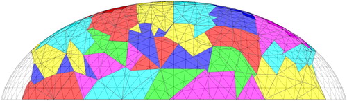
Figure 5. Schematic top view of slices used to create clumps.

The first generation of the genetic algorithm consists (as do all the generations) of 320 individuals. We seed the first generation with a tumour-free individual, as well as 144 individuals each with a single cancerous clump of elements. The remaining 175 individuals in the first generation are created by randomly choosing some clumps to be cancerous and some clumps to be healthy tissue.

We note that the genetic algorithm we employ is more effective than an exhaustive search. We have 144 clumps of element each of which can have 2 possible stiffnesses. For an exhaustive search, we would need to examine 2¹⁴⁴=2.2×10⁴³ cases. The genetic algorithm examines 50 generations of 320 individuals, or 1.6×10⁴ cases.

Nevertheless, our algorithm is computationally intensive. We have parallelized the code using MPI and run on the Texas Advanced Computing Center's Stampede2 computers. The wall-clock time for four nodes is 3.5 h.

4. Experimental methods

The experiment consists of three stages:

1. Phantom creation and characterization: Create gelatin tissue phantoms with and without tumours

2. Indentation experiments: Measure surface displacements on tissue phantoms undergoing indentation

3. Data postprocessing: Use genetic algorithm to identify tumour locations

4.1. Phantom creation and characterization

Tissue phantoms were created using 250 Bloom Type B gelatin powder (Custom Collagen, Addison, IL). Gelatin powder was first mixed at the approximate concentration with deionized water and then heated in a 70${}^{\circ }$ C water bath with gentle stirring. After one hour, the gelatin would be fully dissolved and 0.6 g Germall² was added. Next, makeup deionized water was added to achieve the precise concentration desired.

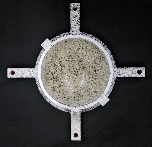
Tumour-free tissue phantoms, such as the one depicted in Figure 6, were prepared by pouring 180 g of a 4% wt solution of gelatin into a roughly hemispherical 120 mm diameter mold³ and sealing the mold to prevent evaporation. The 180 g of solution filled the mold to a depth of approximately 35 mm and the diameter of the free surface in the mold was approximately 107 mm.

Figure 6. Tumour-free tissue phantom. Left: cast in mold, Right: on testing tray.

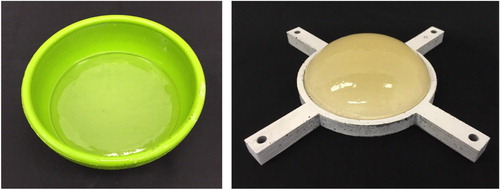
The phantom was allowed to sit for approximately one day (24±2 h), then it was carefully demolded and placed on an appropriately sized testing tray (Figure 6). The phantom ‘slumps’ when placed on the tray and takes on an ellipsoidal shape. Testing trays with diameters of 110, 109, 108, and 107 mm were available. For each sample, the tray which firmly restrained the outer diameter of the phantom, without pinching, was selected. Controlling the gelatin concentration and cure time controls the stiffness of the phantom [106]. Hence, consistently sized tissue phantoms were created by controlling gelatin concentration, cure time, and phantom volume. The actual geometry for any given phantom is identified during data postprocessing, as described in Section 4.3.

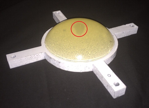
For phantoms containing tumours, a 13% wt solution of gelatin would be prepared the prior day and allowed to set for one day in a petri dish, before being cut into roughly cubical 2 g ‘ tumour' samples⁴. A phantom of 4% wt gelatin would then be prepared as described above, poured into the hemispherical mold, and allowed to cool for 1–2 h (it would not have gelled). The 2 g tumour would then be suspended by a paperclip at the desired location in the 4% wt solution in the ellipsoidal mold, and the mold would be resealed. The 4% wt gelatin containing the tumour would be allowed to set for approximately a day, after which the paperclip would be slowly withdrawn, leaving the tumour in place. Phantoms were then demolded and placed on a testing tray. Figure 7 shows a tissue phantom with a tumour. The volume of the tumours was approximately 2 cm³, corresponding to a cube with 13 mm edges.

Figure 7. Tissue phantom with tumour, on testing tray (circle identifies the tumour).

Gelatin is known to behave viscoelastically, and our previous work describes in more detail the testing and constitutive modelling approaches used with the gelatin used to create these phantoms [106]. Phantom characterization revealed that the gelatin experienced a 10% force relaxation for early times but was largely stable after 15 s. Gelatin stiffness was measured by parallel plate compression (0.5$\mathrm{\%}/s$ strain rate) of gelatin cylinders cast in molds made from sections of PVC piping. The Young's modulus was obtained by linear regression of the stress-strain data between 0.5% and 3.0% strain. The more compliant background gelatin (4% wt) had a measured stiffness of 2.32±0.16 kPa, while the stiffer tumour gelatin (13% wt) was measured at 24.9±2.6 kPa when tested before placement in the background gelatin. However, analysis of gelatin tumours that were excised from background gelatin after curing showed that the gelatin tumour would absorb water osmotically from the background gelatin, leading to a decrease in the tumour's effective concentration. In some tests, the tumour gelatin absorbed enough water that its concentration dropped nearly 1% wt. Because it was experimentally difficult to obtain clean enough margins to directly measure the Young's modulus values for excised gelatin tumours, for simulation purposes the assumed Young's modulus of the (initially 13% wt) tumours inside the phantoms was taken to be equal to that of another set of 12% wt gelatin samples that was prepared – this value was 18.5±3.2 kPa.

4.2. Indentation experiments

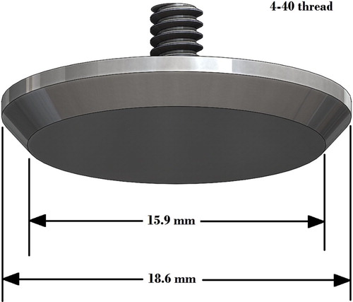
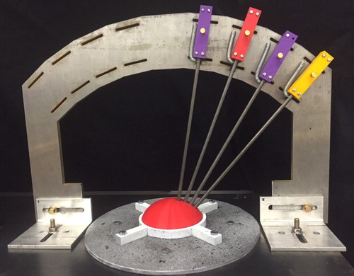
We developed a mechanical ‘Arc’ system (as shown in Figure 8) to apply consistent indentations at known locations normal to the surface of the tissue phantoms. Linear slides hold rods connected to speckled locating cylinders and indenter heads, and a steel frame with adjustable slots holds the slides. This allows us to ensure that the indentations occur normal to the tissue surface at consistent locations, and the locating cylinders allow us to precisely identify those locations. A speckled circular disc holds the tissue phantom testing tray. The disc rotates freely about the centre of the Arc, and can be locked in place at 45 degree intervals. The indenter heads are round with nearly flat faces⁵ as shown in Figure 9. The locating cylinders slide freely up the rods so that images can be captured with and without the cylinders.

Figure 8. ‘Arc’ system for applying consistent indentations (tissue phantom in tray sits on speckled rotatable disc. Linear slides guide rods with locating cylinders and indenter heads. A micrometer holds the rod in place. Rubber bands hold the locating cylinders away from the phantom during indentations).

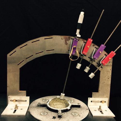
Figure 9. Indenter head geometry.

Before each experiment, the Arc is calibrated by removing the indenter heads and locating cylinders, and inserting the rods into a rapid-prototyped model of the tissue phantom with calibration holes (see Figure 10). The position of the slides is adjusted as necessary within the slots of the steel frame to allow the rods to slide smoothly into the model. Once the Arc is calibrated, the model is removed and the locating cylinders and indenter heads are reattached.

Figure 10. Calibrating the arc (red rapid-prototyped model of tissue phantom contains calibration holes).

After the phantom is placed on the testing tray as shown in Figure 7, speckles are applied⁶ to the phantom for surface displacement tracking (Figure 11).

Figure 11. Tissue phantom with displacement tracking speckles applied.

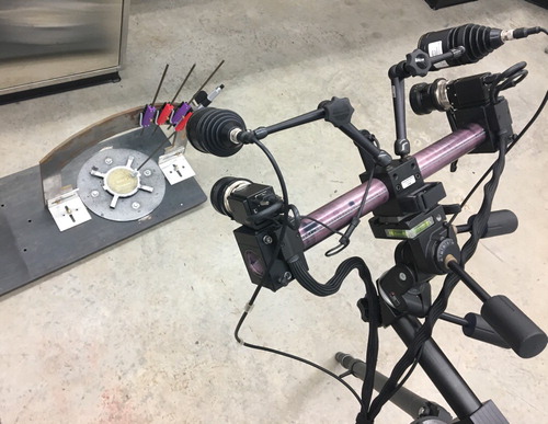
As shown in Figure 12, indentations are applied to the tissue surface and data on phantom surface geometry before and after indentation are captured using an Aramis Optical Deformation Analysis System 5M (GOM). For each indentation location we record full surface data for four conditions: initial contact with a locating cylinder, initial contact, 5 mm indentation, then a second 5 mm indentation (we record two indentation data sets to allow us to average the measurements). The ‘initial contact’ condition is determined with a visual check. Indentation depths are controlled by using a micrometer to enforce displacements at the rod tops (review Figure 8).

Figure 12. Aramis Optical Deformation Analysis System used to acquire surface geometry before and after indentation.

There are a total of 32 indentation locations as shown in Figure 13. Four indenter heads are used to indent the surface for each of the eight possible positions of the circular disc that holds the tissue phantom.

Figure 13. Schematic of top view of tissue phantom illustrating 32 indentation locations.

4.3. Data postprocessing

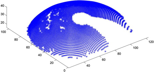
Once the testing is complete, tissue phantom surface position data values are extracted as a point cloud and extraneous points are removed. Figure 14 gives an example of the initial surface points for a particular indentation site (note that the shadow from the indenter – which is not in contact with the surface yet – blocks the camera's view of portions of the surface, resulting in a ‘keyhole’-shaped region of missing data). The set of 32 initial (‘before’) point clouds are fit to an ellipsoid. For the samples in this paper, the ellipsoid fit resulted in a major ellipsoid radius in the range 55–58 mm, a minor ellipsoid radius in the range 35–45 mm, and sample heights of 30–33 mm.

Figure 14. A sample of the initial surface points for a particular indentation site, after removal of extraneous points (note that the indenter shadow blocks the camera's view of portions of the surface, resulting in a ‘keyhole’-shaped region of missing data. All dimensions in mm.)

The ellipsoid fit is used to create a phantom-specific finite element mesh (review Figure 1) using the pre-processor in ANSYS. A typical mesh has 10,200 nodes, 6100 ten-node tetrahedral elements, and 32,000 degrees of freedom. Since the phantoms have a volume of approximately 180 cm³ the average element in the mesh has a volume of 30 mm³. (The tumours have a mass of 2 g and therefore a volume of approximately 2000 mm³. Our convergence studies indicate that this mesh is appropriate.)

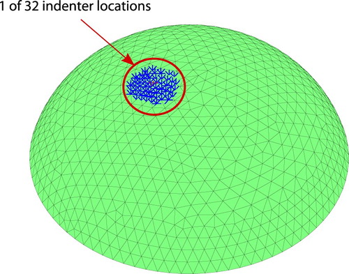
For each of the 32 locations, speckle data from the locating cylinders is extracted and we calculate the best-fit cylinder axis associated with that data (see Figure 15). The cylinder locations are projected to the surface of the ellipsoid model to obtain the indenter locations, which are used to identify the finite element mesh nodes on which to apply normal displacements (Figure 16).

Figure 15. Identifying indenter locations. (a) Speckled locating cylinders. (b) Point cloud from cylinder data acquisition with best-fit cylinder axis identified. (c) Indenter locations identified by projection to the surface of ellipsoid.

Figure 16. Finite element model of tissue phantom showing one of the indenter locations.

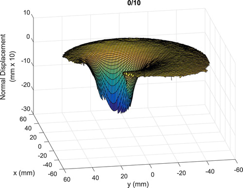
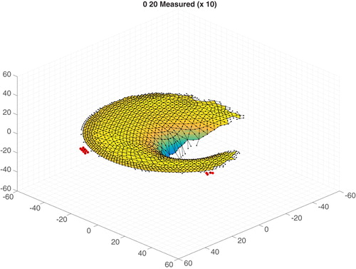
Next, we find the normal displacements for the tissue surface due to the indentations and verify the cylinder locations. We identify the surface normals from the ellipsoid fit. We extract the three-dimensional coordinates of the tissue surface from the initial contact (no cylinder) and the two indented images for each indentation location, and use the difference between the initial contact and indented data to generate the displacements. Taking the dot product of the surface normals with the displacement data allows us to calculate normal displacement data, and the normal displacements are averaged to create a preliminary normal displacement field for that indenter location as shown in Figure 17. Note the indenter partially blocks the camera's view so that surface data is not available at all locations, particularly close to the indenter head. Hence, the amplitude of the surface displacement shown in the figure is less than the 5 mm motion at the indenter head itself.

Figure 17. Preliminary surface normal displacements identified from measured data (note that the displacements are plotted at 10 times their actual values).

The verified measured data are interpolated to the finite element mesh nodes to create the final normal displacement data for our genetic algorithm. In this step nodal normals are calculated from the finite element mesh geometry. MATLAB's scatteredInterpolant function is used to interpolate the initial contact (before) and the two indented (after) data sets to the nodal locations. For each node in each data set, we check that there are at least four data points within a radius ‘rcheck’ to avoid interpolating between data points which are too widely spaced. A typical value of rcheck is 2.5 mm. In addition, for each node in each data set, we check that a simple estimate of the slope of the interpolated value is less than ‘max_deriv’ to avoid including data which contains unphysical peaks. A typical value of max_deriv is 1.4 mm/mm. Nodal locations which fail these checks are excluded from the inverse computation. The normal displacement at the nodes for the two indented cases is computed, and if the values are more than 0.5 mm (i.e. 10% of the indentation amplitude) apart this nodal location is excluded from the inverse computation. If the two normal indentations are within 0.5 mm then they are averaged and that node is marked to be included. The data sets are finally adjusted with a visual check to identify anomalous data not captured by the automated process. Figure 18 shows an example of the data. As mentioned before, all locations with missing data points are marked to be excluded from the inverse computation, and the final surface normal displacement data values are written.

Figure 18. Surface normal displacements projected to the mesh with anomalous point identification (selected anomalous points are highlighted. Displacement shown 10 times actual, all dimensions in mm).

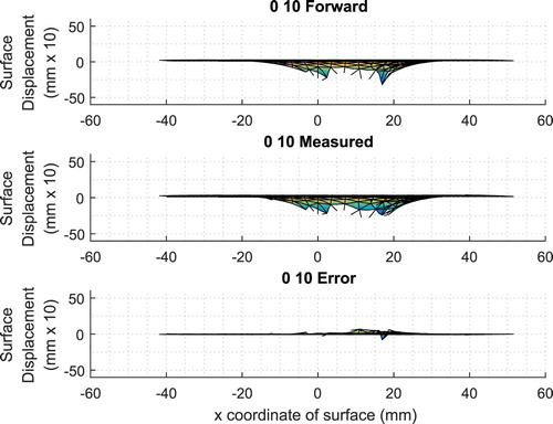
As a check, the finite element mesh and indenter locations are used to compute a tumour-free forward solution and that forward solution is compared with the measured data. Figure 19 shows a typical result for a single indenter location.

Figure 19. Typical comparison between the tumour-free forward-computed normal surface displacements and the measured data (first ‘0 10’ indenter location. Normal surface displacements shown 10 times actual).

Comparison of the experimentally measured surface data with the corresponding predictions from the forward solution to the finite element model allows us to estimate the errors (noise) inherent in our system. We computed the signal-to-noise ratio (SNR)⁷ for each of the 12 tumour-free phantoms relative to their corresponding forward finite element model. The average SNR over the 12 tumour-free phantoms was 13.0 dB and the values ranged from 12.3 to 13.9 dB. This SNR incorporates many potential sources of error, including: lack of normality in the indentations, inconsistencies in the indentation depth, errors in measuring the surface displacements, errors introduced in averaging and interpolating the measurements, approximations introduced by a linear material model, geometric inaccuracies introduced in fitting the surface data to an ellipsoid, and differences between the true boundary conditions and the finite element boundary conditions. We anticipate that this SNR information will be useful in informing the near-term algorithm improvements detailed in the section on Discussion and Future Work.

Once this data postprocessing and checking are complete, the finite element data and the processed experimental data for the normal displacements at the nodes are used as input to the GA/FEM algorithm described in Section 3.

5. Results

The GA/FEM returns the ‘best’ material distribution (among the allowed clumps). Recall that best material distribution is the one that has the lowest Cost (see Equation 1(1) $\text{Cost}=\frac{\delta }{{\delta }_{tf}}+w\frac{R_{tumour}}{R_{entire}}.$(1) ) and that the Cost balances the fit to the measured data and the penalty on large tumours. We seek a single w that works for all cases. We ran each set of experimental data with a weighting factor w=0.12.

We tested 12 samples without a tumour and 14 samples with a tumour. In all cases, the algorithm correctly identified the presence or absence of a tumour.

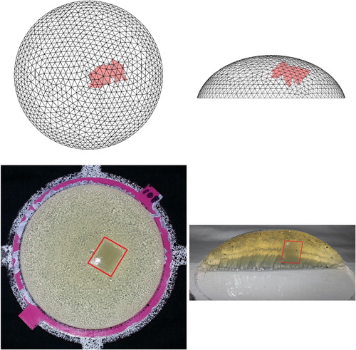
Figure 20 shows a typical result, for the tumour-containing phantom tested on 2017/03/24 with w=0.12. The top views show that the algorithm gives a very reasonable estimate of the location of the tumour in the tissue phantom. In addition, the side views indicate that the location of the tumour in the computational estimate is consistent with the location in the tissue phantom (midway between the top surface and the bottom surface). Since this procedure is envisioned as a screening tool only, the precise location or size of the tumour is not a major concern. Note, however, that the method inherently predicts the tumour location in three-dimensions and the top and side images are merely two views of a truly three-dimensional stiffness map.

Figure 20. Typical computational and experimental result (Top row: computational, Bottom row: experimental. w=0.12. Data taken on 2017/03/24).

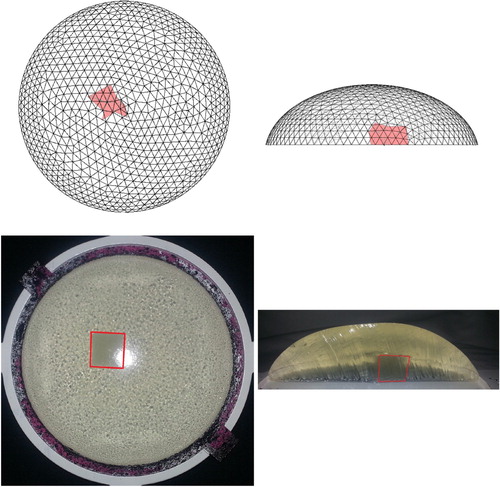
It is difficult to quantify the precise locations of the tumours experimentally because this can only be determined by dissecting the samples, and the dissection process distorts the phantom geometry. However, we have some control over the initial placement of the tumours and we studied tumours at varying depths and angular locations within the phantom. Figure 21 shows a case that we anticipated would be particularly challenging – a centrally located tumour very close to the rigid tray. As indicated in the figure the algorithm identified the location of this deep tumour quite well.

Figure 21. Result for a centrally located tumour close to the rigid tray (Top row: computational, Bottom row: experimental. w=0.12. Data taken on 2017/08/05).

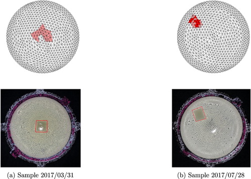
For all samples containing a tumour, the tumour locations identified by the algorithm were appropriate, as illustrated with top views for six more of the samples in Figures 22 and 23. Samples were tested that included tumours placed relatively near the top of the sample, midway between the top and bottom of the sample, and near the bottom of the sample.

Figure 22. Four results from phantoms containing a tumour using w=0.12. (a) Sample 2016/10/28 (b) Sample 2016/11/04 (c) Sample 2017/02/17 (d) Sample 2017/03/17

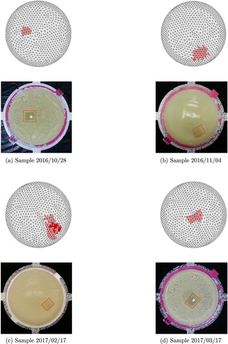
Figure 23. Two additional results from phantoms containing a tumour using w=0.12. (a) Sample 2017/03/31 (b) Sample 2017/07/28

Predicting the exact location is not critical in our application because the method is envisioned as a preliminary screening only. However, the ability to identify tumours that lie in a variety of locations is important. Due to space constraints, we have not shown both views of all samples tested, however, Table 1 gives geometric information on the relative locations and sizes of the tumours for all of the tumour-containing phantoms tested, as assessed from the dissected phantoms. Figure 24 will aid in interpreting the information in the table and defines the two scaling parameters R (the base radius of the phantom) and H (the vertical height of the phantom measured through the tumour centroid).

Figure 24. Definition of tumour location and size parameters listed in Table 1.

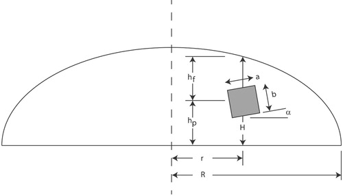
Table 1. Geometric information on the relative locations and sizes for tumours (parameters are defined in Figure 24. α reported to the nearest 5 degrees).

Sample Test date	r/R	H/R	$h_p/H$	$h_f/H$	a/R	b/R	α (degrees)	Shown in figure
2016/10/28	0.24	0.43	0.35	0.65	0.26	0.22	0	22
2016/11/04	0.52	0.45	0.40	0.60	0.27	0.27	0	22
2017/02/17	0.49	0.53	0.35	0.65	0.22	0.33	0	22
2017/03/17	0.18	0.57	0.32	0.68	0.19	0.28	0	22
2017/03/24	0.25	0.52	0.41	0.59	0.24	0.29	−10	20
2017/03/31	0.09	0.56	0.29	0.71	0.24	0.31	0	23
2017/07/14	0.25	0.59	0.41	0.59	0.31	0.22	−20
2017/07/15	0.36	0.56	0.41	0.59	0.24	0.28	−5
2017/07/22	0.47	0.52	0.52	0.48	0.25	0.22	15
2017/07/23	0.26	0.56	0.23	0.77	0.28	0.26	0
2017/07/28	0.50	0.50	0.38	0.62	0.30	0.25	15	23
2017/07/28b	0.27	0.54	0.27	0.73	0.28	0.27	0
2017/08/05	0.17	0.57	0.23	0.77	0.30	0.25	0	21
2017/08/05b	0.16	0.57	0.28	0.72	0.29	0.27	0

To understand this table, consider the sample from 3/24/2017 shown in Figure 20. That tumour has r/R=0.25, that is, it is about one-quarter of the way from the centre to the outer edge. In addition, that tumour is slightly closer to the plate ($h_p/H$=0.41) than it is to the free surface of the phantom ($h_f/H$=0.59). The deep tumour from 8/5/2017 shown in Figure 21 is closer to the centre (r/R=0.17) and much closer to the plate ($h_p/H$=0.23) than it is to the surface ($h_f/H$=0.77). Notice also that the tumours were not perfect cubes (only mass was controlled). As the table indicates, we successfully tested a wide variety of tumour locations.

We would like the algorithm to perform correctly for a wide range of w values. Because w penalizes the presence of tumours, as w becomes larger there is some value for which a sample containing a tumour will be reported as tumour-free. In addition, as w is decreased for tumour-free samples there is typically a value for which the fit to the data produces a spurious report of a tumour. As indicated previously w=0.12 worked for all of the tumour-free and tumour-containing samples tested. We can also identify the upper and lower bounds on w for each of the samples, as shown in Figure 25. Here the range for the 12 tumour-free samples is shown in the top half of the plot – each works correctly for some minimum w (occasionally the minimum w is zero ). The range for the 14 samples containing a tumour is displayed on the bottom half of the plot– each of those works up to some maximum value of w. For three of the tumour-containing samples the maximum is indicated clearly on the graph, but for many of them, the maximum is off the right side of the graph. Table 2 shows the numerical maximum values for each of the tumour-containing samples, since it varies widely. Between the minimum and maximum values of w is a rectangle which highlights the range from approximately w=0.11 to w=0.29 where all samples would be correctly identified. The value w=0.12 falls within this range.

Figure 25. Range of w for which each sample would be correctly identified, for all samples tested.

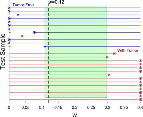
Table 2. Maximum w for correct identification of samples with tumours.

Sample test date	Upper bound for w
2016/10/28	0.3199
2016/11/04	0.2977
2017/02/17	0.4895
2017/03/17	0.7153
2017/03/24	0.4501
2017/03/31	1.4560
2017/07/14	0.3048
2017/07/15	0.4536
2017/07/22	0.5639
2017/07/23	0.6655
2017/07/28	0.5430
2017/07/28b	0.9651
2017/08/05	0.5218
2017/08/05b	0.8323

For these experiments, tumours as small as 2 g (approximately 1.3 cm cubes) can be detected in tissue phantoms. To put this in context, The American Joint Committee on Cancer [108] grades cancers in part by their tumour size. Breast cancer tumours less than 2 cm where cancer has not spread to other sites are collected into the lowest risk group for invasive cancers with a relative 5 year survival rate of 100% [109].

6. Discussion and future work

We have presented a genetic algorithm/finite element method for identifying tumours based only on surface displacement measurements. Experimental validation of the technique with 180 g gelatin tissue phantoms was able to correctly identify the presence or absence of 2 g tumours in 12 tumour-free phantoms and 14 tumour-containing phantoms. These results are promising but clearly, a great deal of work remains to be done before the method could be applied as a clinical screening tool.

In the near future, we will extend the method to include force measurements in the experiment and the computational algorithm. Displacement measurements have the advantage that they are not affected by the stiffness of the healthy tissues (only by the ratio of the healthy and cancerous tissue stiffnesses). However, the widely used manual palpation process depends primarily on forces. We anticipate that a combination of force and displacement measurements could be most effective for our stiffness mapping approach.

Additionally, we will use the existing experimental data to explore other approaches to the Cost function. For the fit to the data, rather than the one-norm of displacements we currently use, perhaps a two-norm for displacements or the signal-to-noise ratio between the measured data and the FEM might be more effective. Similarly, we have sought a single w for all cases but, while it has been successful here, inverse problems generally use a criteria based on the balance between the first and second terms to choose w and we hope to explore that question.

Near-term plans also include revisiting our initial computational simulations [5] to develop a computational simulation test-bed to identify algorithm and experimental improvements. Our initial simulations employed different indentation patterns than those we explored experimentally. Additionally, the experiment naturally cannot obtain data in certain locations and had different noise levels than in the original simulation. We will revisit the simulations and ensure that they correlate well with the current experimental setup. Then we will use this computational test-bed to explore questions such as the influence of different indentation patterns/sizes, possible optimization of indentation patterns, and identifying the most important regions on the surface for data collection.

These represent near-term explorations where many factors are still tightly controlled. However, it is certainly true that if the method fails under these conditions it is unsuitable, while if it succeeds then we have a good foundation from which to validate/refine/improve the method and expand its range of applicability. Ultimately many other factors that were tightly controlled in these preliminary validations will need to be examined including breast size and shape, tumour stiffness variations and healthy tissue inhomogeneities, as well as examination and computation time.

Breast size and shape will certainly play a role in our ability to map tumours and we will need to examine the algorithm's performance over a much wider range of breast geometries. There is nothing in the method that restricts the size of the breast model, but the distance from the tumour to the surface where measurements occur will certainly be a limiting factor and hence we would like to improve the sensitivity of the method (following our near-term plans) before attempting larger domains. Non-ellipsoidal breast shapes can be easily accommodated by the computations but it will ultimately be necessary to create algorithms to generate meshes for these more general geometries. Preliminary aspects of these examinations can occur with the computational simulation test-bed but experimental validation will be critical.

The relative stiffnesses in the tumours and the healthy tissue, as well as inhomogeneities in the tissues, will have an effect on mapping ability⁸. In previous work [111] we used computational simulations to study the effect of mismatches between the stiffness assumptions incorporated in the algorithm and the stiffnesses in the computational ‘experiment’. In addition, we examined the effect of lowering the relative stiffness between the cancerous and healthy tissues and allowing heterogeneities in the healthy tissue stiffness. The method was moderately robust to these variations. These studies will need to be revisited as we refine the approach, particularly as we add force information. The computational approach we use is not restricted to only two material properties– any number of different values may be coded into the chromosome – but because the search space is smaller the algorithm may perform better with two approximate properties than with many more precise values. The computational test-bed will once again provide valuable preliminary results that can be validated experimentally.

We envision that the total examination time and computation time would need to be reduced before the method could be used clinically, but both of those reductions seem feasible. Currently, we hold the indentations for at least 15 s and take two readings at each of 32 locations. With this 15 s hold the test takes a minimum of 16 min per breast. However, the 15 s hold is a conservative estimate of the time required to establish quasi-static conditions in the gelatin and we anticipate that could be reduced for actual breast tissue. Ultimately, automation in the data postprocessing will decrease the time to prepare the data for the algorithm. The genetic algorithm allows for an easy reduction in the total computing time as individual processors become faster and less expensive– in fact, one of the major reasons for choosing a genetic algorithm is that the computation time for this approach scales inversely with the number of processors. While the current wall-clock time for four processor nodes is 3.5 h, if we choose (even today) to run on eight nodes the wall-clock time drops to 1.75 h. The most recent upgrade to the Stampede computers reduced the computing time required for our analysis by a factor of 2.3 times and we anticipate that trend will continue. In addition, there are a number of algorithm efficiencies associated with mesh generation, memory use, and convergence detection that we plan to explore in the future. Hence, we believe that both the physical testing time and computational time limitations can ultimately be addressed.

As mentioned earlier, our preliminary results are promising but clearly, a great deal of work remains to be done before the method could be applied as a clinical screening tool.

Acknowledgments

We wish to thank Michael Insana (University of Illinois) for his advice and support. We also wish to acknowledge the contributions of our many other undergraduate researchers to the success of this project: Matthew Billingsley, Matthew Conrad, Emily Cottingham, Caitlin Douglas, Robert Fleishel, Wanli He, Tressa Lauer, Haley O'Neil, Gustavo Romo, Brendan Smyth, Griffin Steffy, James Tumavich, and Jiaojiao Wang. We also wish to thank HS, Inc of Oklahoma City, OK (www.hsfoodservers.com) for their gracious support of our work through an in-kind donation of tissue phantom molds.

Disclosure statement

No potential conflict of interest was reported by the authors.

Additional information

Funding

This material is based upon work supported by the National Science Foundation (Division of Electrical, Communications and Cyber Systems) [grant number ECCS-1306808]. This work used the Extreme Science and Engineering Discovery Environment (XSEDE), which is supported by National Science Foundation (Office of Advanced Cyberinfrastructure) [grant number ACI-1548562] (www.xsede.org). Resources were obtained through the Texas Advanced Computing Center (TACC) at the University of Texas at Austin (www.tacc.utexas.edu).

Notes

1. A genetic algorithm was chosen because it is a gradient-free optimization, easily incorporates constraints on material properties, allows an arbitrary choice of fitness function, and is easily parallelized.

2. Germall Plus Liquid, Crafter's Choice.

3. IMUSA 10-oz Multicolor Salsa Dish.

4. For our purposes, St. Venant's principle [107] means that the exact shape of the tumour does not affect the surface deflections measured at a distance from the tumour. Thus, any similarly sized tumour of the same stiffness would produce the same result.

5. McMaster-Carr 5/8“x 3/32“ Contact Points for Dial Indicator, #20625A421.

6. Speckles were made with Black Satin Krylon Fusion for Plastic spray paint.

7. We define the signal-to-noise ratio for a single indenter location as ${SNR}_i=20{\log }_{10}\left(\frac{\parallel forward{\parallel }_2}{\parallel forward-measured{\parallel }_2}\right)$ where forward is the nodal solution from the forward computation and measured is the processed experimental data for the normal displacements at the nodes. The SNR is given as the mean of the ${SNR}_i$ values over the 32 indenter locations.

8 Microcalcifications, which in certain configurations may be a sign of early breast cancer [110], would not be detected by this stiffness mapping approach.

Appendix. Details of the cost function calculation

Recall that we assign the fitness of each individual based on its ‘Cost’: $\text{Cost}=\frac{\delta }{{\delta }_{tf}}+w\frac{R_{tumour}}{R_{entire}}.$ δ is the sum of absolute errors between individual's normal displacements and the measured normal displacements, summed over all indentation sites. More precisely, let $f_{is}$ be the normal displacement calculated in the finite element solution at node i on the tissue surface for indentation site s, and let $d_{is}$ be the measured normal displacement interpolated to that same nodal location and indentation site. Then we calculate (A1) $\delta =\sum _{s=1}^S\sum _{i=1}^P|f_{is}-d_{is}|$(A1) where S is the number of indentation sites (32 in our experiments) and P is the number of surface points on the finite element mesh with valid experimental data. If there is no valid experimental data at a nodal location then that nodal location is not included in the error calculation (review the discussion in Section 4). ${\delta }_{tf}$ is the value of δ for a tumour-free individual.

To calculate $R_{entire}$ we first find the coordinates of the centroid of the entire domain. This can be done on an element-by-element basis: (A2) $x_c=\frac{{\displaystyle \sum _{i=1}^N{x}_{ci}{V}_i}}{{\displaystyle \sum _{i=1}^N{V}_i}},$(A2) where $x_c$ is the x-centroid of the domain, N is the number of volume elements in the finite element mesh, $x_{ci}$ is the x coordinate of the centroid of element i, and $V_i$ is the volume of element i. We make a similar calculation for $y_c$ and $z_c$. Next, we find the effective radius of the elements in the domain: (A3) $R_{entire}=\frac{{\displaystyle \sum _{i=1}^N{V}_i\sqrt{(x_{ci}-x_c{)}^2+(y_{ci}-y_c{)}^2+(z_{ci}-z_c{)}^2}}}{{\displaystyle \sum _{i=1}^N{V}_i}}.$(A3) $R_{tumour}$ is calculated analogously to $R_{entire}$, except that only cancerous elements are included in the summation: (A4) $x_{tc}=\frac{{\displaystyle \sum _{j=1}^M{x}_{cj}{V}_j}}{{\displaystyle \sum _{j=1}^M{V}_j}}.$(A4) Here $x_{tc}$ is the x coordinate of the tumour centroid and M is the total number of cancerous elements. The calculation for the effective radius of the tumour is also carried out by summing only over the cancerous elements: (A5) $R_{tumour}=\frac{{\displaystyle \sum _{j=1}^M{V}_j\sqrt{(x_{cj}-x_{tc}{)}^2+(y_{cj}-y_{tc}{)}^2+(z_{cj}-z_{tc}{)}^2}}}{{\displaystyle \sum _{j=1}^M{V}_j}}.$(A5)

References

- Breast cancer screening for women at average risk. https://ww5.komen.org/BreastCancer/BreastCancerScreeningforWomenatAverageRisk.html; 2018.
- American cancer society recommendations for the early detection of breast cancer. https://www.cancer.org/cancer/breast-cancer/screening-tests-and-early-detection.html; 2018.
- Samani A, Zubovits J, Plewes D. Elastic moduli of normal and pathological human breast tissues: an inversion-technique-based investigation of 169 samples. Phys Med Biol. 2007;52:1565–1576.
- Greenleaf JF, Fatemi M, Insana M. Selected methods for imaging elastic properties of biological tissues. Annu Rev Biomed Eng. 2003;5:57–78.
- Olson L, Throne R. Early detection of breast cancer through an inverse problem approach to stiffness mapping. Inverse Probl Sci Eng. 2013;21:314–338.
- Doyley MM. Model-based elastograpy: a survey of approaches to the inverse elasticity problem. Phys Med Biol. 2012;57:R35–R73.
- Parker KJ, Doyley MM, Rubens DJ. Imaging the elastic properties of tissue: the 20 year perspective. Phys Med Biol. 2011;56:1–29.
- Babniyi OA, Oberai AA, Barbone PE. Recovering vector displacement estimates in quasi-static elastography using sparse relaxation of the momentum equation. Inverse Probl Sci Eng. 2017;25(3):326–362.
- Babniyi OA, Oberai AA, Barbone PE. Direct error in constitutive equation formulation for plane stress inverse elasticity problem. Comput Methods Appl Mech Eng. 2017;314:3–18.
- Albocher U, Barbone PE, Richards MS, et al. Approaches to accommodate noisy data in the direct solution of inverse problems in incompressible plane strain elasticity. Inverse Probl Sci Eng. 2014;22(8):1307–1328.
- Albocher U, Barbone PE, Oberai AA. Uniqueness of inverse problems of isotropic incompressible three-dimensional elasticity. J Mech Phys Solids. 2014;73:55–68.
- Tyagi M, Goenezen S, Barbone PE, et al. Algorithm for quantitative quasi-static elasticity imaging using force data. Int J Numer Method Biomed Eng. 2014;30:1421–1436.
- Goenezen S, Dord JF, Sink Z, et al. Linear and nonlinear elastic modulus imaging: an application to breast cancer diagnosis. IEEE Trans Med Imaging. 2012;31(8):1628–1637.
- Goenezen S, Barbone P, Oberai AA. Solution of the nonlinear elasticity imaging inverse problem: the incompressible case. Comput Methods Appl Mech Eng. 2011;200:1406–1420.
- Richards MS, Barbone PE, Oberai AA. Quantitative three-dimensional elasticity imaging from quasi-static deformation: a phantom study. Phys Med Biol. 2009;54:757–779.
- Oberai AA, Gokhale NH, Goenezen S, et al. Linear and nonlinear elasticity imaging of soft tissue in vivo: demonstration of feasibility. Phys Med Biol. 2009;54:1191–1207.
- Rivas C, Barbone PE, Oberai AA. Divergence of finite element formulations for inverse problems treated as optimization problems. J Phys. 2008;135(012088):1–8.
- Gokhale NH, Barbone PE, Oberai AA. Solution of the nonlinear elasticity imaging inverse problem: the compressible case. Inverse Probl. 2008;24(045010):1–26.
- Barbone PE, Oberai AA. Elastic modulus imaging: some exact solutions of the compressible elastography inverse problem. Phys Med Biol. 2007;52:1577–1593.
- Barbone PE, Gokhale NH. Elastic modulus imaging: on the uniqueness and nonuniqueness of the elastography inverse problem in two dimensions. Inverse Probl. 2004;20:283–296.
- Oberai AA, Gokhale NH, Feijoo GR. Solution of inverse problems in elasticity imaging using the adjoint method. Inverse Probl. 2003;19:297–313.
- Oberai AA, Gokhale NH, Doyley MM, et al. Evaluation of the adjoint equation based algorithm for elasticity imaging. Phys Med Biol. 2004;49:2955–2974.
- Shore SW, Barbone PE, Oberai AA, et al. Transversely isotropic elasticity imaging of cancellous bone. J Biomech Eng. 2011;133:1–11.
- Ferreira ER, Oberai AA, Barbone PE. Uniqueness of the elastography inverse problem for incompressible nonlinear planar hyperelasticity. Inverse Probl. 2012;28:1–25.
- Park E, Maniatty AM. Shear modulus reconstruction in dynamic elastography: time harmonic case. Phys Med Biol. 2006;51:3697–3721.
- Park E, Maniatty AM. Finite element formulation for shear modulus reconstruction in transient elastography. Inverse Probl Sci Eng. 2009;17(5):605–626.
- McLaughlin JR, Zhang N, Manduca A. Calculating tissue shear modulus and pressure by 2D log-elastographic methods. Inverse Probl. 2010;26(085007):1–25.
- Lin K, McLaughlin J, Zhang N. Log-elastographic and non-marching full inverseion schemes for shear modulus recovery from single frequency elastographic data. Inverse Probl. 2009;25(075004):1–24.
- Lin K, McLaughlin J. An error estimate on the direct inversion model in shear stiffness imaging. Inverse Probl. 2009;25(075003):1–19.
- McLaughlin J, Renzi D. Shear wave speed recovery in transient elastography and supersonic imaging using propagating fronts. Inverse Probl. 2006;22:681–706.
- McLaughlin J, Renzi D. Using level set based inversion of arrival times to recover shear wave speed in transient elastography and supersonic imaging. Inverse Probl. 2006;22:707–725.
- Alizad A, Wold LE, Greenleaf JF, et al. Imaging mass lesions by vibro-acoustography: modelling and experiments. IEEE Trans Med Imaging. 2004;23(9):1087–1093.
- Brigham JC, Aquino W, Mitri FG, et al. Inverse estimation of viscoelastic material properties for solid immersed in fluids using vibroacoustic techniques. J Appl Phys. 2007;101:1–14.
- Zhang X, Zeraati M, Kinnick RR, et al. Vibration mode imaging. IEEE Trans Med Imaging. 2007;26(6):843–852.
- Mitri FG, Davis BJ, Alizad A, et al. Prostate cryotherapy monitoring using vibroacoustography: preliminary results of an ex-vivo study and technical feasibility. IEEE Trans Biomed Eng. 2008;55(11):2584–2592.
- Amador C, Urban MW, Chen S, et al. Shear elastic modulus estimation from indentation and SDUV on gelatin phantoms. IEEE Trans Biomed Eng. 2011;58(6):1706–1714.
- Amador C, Urban MW, Chen S, et al. Loss tangent and complex modulus estimated by acoustic radiation force creep and shear wave dispersion. Phys Med Biol. 2012;57:1263–1282.
- Urban MW, Chalek C, Kinnick RR, et al. Implementation of vibro-acoustography on a clinical ultrasound system. IEEE Trans Ultrason Ferroelectr Freq Control. 2011;58(6):1169–1181.
- Perrinez PR, Kennedy FE, Van Houten EEW, et al. Modeling of soft poroelastic tissue in time-harmonic MR elastography. IEEE Trans Biomed Eng. 2009;56(3):598–608.
- Perreard IM, Pattison AJ, Doyley M, et al. Effects of frequency- and direction-dependent elastic materials on linearly elastic MRE image reconstructions. Phys Med Biol. 2010;55:6801–6815.
- Eskandari H, Salcudean SE, Rohling R, et al. Real-time solution of the finite element inverse problem of viscoelasticity. Inverse Probl. 2011;27(085002):1–16.
- Guo Z, You S, Wan X, et al. A FEM-based direct method for material reconstruction inverse problem in soft tissue elastography. Comput Struct. 2010;88:1459–1468.
- Eskandari H, Goksel O, Salcudean SE, et al. Bandpass sampling of high-frequency tissue motion. IEEE Trans Ultrason Ferroelectr Freq Control. 2011;58(7):1332–1343.
- Doyley MM, Srinivasan S, Dimidenko E, et al. Enhancing the performance of model-based elastography by incorporating additional a priori information in the modulus reconstruction process. Phys Med Biol. 2006;51:95–112.
- Fehrenbach J, Masmoudi M, Souchon R, et al. Detection of small inclusions by elastography. Inverse Probl. 2006;22:1055–1069.
- Harrigan TP, Konofagu EE. Estimation of material elastic moduli in elastography: a local method, and an investigation of poisson's ratio sensitivity. J Biomech. 2004;37:1215–1221.
- Liew HL, Pinksy PM. Recovery of shear modulus in elastography using an adjoint method with b-spline representation. Finite Elem Anal Des. 2005;41:778–799.
- Liu HT, Sun LZ, Wang G, et al. Analytic modeling of breast elastography. Med Phys. 2003;30(9):2340–2349.
- Liu Y, Sun LZ, Wang G. Tomography-based 3-D anisotropic elastography using boundary measurements. IEEE Trans Med Imaging. 2005;24(10):1323–1333.
- Miga MI. A new approach to elastography using mutual information and finite elements. Phys Med Biol. 2003;48:467–480.
- Ou JJ, Ong RE, Yankeelov TE, et al. Evaluation of 3d modality-independent elastography for breast imaging: a simulation study. Phys Med Biol. 2008;53:147–163.
- Samani A, Bishop J, Plewes DB. A constrained modulus reconstruction technique for breast cancer assessment. IEEE Trans Med Imaging. 2001;20(9):877–885.
- Plewes DB, Bishop J, Samani A, et al. Visualization and quantification of breast cancer biomechanical properties with magnetic resonance elastography. Phys Med Biol. 2000;45:1591–1610.
- Sarvazyan AP, Rudenko OV, Swanson SD, et al. Shear wave elasticity imaging: a new ultrasonic technology of medical diagnostics. Ultrasound Med Biol. 1998;24(9):1419–1435.
- Sinkus R, Tanter M, Xydeas T, et al. Viscoelastic shear properties of in vivo breast lesions measured by MR elastography. Magn Reson Imaging. 2005;23:159–165.
- Sridhar M, Liu J, Insana MF. Viscoelasticity imaging using ultrasound: parameters and error analysis. Phys Med Biol. 2007;52:2425–2443.
- Thitaikumar A, Mobbs LM, Kraemer-Chant CM, et al. Breast tumor classification using axial shear strain elastography: a feasibility study. Phys Med Biol. 2008;53:4809–4823.
- Van Houten EEW, Doyley MM, Kennedy FE, et al. Initial in vivo experience with steady-state subzone-based MR elastography of the human breast. J Magn Reson Imaging. 2003;17:72–85.
- Van Houten EEW, vR Viviers D, McGarry MD, et al. Subzone based magnetic resonance elastography using a rayleigh damped material model. Med Phys. 2011;38(4):1993–2004.
- Washington CW, Miga MI. Modality independent elastography (MIE): a new approach to elasticity imaging. IEEE Trans Med Imaging. 2004;23(9):1117–1128.
- Zhu Y, Hall TJ, Jiang J. A finite-element approach for young's modulus reconstruction. IEEE Trans Med Imaging. 2003;22(7):890–901.
- Wellman PS. Tactile imaging. PhD Thesis, Harvard University. 1999;.
- Wellman PS, Dalton EP, Krag D, et al. Tactile imaging of breast masses. Arch Surg. 2001;136:204–208.
- Kaufman CS, Jacobsen L, Bachman BA, et al. Digital documentation of the physical examination: moving the clinical breast exam to the electronic medical record. Am J Surg. 2006;192(4):444–449.
- Weiss RE, Hartanto V, Perrotti M, et al. In vitro trial of the pilot prototype of the prostate mechanical imaging system. Urology. 2001;58(6):1059–1063.
- Niemczyk P, Cummings KB, Sarvazyan AP, et al. Correlation of mechanical imaging and histopathology of radical prostatectomy specimens: a pilot study for detecting breast cancer. J Urol. 1998;160:797–801.
- Sallaway L, Magee S, Shi J, et al. Detecting solid masses in phantom breast using mechanical indentation. Exp Mech. 2014;54:935–942.
- Kearney TJ, Airpetian A, Sarvazyan A. Tactile breast imaging to increase the sensitivity of breast examination. J Clin Oncol. 2004;22(14S):1037.
- Helvie MA, Carson PL, Saravazyan A, et al. Mechanical imaging of the breast: a pilot trial. Ultrasound Med Biol. 2003;29(5S):S112.
- Egorov V, Tsyuryupa S, Kanilo S, et al. Soft tissue elastometer. Med Eng Phys. 2008;30:206–212.
- Egorov V, Sarvazyan AP. Mechanical imaging of the breast. IEEE Trans Med Imaging. 2008;27(9):1275–1287.
- Egorov V, Kearney T, Pollak SB, et al. Differentiation of benign and malignant breast lesions by mechanical imaging. Breast Cancer Res Treat. 2009;118(1):67–80.
- Egorov V, van Raalte H, Sarvazyan AP. Vaginal tactile imaging. IEEE Trans Biomed Eng. 2010;57(7):1736–1744.
- Sarvazyan A, Egorov V. Mechanical imaging – a technology for 3-d visualization and characterization of soft tissue abnormalities. a review. Curr Med Imaging Rev. 2012;8(1):64–73.
- van Raalte H, Egorov V. Characterizing female pelvic floor conditions by tactile imaging. Int Urogynecological J. 2015;26:607–609.
- Peterson J. Introduction to suretouch for clinicians. age. 2017;5(6):7–11. https://sureincus/physician-introduction-1/.
- Kaufman CS, Son JS, Yered E, et al. Clinical studies of palpation imaging of the breast on over 1000 patients. 2014 San Antonio Breast Cancer Symposium. 2014;P1-02-09.
- Xu X, Gifford-Hollingsworth C, Sensenig R, et al. Breast tumor detection using piezoelectric fingers: first clinical report. J Am Coll Surg. 2013;216(6):1168–1173.
- Xu X, Chung Y, Brooks AD, et al. Development of arry piezoelectric fingers towards in-vivo breast tumor detection. Rev Sci Instrum. 2016;87:124301.
- Yegingil H, Shih WY, Shih WH. Probing model tumor interfacial properties using piezoelectric cantilevers. Rev Sci Instrum. 2010;81(095104):1–9.
- Yegingil H, Shih WY, Shih WH. All-electrical indentation shear modulus and elastic modulus measurement using a piezoelectric cantilever with a tip. J Appl Phys. 2007;101(054510):1–10.
- Yegingil H, Shih WY, Shih WH. Probing elastic tissue modulus and depth of bottom-supported inclusions in model tissues using piezoelectric cantilevers. Rev Sci Instrum. 2007;78(115101):1–6.
- Szewczyk ST, Shih WY, Shih WH. Palpationlike soft-material elastic modulus measurement using piezoelectric cantilevers. Rev Sci Instrum. 2006;77(044302):1–8.
- Yen PL, Chen DR, Yeh KT, et al. Development of a stiffness measurement accessory for ultrasound in breast cancer diagnosis. Med Eng Phys. 2011;33(9):1108–1119.
- Hii AJH, Hann CE, Chase JG, et al. Fast normalized cross correlation for motion tracking using basis functions. Comput Methods Programs Biomed. 2006;82:144–156.
- Peters A, Milsant A, Rouze J, et al. Digital image-based elasto-tomography: proof of concept studies for surface based mechanical property reconstruction. JOSE Int J. 2004;47(4):1117–1123.
- Peters A, Wortmann S, Elliott R, et al. Digital image-based elasto-tomography: first experiments in surface based mechanical property estimation of gelatine phantoms. JOSE Int J. 2005;48(4):562–569.
- Peters A, Uwe-Berger H, Chase JG, et al. Digital image-based elasto-tomography: non-linear mechanical property reconstruction of homogeneous gelatine phantoms. Int J Inf Syst Sci. 2006;2(4):512–521.
- Peters A, Chase JG, Van Houten EEW. Digital image elasto-tomography: combinatorial and hybrid optimization algorithms for shape-based elastic property reconstruction. IEEE Trans Biomed Eng. 2008;55(11):2575–2583.
- Peters A, Chase JG, Van Houten EEW. Estimating elasticity in heterogeneous phantoms using digital image elasto-tomography. Med Biol Eng Comput. 2009;47:67–76.
- Hann CE, Chase JG, Chen X, et al. Strobe imaging system for digital image-based elasto-tomography breast cancer screening. IEEE Trans Ind Electron. 2009;56(8):3195–3202.
- Botterill T, Lotz T, Kashif A, et al. Reconstructing 3-d skin surface motion for the diet breast cancer screening system. IEEE Trans Med Imaging. 2014;33(4):1109–1118.
- Peters A, Chase JG, Houten EEWV. Digital image elasto-tomography: mechanical property estimation of silicone phantoms. Med Biol Eng Comput. 2008;46:205–212.
- Kashif AS, Lotz TF, Heeren AMW, et al. Separate modal analysis for tumor detection with a digital image elasto tomography (diet) breast cancer screening system. Med Phys. 2013;40(11):113503:1–113503:8.
- Krouskop TA, Wheeler TM, Kallel F, et al. Elastic moduli of breast and prostate tissues under compression. Ultrason Imaging. 1998;20:260–274.
- Samani A, Plewes D. An inverse problem solution for measuring the elastic modulus of intact ex vivo breast tissue tumours. Phys Med Biol. 2007;52:1247–1260.
- Mehrabian H, Campbell G, Samani A. A constrained reconstruction technique of hyperelasticity parameters for breast cancer assessment. Phys Med Biol. 2010;55:7489–7508.
- O'Hagan JJ, Samani A. Measurement of the hyperelastic properties of 44 pathological ex vivo breast tissue samples. Phys Med Biol. 2009;54:2257–2569.
- O'Hagan JJ, Samani A. Measurement of the hyperelastic properties of tissue slices with tumour inclusion. Phys Med Biol. 2008;53:7087–7106.
- Valentin J. editor. Basic anatomical and physiological data for use in radiological protection: reference values. Ann ICRP. 2002;32:1–277.
- Westreich M. Anthropomorphic breast measurement: protocol and results in 50 women with aesthetically perfect breasts and clinical application. Plast Reconstr Surg. 1997;100:468–479.
- Smith DJ, Palin WE, Katch VL, et al. Breast volume and anthropomorphic measurements: normal values. Plast Reconstr Surg. 1986;78(3):331–335.
- Loughry CW, Sheffer DB, Price TE, et al. Breast volume measurement of 248 women using biostereometric analysis. Plast Reconstr Surg. 1986;80(4):553–558.
- Loughry CW, Sheffer DB, Price TE, et al. Breast volume measurement of 598 women using biostereometric analysis. Ann Plast Surg. 1989;22(5):380–385.
- Sussman TD. On the finite element analysis of incompressible solids [dissertation]. Massachusetts Institute of Technology; 1987.
- Samp M, Iovanac N, Nolte A. Sodium alginate toughening of gelatin hydrogels. ACS Biomaterials Science and Engineering. submitted.
- Love AE. A treatise on the mathematical theory of elasticity. 4th ed. Dover; 1944. First American Printing of the 1927 edition.
- American cancer society. http://www.cancer.org/; 2008.
- Ries LAG, Young JL, Keel GE, et al. editors. SEER survival monograph: cancer survival among adults: US SEER program, 1988-2001, patient and tumor characteristics. National Cancer Institute, SEER Program, NIH Pub. No. 07-6215; 2007. Http://seer.cancer.gov/publications/survival/.
- Breast calcifications. https://www.mayoclinic.org/symptoms/breast-calcifications/basics/definition/sym-20050834; 2018.
- Olson L, Throne R. Early detection of breast cancer through an inverse problem approach to stiffness mapping: 3D results and variations in properties. 12th US National Congress on Computational Mechanics. 2013.