Identification of thermal conductivity for orthotropic FGMs by DT-DRBEM and L-M algorithm

ABSTRACT

The differential transformation dual reciprocity boundary element method (DT-DRBEM) combined with the Levenberg–Marquardt (L-M) algorithm is proposed to identify the thermal conductivity for orthotropic functionally gradient materials (FGMs). The original governing equation of two-dimensional transient heat conduction problem is transformed into a time-independent and recursive form equation by the differential transformation method (DTM). The analog equation method is used to convert the partial differential equation to a standard thermal diffusion equation. Then, the DRBEM is applied to solve the direct problem and the measured temperature is obtained. After that, the L-M algorithm is used to minimize the objective function and recover the desired thermal conductivity. The DT-DRBEM is compared with the finite difference DRBEM (FD-DRBEM). The L-M algorithm is also compared with the conjugate gradient method (CGM). The influences of different initial guesses, number of measurement points and random errors on the inverse results are also investigated. The initial guesses have little effect on the number of iteration. With the increase of measurement points and with the decrease of measurement errors, the results are more accurate.

KEYWORDS:

• Inverse problem
• thermal conductivity
• functionally gradient materials
• differential transformation method
• DRBEM
• L-M algorithm

SUBJECT CLASSIFICATION CODES:

• 65M32
• 65M38

1. Introduction

Functionally gradient materials (FGMs) possess a smooth variation of material properties due to a gradual change in microstructural details. These characteristics make FGMs have better performance and advantages over the traditional composite materials [1–5]. The thermal conductivity of FGMs plays a very important role in determining the distribution of the temperature field. Therefore, accurate measurement and analysis of thermal conductivity are of great significance for the design, optimization, and engineering application of FGMs [6–11].

The boundary element method (BEM) is a robust numerical method for solving the linear and homogeneous heat conduction problems [12–14]. However, the BEM faces a serious challenge when solving non-linear, non-homogeneous and transient problems since there are domain integrals in the resulting integral equations. The dual reciprocity boundary element method (DRBEM) is an efficient method to transform the domain integral into the boundary integral [14–16].

For the transient heat conduction problem, a number of time-domain processing methods have been proposed [15–21], such as the finite difference method (FDM), the Laplace transform technique, etc. In 1986, Zhou [22] first put forward the differential transformation method (DTM). This method is based on Taylor expansion. It constructs an analytical solution in the form of a polynomial [23–25]. Moradi et al. [26] utilized the DTM to do the convection-radiation thermal analysis of triangular porous fins with temperature dependent thermal conductivity. Chu et al. [27] used the DTM and FDM to analyse a transient heat conduction problem.

In recent years, the inverse heat conduction problems have received widespread attention in engineering applications [28–33]. Flach et al. [6] estimated spatially varying thermal properties through a flash method type of experiment. Huang et al. [34] applied the conjugate gradient method (CGM) for estimating the unknown thermal conductivity and heat capacity. Mera et al. [35] proposed an alternating iterative BEM to estimate the unknown conductivity coefficients and the unknown boundary data for the two-dimensional heat conduction problem in an anisotropic medium. Shortly afterwards, Mera et al. [36] proposed another numerical algorithm to achieve this identification purpose based on the BEM and the least squares (LS) technique. Ardakani et al. [37] used the BEM and the particle swarm optimization (PSO) algorithm to identify the thermal conductivity of two-dimensional steady problems. Imani et al. [38] estimated the temperature dependent thermal conductivity and heat capacity based on a modified genetic algorithm. Hematiyan et al. [39] retrieved three-dimensional thermal conductivity of anisotropic media based on the BEM and the damped Gauss–Newton method. Kim et al. [40] determined the temperature dependent thermophysical properties of anisotropic composite material by the modified Newton method. Nedin et al. [9] identified the thermal conductivity coefficient and volumetric heat capacity of FGMs. Chen et al. [11] retrieved the space dependent thermal conductivity in a FGM hollow cylinder based on the CGM and the deviation principle. Mohebbi et al. [41,42] estimated the space and temperature dependent heat transfer coefficient and proposed a new method to solve the sensitivity coefficients matrix through derived expressions. Dulikravich et al. [43–45] assumed the analytical expression for continuously varying thermal conductivity and determined the spatial distribution of material properties by using the PSO algorithm or a hybrid of PSO and Broyden-Fletcher-Goldfarb-Shanno (BFGS) algorithms.

The Levenberg–Marquardt (L-M) algorithm [46] is a standard technique for non-linear least squares problems, widely adopted in a broad spectrum of disciplines. It can be regarded as a combination of gradient descent method [47] and the Gauss–Newton method [48]. Sawaf et al. [49] estimated temperature dependent thermal conductivity and specific heat capacity by using the L-M algorithm. Rodriguez-Quinonez et al. [50] used the L-M algorithm as a digital rectifier to adjust the non-linear variation and increase the measurement accuracy of the three-dimensional Rotational Body Scanner, and compared the CGM and quasi-Newton method. Cui et al. [51,52] applied the CGM, LS method and L-M algorithm, to identify the temperature dependent thermal conductivity based on the FDM. And the complex variable derivation method was used to solve the sensitivity matrix.

The purpose of this paper is to determine the unknown thermal conductivity. It is difficult to predict it if there is not a function expression. Because the derivatives of the thermal conductivity respect to space coordinates are essential for the inverse analysis. The problem is feasible if some priori information about the analytical variation of the thermal conductivity in space is given in advance. The identification of the thermal conductivity can be achieved by recovering the parameter for the specified analytical model.

For the transient heat conduction problems, the traditional FDM is often used to treat the derivative of temperature with respect to time. Although the FDM is simple, due to the effect of error accumulation and time step, the calculation results are usually inaccurate. So the DTM is proposed to avoid the weakness in this paper. The differential transformation DRBEM (DT-DRBEM) replaces the finite difference DRBEM (FD-DRBEM) to solve the direct heat conduction problem. For the inverse problem, the CGM and the L-M algorithm are common methods, but the convergence rate of the CGM is slow. So the L-M algorithm is used to improve the computation efficiency.

In this paper, the DT-DRBEM combined with the L-M algorithm is proposed for estimating the thermal conductivity in orthotropic FGMs. This paper is organized as follows: the theory of the DT-DRBEM in FGMs is introduced in Section 2. The operation principle of the L-M algorithm is described in Section 3, and the implementation processes are given. In Section 4, some examples are given to verify the proposed method, and Section 5 contains some conclusion remarks.

2. Direct problem

2.1. Differential transformation method

Assume that $x\left(\tau \right)$ is an arbitrary function and let $\tau ={\tau }_0$ represents any point in the domain $D$. The function $x\left(\tau \right)$ is then represented by a power series whose centre is located at ${\tau }_0$. The differential transform of the function $x\left(\tau \right)$ is (1) $X\left(m\right)=\frac{1}{m!}{\left[\frac{{\mathrm{d}}^{m}x\left(\tau \right)}{\mathrm{d}{\tau }^m}\right]}_{\tau ={\tau }_0},$(1) in which $x\left(\tau \right)$ is an original function and $X\left(m\right)$ is the transformed function. The inverse transformation (2) $x\left(\tau \right)=\sum _{m=0}^{\mathrm{\infty }}{\left(\tau -{\tau }_0\right)}^{m}X\left(m\right).$(2)

In fact, Equation (2) can be also understood as the Taylor series expansion of function $x\left(\tau \right)$ at ${\tau }_0$. The fundamental operations of the DTM are listed in Table 1 [23,24,26].

Table 1. The fundamental operations of the DTM.

Original function	Transformed function
$x\left(\tau \right)=f\left(\tau \right)+g\left(\tau \right)$	$X\left(m\right)=F\left(m\right)+G\left(m\right)$
$x\left(\tau \right)={\displaystyle \frac{\mathrm{d}f\left(\tau \right)}{\mathrm{d}\tau }}$	$X\left(m\right)=\left(m+1\right)F\left(m+1\right)$
$x\left(\tau \right)={\displaystyle \frac{{\mathrm{d}}^{n}f\left(\tau \right)}{\mathrm{d}{\tau }^n}}$	$X\left(m\right)={\displaystyle \frac{\left(m+n\right)!}{m!}}F\left(m+n\right)$
$x\left(\tau \right)=\exp \left(\lambda \tau \right)$	$X\left(m\right)={\displaystyle \frac{{\lambda }^m}{m!}}$
$x\left(\tau \right)={\tau }^r$	$X\left(m\right)=\delta \left(m-r\right)=\left\{\begin{array}{l}1,m=r\\ 0,otherwise\end{array}\right.$
$x\left(\tau \right)=f\left(\tau \right)g\left(\tau \right)$	$X\left(m\right)={\sum }_{n=0}^{m}F\left(n\right)G\left(m-n\right)$

Based on the basic principles of the DTM, for $\tau \in \left[{\tau }_n,{\tau }_{n+1}\right]\left(n\ge 0\right)$, assuming any function $u\left(\tau \right)$ can be written as follows (3) $u\left(\tau \right)=\sum _{m=0}^{\mathrm{\infty }}\frac{{\left(\tau -{\tau }_n\right)}^m}{{\left(\mathrm{\Delta }\tau \right)}^m}U\left(m\right).$(3)

Then the function $U\left(m\right)$ can be expressed as (4) $U\left(m\right)=\frac{{\left(\mathrm{\Delta }\tau \right)}^m}{m!}{\left[\frac{{\mathrm{d}}^{m}u\left(\tau \right)}{\mathrm{d}{\tau }^m}\right]}_{\tau ={\tau }_n},$(4) where $\mathrm{\Delta }\tau ={\tau }_{n+1}-{\tau }_n$.

2.2. Governing equation

The governing equation of two-dimensional transient heat conduction problem in orthotropic FGMs can be expressed as (5) $\frac{\mathrm{\partial }}{\mathrm{\partial }{x}_1}\left[{\lambda }_{11}\left(\mathbf{x}\right)\frac{\mathrm{\partial }t\left(\mathbf{x},\tau \right)}{\mathrm{\partial }{x}_1}\right]+\frac{\mathrm{\partial }}{\mathrm{\partial }{x}_2}\left[{\lambda }_{22}\left(\mathbf{x}\right)\frac{\mathrm{\partial }t\left(\mathbf{x},\tau \right)}{\mathrm{\partial }{x}_2}\right]=\rho c\frac{\mathrm{\partial }t\left(\mathbf{x},\tau \right)}{\mathrm{\partial }\tau },$(5) with the initial condition (6) $t\left(\mathbf{x},\tau \right){|}_{\tau =0}=t_0\left(\mathbf{x}\right),$(6) and the boundary conditions are given as (7) $\left\{\begin{array}{l}t\left(\mathbf{x},\tau \right)=\overline{t}\left(\mathbf{x},\tau \right),\mathbf{x}\in {\mathrm{\Gamma }}_1\\ q\left(\mathbf{x},\tau \right)=\frac{\mathrm{\partial }t\left(\mathbf{x},\tau \right)}{\mathrm{\partial }\mathbf{n}}=\overline{q}\left(\mathbf{x},\tau \right),\mathbf{x}\in {\mathrm{\Gamma }}_2\end{array}\right..$(7)

In Equations (5–7), $\mathbf{x}=(x_1,x_2)$, $t\left(\mathbf{x},\tau \right)$ is the temperature of point $\mathbf{x}\in \mathrm{\Omega }$ at time $\tau$, ${\lambda }_{ii}\left(\mathbf{x}\right)$ is the space dependent thermal conductivity, $\rho$ is the density and $c$ is the specific heat, $t_0$ is a prescribed function. ${\mathrm{\Gamma }}_1\cup {\mathrm{\Gamma }}_2=\mathrm{\Gamma }$, ${\mathrm{\Gamma }}_1\cap {\mathrm{\Gamma }}_2=\mathrm{\varnothing }$, $\mathrm{\Gamma }=\mathrm{\partial }\mathrm{\Omega }$, $\mathrm{\partial }t\left(\mathbf{x},\tau \right)/\mathrm{\partial }\mathbf{n}$ signifies the normal derivative of $\mathrm{\partial }t\left(\mathbf{x},\tau \right)$, $\mathbf{n}$ is the unit outward normal to the boundary $\mathrm{\Gamma }$, $\overline{t}$ and $\overline{q}$ are prescribed temperature and heat flux history on corresponding boundary.

2.3. Recursive governing equation

In any time interval $\tau \in \left[{\tau }_n,{\tau }_{n+1}\right]\left(n\ge 0\right)$, the DTM is applied for Equation (5) to obtain the recursive governing equation. Let $u\left(\mathbf{x},\tau \right)=\mathrm{\partial }t\left(\mathbf{x},\tau \right)/\mathrm{\partial }\tau$, and using the Equation (4), the following equation can be obtained. (8) $U\left(m\right)=\frac{{\left(\Delta \tau \right)}^m}{m!}\frac{{\mathrm{\partial }}^{m}u\left(\mathbf{x},\tau \right)}{\mathrm{\partial }{\tau }^m}=\frac{m+1}{\Delta \tau }\frac{{\left(\Delta \tau \right)}^{m+1}}{\left(m+1\right)!}\frac{{\mathrm{\partial }}^{m+1}t\left(\mathbf{x},\tau \right)}{\mathrm{\partial }{\tau }^{m+1}}=\frac{m+1}{\Delta \tau }T\left(m+1\right),$(8) (9) $\rho cU\left(m\right)=\frac{\mathrm{\partial }}{\mathrm{\partial }{x}_1}\left[{\lambda }_{11}\left(\mathbf{x}\right)\frac{\mathrm{\partial }T\left(m\right)}{\mathrm{\partial }{x}_1}\right]+\frac{\mathrm{\partial }}{\mathrm{\partial }{x}_2}\left[{\lambda }_{22}\left(\mathbf{x}\right)\frac{\mathrm{\partial }T\left(m\right)}{\mathrm{\partial }{x}_2}\right].$(9)

Substituting Equation (8) into Equation (9), the recursive governing equation can be written as (10) $\frac{\mathrm{\partial }}{\mathrm{\partial }{x}_1}\left[{\lambda }_{11}\left(\mathbf{x}\right)\frac{\mathrm{\partial }T\left(m\right)}{\mathrm{\partial }{x}_1}\right]+\frac{\mathrm{\partial }}{\mathrm{\partial }{x}_2}\left[{\lambda }_{22}\left(\mathbf{x}\right)\frac{\mathrm{\partial }T\left(m\right)}{\mathrm{\partial }{x}_2}\right]=\theta T\left(m+1\right),$(10) where $\theta =\rho c\left(m+1\right)/\mathrm{\Delta }\tau$.

Similarly, the boundary conditions can be expressed as (11) $\left\{\begin{array}{l}T\left(m\right)=\overline{T}\left(m\right),\mathbf{x}\in {\mathrm{\Gamma }}_1\\ \mathrm{Q}\left(m\right)=\overline{\mathrm{Q}}\left(m\right),\mathbf{x}\in {\mathrm{\Gamma }}_2\end{array}\right..$(11)

2.4. Implement of the dual reciprocity method

Using the analog equation method, Equation (10) is reformulated as (12) $\frac{\mathrm{\partial }{\lambda }_{11}\left(\mathbf{x}\right)}{\mathrm{\partial }{x}_1}\frac{\mathrm{\partial }T\left(m\right)}{\mathrm{\partial }{x}_1}+{\lambda }_{11}\left(\mathbf{x}\right)\frac{{\mathrm{\partial }}^{2}T\left(m\right)}{\mathrm{\partial }{x_1}^2}+\frac{\mathrm{\partial }{\lambda }_{22}\left(\mathbf{x}\right)}{\mathrm{\partial }{x}_2}\frac{\mathrm{\partial }T\left(m\right)}{\mathrm{\partial }{x}_2}+{\lambda }_{22}\left(\mathbf{x}\right)\frac{{\mathrm{\partial }}^{2}T\left(m\right)}{\mathrm{\partial }{x_2}^2}=\theta T\left(m+1\right).$(12)

Extracting the differential operators of steady-state conduction in isotropic solids from Equation (12) and transposing it to the left-hand side [16], Equation (12) becomes (13) $\begin{array}{rl}\lambda \frac{{\mathrm{\partial }}^{2}T\left(m\right)}{\mathrm{\partial }{x_1}^2}+\lambda \frac{{\mathrm{\partial }}^{2}T\left(m\right)}{\mathrm{\partial }{x_2}^2}& =\left(\lambda -{\lambda }_{11}\left(\mathbf{x}\right)\right)\frac{{\mathrm{\partial }}^{2}T\left(m\right)}{\mathrm{\partial }{x_1}^2}+\left(\lambda -{\lambda }_{22}\left(\mathbf{x}\right)\right)\frac{{\mathrm{\partial }}^{2}T\left(m\right)}{\mathrm{\partial }{x_2}^2}\\ & -\frac{\mathrm{\partial }{\lambda }_{11}\left(\mathbf{x}\right)}{\mathrm{\partial }{x}_1}\frac{\mathrm{\partial }T\left(m\right)}{\mathrm{\partial }{x}_1}-\frac{\mathrm{\partial }{\lambda }_{22}\left(\mathbf{x}\right)}{\mathrm{\partial }{x}_2}\frac{\mathrm{\partial }T\left(m\right)}{\mathrm{\partial }{x}_2}+\theta T\left(m+1\right),\end{array}$(13) where $\lambda$ is the thermal conductivity in isotropic solids.

Equation (13) is rewritten as (14) $\lambda {\mathrm{\nabla }}^{2}T\left(m\right)=b,$(14) where (15) $\begin{array}{rl}b& =\left(\lambda -{\lambda }_{11}\left(\mathbf{x}\right)\right)\frac{{\mathrm{\partial }}^{2}T\left(m\right)}{\mathrm{\partial }{x_1}^2}+\left(\lambda -{\lambda }_{22}\left(\mathbf{x}\right)\right)\frac{{\mathrm{\partial }}^{2}T\left(m\right)}{\mathrm{\partial }{x_2}^2}\\ & -\frac{\mathrm{\partial }{\lambda }_{11}\left(\mathbf{x}\right)}{\mathrm{\partial }{x}_1}\frac{\mathrm{\partial }T\left(m\right)}{\mathrm{\partial }{x}_1}-\frac{\mathrm{\partial }{\lambda }_{22}\left(\mathbf{x}\right)}{\mathrm{\partial }{x}_2}\frac{\mathrm{\partial }T\left(m\right)}{\mathrm{\partial }{x}_2}+\theta T\left(m+1\right).\end{array}$(15)

Equation (14) can be multiplied by the fundamental solution of Laplace equation [14] and integrated over the domain. The following integral equation can be obtained (16) ${\int }_{\mathrm{\Omega }}\lambda {\mathrm{\nabla }}^{2}T\left(m\right)u^{\ast }\mathrm{d}\mathrm{\Omega }={\int }_{\mathrm{\Omega }}b{u}^{\ast }\mathrm{d}\mathrm{\Omega },$(16) where $u^{\ast }=\left(1/2\pi \right)\ln \left(1/r\right)$, $r=||\mathbf{x}-\mathbf{y}|{|}_2$ is the distance between source point $\mathbf{y}$ and field point $\mathbf{x}$.

Using Gauss’ divergence theorem, the left-hand side of Equation (16) can be expressed as (17) ${\int }_{\mathrm{\Omega }}\lambda {\mathrm{\nabla }}^{2}T\left(m\right)u^{\ast }\mathrm{d}\mathrm{\Omega }=-\lambda \left\{c\left(\mathbf{y}\right)T_{\mathbf{y}}\left(m\right)+{\int }_{\mathrm{\Gamma }}\frac{\mathrm{\partial }{u}^{\ast }}{\mathrm{\partial }\mathbf{n}}T\left(m\right)\mathrm{d}\mathrm{\Gamma }-{\int }_{\mathrm{\Gamma }}{u}^{\ast }\frac{\mathrm{\partial }T\left(m\right)}{\mathrm{\partial }\mathbf{n}}\mathrm{d}\mathrm{\Gamma }\right\},$(17) where $T_{\mathbf{y}}\left(m\right)$ denotes $T\left(m\right)$ at source point $\mathbf{y}$, the coefficient $c\left(\mathit{y}\right)$ depends on the smoothness of the boundary point $\mathbf{y}$.

For the right-hand side in Equation (16), the DRM is applied to transform the domain integral into the boundary integral. $b$ can be approximated as follows (18) $b\approx \sum _{j=1}^{N_T}{\alpha }^{j}f\left(\mathbf{x},{\mathbf{z}}_j\right),$(18) where $N_T=N_B+N_I$ is the total number of nodes, $N_B$ is the number of nodes on the boundary $\mathrm{\Gamma }$, $N_I$ is the number of internal nodes in the domain $\mathrm{\Omega }$. ${\alpha }^j$ is a set of unknown coefficients, $f\left(\mathbf{x},{\mathbf{z}}_j\right)$ is the radial basis function (RBF) and $\mathbf{x}$ represents field points, ${\mathbf{z}}_j$ is j-th collocation point of the DRM, respectively. The particular solutions ${\hat{T}}^j$ and the function $f\left(\mathbf{x},{\mathbf{z}}_j\right)$ are linked through the relation (19) $\lambda {\mathrm{\nabla }}^2{\hat{T}}^j=f\left(\mathbf{x},{\mathbf{z}}_j\right).$(19)

Substituting Equation (19) into Equation (18), Equation (18) can be written as (20) $b\approx \sum _{j=1}^{N_T}{\alpha }^j\left(\lambda {\mathrm{\nabla }}^2{\hat{T}}^j\right).$(20)

The RBF is expressed as [14] (21) $f\left(\mathbf{x},{\mathbf{z}}_j\right)=1+R+R^2.$(21)

Then, the particular solution ${\hat{T}}^j$ is obtained (22) ${\hat{T}}^j=\frac{R^2}{4}+\frac{R^3}{9}+\frac{R^4}{16},$(22) where (23) $R=\frac{1}{\sqrt{\lambda }}||\mathbf{x}-{\mathbf{z}}_j|{|}_2.$(23)

Substituting Equation (20) into Equation (16) and using Gauss’ divergence theorem similarly, the domain integral of the right-hand side in Equation (16) is transformed into a boundary integral. After that, combining Equation (17), a pure boundary integral equation can be obtained (24) $\begin{array}{rl}& c\left(\mathbf{y}\right)T_{\mathbf{y}}\left(m\right)+{\int }_{\mathrm{\Gamma }}\frac{\mathrm{\partial }{u}^{\ast }}{\mathrm{\partial }\mathbf{n}}T\left(m\right)\mathrm{d}\mathrm{\Gamma }-{\int }_{\mathrm{\Gamma }}{u}^{\ast }\frac{\mathrm{\partial }T\left(m\right)}{\mathrm{\partial }\mathbf{n}}\mathrm{d}\mathrm{\Gamma }\\ & =\sum _{j=1}^{N_T}{\alpha }^j\left\{c\left(\mathbf{y}\right){\hat{T}}_{\mathbf{y}}^j+{\int }_{\mathrm{\Gamma }}\frac{\mathrm{\partial }{u}^{\ast }}{\mathrm{\partial }\mathbf{n}}{\hat{T}}^j\mathrm{d}\mathrm{\Gamma }-{\int }_{\mathrm{\Gamma }}{u}^{\ast }\frac{\mathrm{\partial }{\hat{T}}^j}{\mathrm{\partial }\mathbf{n}}\mathrm{d}\mathrm{\Gamma }\right\},\end{array}$(24)

After discretizing the boundary into a series of $N_B$ elements, Equation (24) can be written as follows (25) $\begin{array}{rl}& c_i{T}_i\left(m\right)+\sum _{k=1}^{N_B}{H}_{ik}{T}_k\left(m\right)-\sum _{k=1}^{N_B}{G}_{ik}\frac{\mathrm{\partial }{T}_k\left(m\right)}{\mathrm{\partial }\mathbf{n}}\\ & =\sum _{j=1}^{N_T}{\alpha }^j\left(c_i{\hat{T}}_i^j+\sum _{k=1}^{N_B}{H}_{ik}{\hat{T}}_k^j-\sum _{k=1}^{N_B}{G}_{ik}\frac{\mathrm{\partial }{\hat{T}}_k^j}{\mathrm{\partial }\mathbf{n}}\right),\left(i=1,2,\cdots ,N_T\right),\end{array}$(25) and the Equation (25) can be expressed in a matrix form (26) $\mathbf{H}\mathbf{T}\left(m\right)-\mathbf{G}\mathbf{Q}\left(m\right)=\left(\mathbf{H}\hat{\mathbf{T}}-\mathbf{G}\hat{\mathbf{Q}}\right)\alpha .$(26)

The unknown coefficients $\alpha$ in Equation (26) can be obtained by (27) $\alpha ={\mathbf{F}}^{-1}\mathbf{b}=\left\{{\mathbf{K}}_1{\mathbf{T}}_{x_1{x}_1}\left(m\right)+{\mathbf{K}}_2{\mathbf{T}}_{x_2{x}_2}\left(m\right)-{\mathbf{P}}_1{\mathbf{T}}_{x_1}\left(m\right)-{\mathbf{P}}_2{\mathbf{T}}_{x_2}\left(m\right)+\theta \mathbf{T}\left(m+1\right)\right\},$(27) where ${\mathbf{F}}^{-1}$ is the inverse of $\mathbf{F}$. That is (28) $\mathbf{F}=\left[\begin{array}{cccc}f\left({\mathbf{x}}_1,{\mathbf{z}}_1\right)& f\left({\mathbf{x}}_1,{\mathbf{z}}_2\right)& \dots & f\left({\mathbf{x}}_1,{\mathbf{z}}_{N_T}\right)\\ f\left({\mathbf{x}}_2,{\mathbf{z}}_1\right)& f\left({\mathbf{x}}_2,{\mathbf{z}}_2\right)& \dots & f\left({\mathbf{x}}_2,{\mathbf{z}}_{N_T}\right)\\ \dots & \dots & \dots & \dots \\ f\left({\mathbf{x}}_{N_T},{\mathbf{z}}_1\right)& f\left({\mathbf{x}}_{N_T},{\mathbf{z}}_2\right)& \dots & f\left({\mathbf{x}}_{N_T},{\mathbf{z}}_{N_T}\right)\end{array}\right].$(28)

The matrices and vectors in Equation (27) can be expressed as follows (29) ${\mathbf{K}}_i=\left[\begin{array}{cccc}\lambda -{\lambda }_{ii}\left({\mathbf{x}}_1\right)& 0& \dots & 0\\ 0& \lambda -{\lambda }_{ii}\left({\mathbf{x}}_2\right)& \dots & 0\\ \dots & \dots & \dots & \dots \\ 0& 0& \dots & \lambda -{\lambda }_{ii}\left({\mathbf{x}}_{N_T}\right)\end{array}\right],\left(i=1,2\right),$(29) (30) ${\mathbf{T}}_{x_i{x}_i}={\left[\begin{array}{cccc}\frac{{\mathrm{\partial }}^2{T}^1\left(m\right)}{\mathrm{\partial }{x}_i^2}& \frac{{\mathrm{\partial }}^2{T}^2\left(m\right)}{\mathrm{\partial }{x}_i^2}& \dots & \frac{{\mathrm{\partial }}^2{T}^{N_T}\left(m\right)}{\mathrm{\partial }{x}_i^2}\end{array}\right]}^{\mathrm{T}},\left(i=1,2\right),$(30) (31) ${\mathbf{P}}_i=\left[\begin{array}{cccc}\frac{\mathrm{\partial }{\lambda }_{ii}\left({\mathbf{x}}_1\right)}{\mathrm{\partial }{x}_i}& 0& \dots & 0\\ 0& \frac{\mathrm{\partial }{\lambda }_{ii}\left({\mathbf{x}}_2\right)}{\mathrm{\partial }{x}_i}& \dots & 0\\ \dots & \dots & \dots & \dots \\ 0& 0& \dots & \frac{\mathrm{\partial }{\lambda }_{ii}\left({\mathbf{x}}_{N_T}\right)}{\mathrm{\partial }{x}_i}\end{array}\right],\left(i=1,2\right),$(31) (32) ${\mathbf{T}}_{x_i}={\left[\begin{array}{cccc}\frac{\mathrm{\partial }{T}^1\left(m\right)}{\mathrm{\partial }{x}_i}& \frac{\mathrm{\partial }{T}^2\left(m\right)}{\mathrm{\partial }{x}_i}& \dots & \frac{\mathrm{\partial }{T}^{N_T}\left(m\right)}{\mathrm{\partial }{x}_i}\end{array}\right]}^{\mathrm{T}},\left(i=1,2\right).$(32)

$T\left(m\right)$ is also approximated by the RBF (33) $T\left(m\right)\approx \sum _{j=1}^{N_T}{\gamma }^{j}f\left(\mathbf{x},{\mathbf{z}}_j\right),$(33) where ${\gamma }^j$ are unknown coefficients. Then, the first derivative of function $T\left(m\right)$ with respect to the coordinates $x_i$ in Equation (32)(32) ${\mathbf{T}}_{x_i}={\left[\begin{array}{cccc}\frac{\mathrm{\partial }{T}^1\left(m\right)}{\mathrm{\partial }{x}_i}& \frac{\mathrm{\partial }{T}^2\left(m\right)}{\mathrm{\partial }{x}_i}& \dots & \frac{\mathrm{\partial }{T}^{N_T}\left(m\right)}{\mathrm{\partial }{x}_i}\end{array}\right]}^{\mathrm{T}},\left(i=1,2\right).$(32) becomes (34) $\frac{\mathrm{\partial }T\left(m\right)}{\mathrm{\partial }{x}_i}\approx \sum _{j=1}^{N_T}{\gamma }^j\frac{f\left(\mathbf{x},{\mathbf{z}}_j\right)}{\mathrm{\partial }{x}_i},\left(i=1,2\right).$(34)

The coefficients ${\gamma }^j$ can be determined by Equation (33) and the first derivative of $T\left(m\right)$ is evaluated as follows (35) ${\mathbf{T}}_{x_i}\left(m\right)\approx {\mathbf{F}}_{x_i}{\mathbf{F}}^{-1}\mathbf{T}\left(m\right),$(35) where (36) ${\mathbf{F}}_{x_i}=\left[\begin{array}{cccc}\frac{\mathrm{\partial }f\left({\mathbf{x}}_1,{\mathbf{z}}_1\right)}{\mathrm{\partial }{x}_i}& \frac{\mathrm{\partial }f\left({\mathbf{x}}_1,{\mathbf{z}}_2\right)}{\mathrm{\partial }{x}_i}& \dots & \frac{\mathrm{\partial }f\left({\mathbf{x}}_1,{\mathbf{z}}_{N_T}\right)}{\mathrm{\partial }{x}_i}\\ \frac{\mathrm{\partial }f\left({\mathbf{x}}_2,{\mathbf{z}}_1\right)}{\mathrm{\partial }{x}_i}& \frac{\mathrm{\partial }f\left({\mathbf{x}}_2,{\mathbf{z}}_2\right)}{\mathrm{\partial }{x}_i}& \dots & \frac{\mathrm{\partial }f\left({\mathbf{x}}_2,{\mathbf{z}}_{N_T}\right)}{\mathrm{\partial }{x}_i}\\ \dots & \dots & \dots & \dots \\ \frac{\mathrm{\partial }f\left({\mathbf{x}}_{N_T},{\mathbf{z}}_1\right)}{\mathrm{\partial }{x}_i}& \frac{\mathrm{\partial }f\left({\mathbf{x}}_{N_T},{\mathbf{z}}_2\right)}{\mathrm{\partial }{x}_i}& \dots & \frac{\mathrm{\partial }f\left({\mathbf{x}}_{N_T},{\mathbf{z}}_{N_T}\right)}{\mathrm{\partial }{x}_i}\end{array}\right].$(36)

Similarly, the first derivative of $T\left(m\right)$ can be approximated as (37) $\frac{\mathrm{\partial }T\left(m\right)}{\mathrm{\partial }{x}_i}\approx \sum _{j=1}^{N_T}{\text{β}}^{j}f\left(\mathbf{x},{\mathbf{z}}_j\right),\left(i=1,2\right),$(37) where ${\text{β}}^j$ are unknown coefficients. Differentiation of the above expression yields (38) $\frac{{\mathrm{\partial }}^{2}T\left(m\right)}{\mathrm{\partial }{x_i}^2}\approx \sum _{j=1}^{N_T}{\text{β}}^j\frac{f(\mathbf{x},{\mathbf{z}}_j)}{\mathrm{\partial }{x}_i},\left(i=1,2\right).$(38)

Combining Equations (37) and (38), the second derivatives of $T\left(m\right)$ can be expressed in a matrix form (39) ${\mathbf{T}}_{x_i{x}_i}\left(m\right)\approx {\mathbf{F}}_{x_i}{\mathbf{F}}^{-1}{\mathbf{F}}_{x_i}{\mathbf{F}}^{-1}\mathbf{T}\left(m\right),\left(i=1,2\right).$(39)

Therefore, the unknown coefficients $\alpha$ can be rewritten as (40) $\alpha ={\mathbf{F}}^{-1}\mathbf{b}={\mathbf{F}}^{-1}\left\{\mathbf{D}\mathbf{T}\left(m\right)+\theta \mathbf{T}\left(m+1\right)\right\},$(40) where (41) $\mathbf{D}={\mathbf{K}}_1{\mathbf{F}}_{x_1}{\mathbf{F}}^{-1}{\mathbf{F}}_{x_1}{\mathbf{F}}^{-1}+{\mathbf{K}}_2{\mathbf{F}}_{x_2}{\mathbf{F}}^{-1}{\mathbf{F}}_{x_2}{\mathbf{F}}^{-1}-{\mathbf{P}}_1{\mathbf{F}}_{x_1}{\mathbf{F}}^{-1}-{\mathbf{P}}_2{\mathbf{F}}_{x_2}{\mathbf{F}}^{-1}.$(41)

Substituting Equation (40) into Equation (26) yields (42) $\mathbf{H}\mathbf{T}\left(m\right)-\mathbf{G}\mathbf{Q}\left(m\right)=\mathbf{C}\mathbf{T}\left(m\right)+\theta \mathbf{S}\mathbf{T}\left(m+1\right),$(42) where (43) $\mathbf{S}=(\mathbf{H}\hat{\mathbf{T}}-\mathbf{G}\hat{\mathbf{Q}}){\mathbf{F}}^{-1},$(43) (44) $\mathbf{C}=(\mathbf{H}\hat{\mathbf{T}}-\mathbf{G}\hat{\mathbf{Q}}){\mathbf{F}}^{-1}\mathbf{D}.$(44)

In Equation (42), the matrices $\mathbf{C}$, $\mathbf{S}$ can be written in the block form as (45) $\mathbf{S}={\left[\begin{array}{c}{\left({\mathbf{S}}_B\right)}_{N_B\times N_T}\\ {\left({\mathbf{S}}_I\right)}_{N_I\times N_T}\end{array}\right]}_{N_T\times N_T},$(45) (46) $\mathbf{C}={\left[\begin{array}{c}{\left({\mathbf{C}}_B\right)}_{N_B\times N_T}\\ {\left({\mathbf{C}}_I\right)}_{N_I\times N_T}\end{array}\right]}_{N_T\times N_T}.$(46) Then, Equation (42) can be rewritten as (47) $\left\{\begin{array}{l}{\mathbf{H}}_B{\mathbf{T}}_B\left(m\right)-{\mathbf{G}}_B{\mathbf{Q}}_B\left(m\right)={\mathbf{C}}_B\mathbf{T}\left(m\right)+\theta {\mathbf{S}}_B\mathbf{T}\left(m+1\right)\mathrm{o}\mathrm{n}\mathrm{\Gamma }\\ {\mathbf{T}}_I\left(m\right)+{\mathbf{H}}_I{\mathbf{T}}_B\left(m\right)-{\mathbf{G}}_I{\mathbf{Q}}_B\left(m\right)={\mathbf{C}}_I\mathbf{T}\left(m\right)+\theta {\mathbf{S}}_I\mathbf{T}\left(m+1\right)\mathrm{i}\mathrm{n}\mathrm{\Omega }\end{array}\right..$(47)

Assuming that the temperature of $N_{B1}$ boundary nodes is known on ${\mathrm{\Gamma }}_1$ and the heat flux of $N_{B2}$ boundary nodes is known on ${\mathrm{\Gamma }}_2$, $N_B=N_{B1}+N_{B2}$. Then, the vectors ${\mathbf{T}}_B\left(m\right)$, ${\mathbf{T}}_B\left(m+1\right)$ and ${\mathbf{Q}}_B\left(m\right)$ can be expressed as (48) ${\mathbf{T}}_B\left(m\right)=\{{\left({\left({\mathbf{T}}_{B1}\left(m\right)\right)}_{N_{B1}\times 1}\right)}^{\mathrm{T}},{\left({\left({\mathbf{T}}_{B2}\left(m\right)\right)}_{N_{B2}\times 1}\right)}^{\mathrm{T}}{\}}^{\mathrm{T}},$(48) (49) ${\mathbf{T}}_B\left(m+1\right)=\{{\left({\left({\mathbf{T}}_{B1}\left(m+1\right)\right)}_{N_{B1}\times 1}\right)}^{\mathrm{T}},{\left({\left({\mathbf{T}}_{B2}\left(m+1\right)\right)}_{N_{B2}\times 1}\right)}^{\mathrm{T}}{\}}^{\mathrm{T}},$(49) (50) ${\mathbf{Q}}_B\left(m\right)=\{{\left({\left({\mathbf{Q}}_{B1}\left(m\right)\right)}_{N_{B1}\times 1}\right)}^{\mathrm{T}},{\left({\left({\mathbf{Q}}_{B2}\left(m\right)\right)}_{N_{B2}\times 1}\right)}^{\mathrm{T}}{\}}^{\mathrm{T}}.$(50)

The matrices ${\mathbf{H}}_B$, ${\mathbf{G}}_B$, ${\mathbf{G}}_I$, ${\mathbf{C}}_B$, ${\mathbf{S}}_B$ and ${\mathbf{S}}_I$ can be written in the block form as (51) ${\mathbf{H}}_B={\left[\begin{array}{c}{\left({\mathbf{H}}_B^1\right)}_{N_{B1}\times N_B}\\ {\left({\mathbf{H}}_B^2\right)}_{N_{B2}\times N_B}\end{array}\right]}_{N_B\times N_B},$(51) (52) ${\mathbf{G}}_B={\left[\begin{array}{ll}{\left({\mathbf{G}}_B^{11}\right)}_{N_{B1}\times N_{B1}}& {\left({\mathbf{G}}_B^{12}\right)}_{N_{B1}\times N_{B2}}\\ {\left({\mathbf{G}}_B^{21}\right)}_{N_{B2}\times N_{B1}}& {\left({\mathbf{G}}_B^{22}\right)}_{N_{B2}\times N_{B2}}\end{array}\right]}_{N_B\times N_B},$(52) (53) ${\mathbf{G}}_I={\left[\begin{array}{cc}{\left({\mathbf{G}}_I^1\right)}_{N_I\times N_{B1}}& {\left({\mathbf{G}}_I^2\right)}_{N_I\times N_{B2}}\end{array}\right]}_{N_I\times N_B},$(53) (54) ${\mathbf{C}}_B={\left[\begin{array}{c}{\left({\mathbf{C}}_B^1\right)}_{N_{B1}\times N_T}\\ {\left({\mathbf{C}}_B^2\right)}_{N_{B2}\times N_T}\end{array}\right]}_{N_B\times N_T},$(54) (55) ${\mathbf{S}}_B={\left[\begin{array}{lll}{\left({\mathbf{S}}_B^{11}\right)}_{N_{B1}\times N_{B1}}& {\left({\mathbf{S}}_B^{12}\right)}_{N_{B1}\times N_{B2}}& {\left({\mathbf{S}}_B^{13}\right)}_{N_{B1}\times N_I}\\ {\left({\mathbf{S}}_B^{21}\right)}_{N_{B2}\times N_{B1}}& {\left({\mathbf{S}}_B^{22}\right)}_{N_{B2}\times N_{B2}}& {\left({\mathbf{S}}_B^{23}\right)}_{N_{B2}\times N_I}\end{array}\right]}_{N_B\times N_T},$(55) (56) ${\mathbf{S}}_I={\left[\begin{array}{ccc}{\left({\mathbf{S}}_I^1\right)}_{N_I\times N_{B1}}& {\left({\mathbf{S}}_I^2\right)}_{N_I\times N_{B2}}& {\left({\mathbf{S}}_I^3\right)}_{N_I\times N_I}\end{array}\right]}_{N_I\times N_T}.$(56)

According to the boundary conditions, Equation (47) can be expressed as (57) $\begin{array}{rl}& \left[\begin{array}{lll}-{\mathbf{G}}_B^{11}& -\theta {\mathbf{S}}_B^{12}& -\theta {\mathbf{S}}_B^{13}\\ -{\mathbf{G}}_B^{21}& -\theta {\mathbf{S}}_B^{22}& -\theta {\mathbf{S}}_B^{23}\\ -{\mathbf{G}}_I^1& -\theta {\mathbf{S}}_I^2& -\theta {\mathbf{S}}_I^3\end{array}\right]\left[\begin{array}{l}{\mathbf{Q}}_{B1}\left(m\right)\\ {\mathbf{T}}_{B2}\left(m+1\right)\\ {\mathbf{T}}_I\left(m+1\right)\end{array}\right]\\ & =\left[\begin{array}{l}-{\mathbf{H}}_B^1{\mathbf{T}}_B\left(m\right)+{\mathbf{C}}_B^1\mathbf{T}\left(m\right)+{\mathbf{G}}_B^{12}{\mathbf{Q}}_{B2}\left(m\right)+\theta {\mathbf{S}}_B^{11}{\mathbf{T}}_{B1}\left(m+1\right)\\ -{\mathbf{H}}_B^2{\mathbf{T}}_B\left(m\right)+{\mathbf{C}}_B^2\mathbf{T}\left(m\right)+{\mathbf{G}}_B^{22}{\mathbf{Q}}_{B2}\left(m\right)+\theta {\mathbf{S}}_B^{21}{\mathbf{T}}_{B1}\left(m+1\right)\\ -{\mathbf{T}}_I\left(m\right)-{\mathbf{H}}_I{\mathbf{T}}_B\left(m\right)+{\mathbf{C}}_I\mathbf{T}\left(m\right)+{\mathbf{G}}_I^2{\mathbf{Q}}_{B2}\left(m\right)+\theta {\mathbf{S}}_I^1{\mathbf{T}}_{B1}\left(m+1\right)\end{array}\right].\end{array}$(57)

The Equation (57) can be simplified into the following form as (58) $\mathbf{A}\mathbf{X}=\mathbf{Y},$(58) where $\mathbf{A}$ is the coefficient matrix, $\mathbf{X}$ is the unknown vector, and $\mathbf{Y}$ is the known vector.

For any time interval $\left[{\tau }_n,{\tau }_{n+1}\right]$, if the initial condition $T\left(0\right){|}_{\tau ={\tau }_n}$ can be known in advance, the solving process can be carried out successfully. For the first time interval $\left[{\tau }_0,{\tau }_1\right]$, $T\left(0\right)$ can be determined by the initial condition. For other time intervals such as $\left[{\tau }_n,{\tau }_{n+1}\right]\left(n>0\right)$, $T\left(0\right)$ will be given by (59) $T\left(0\right){|}_{\tau \in \left[{\tau }_n,{\tau }_{n+1}\right]}=t\left({\tau }_n\right)=\sum _{m=0}{T\left(m\right)|}_{\tau \in \left[{\tau }_{n-1},{\tau }_n\right]}.$(59) $T\left(m\right){|}_{\tau \in \left[{\tau }_{n-1},{\tau }_n\right]}$ and $\mathrm{Q}\left(m\right){|}_{\tau \in \left[{\tau }_{n-1},{\tau }_n\right]}$ can be obtained by recursively solving Equation (57). Based on Equation (3), the unknown $t$ and $q$ at time $\tau ={\tau }_{n+1}$ can be written as (60) $t\left({\tau }_{n+1}\right)=\sum _{m=0}{T\left(m\right)|}_{\tau \in \left[{\tau }_n,{\tau }_{n+1}\right]},$(60) (61) $q\left({\tau }_{n+1}\right)=\sum _{m=0}{\mathrm{Q}\left(m\right)|}_{\tau \in \left[{\tau }_n,{\tau }_{n+1}\right]}.$(61)

3. Inverse problem

3.1. Objective function

In the inverse problem, the thermal conductivity is unknown. The additional information required is the temperature field, which is the known measured data or simulated by the solution of the heat conduction problem. The inverse problem can be transformed to minimize the following objective function (62) $F\left(\mathit{a}\right)=\sum _{i=1}^N{\left(t_i\left(\mathit{a}\right)-{t_i}^{\ast }\right)}^2,$(62) where $\mathit{a}=\left(a_1,a_2,\cdots ,a_m\right)$ is the vector of the inversed parameters, $m$ is the number of unknown parameters, $N$ is the number of measurement points, $t_i\left(\mathit{a}\right)$ and ${t_i}^{\ast }$ are the computed and measured temperature of the i-th measurement point, respectively. In this paper, the computed temperature is obtained by solving the direct problem with the estimated thermal conductivity, and the measured temperature is produced by the DT-DRBEM with the exact thermal conductivity.

3.2. Levenberg–Marquardt algorithm

The L-M algorithm is adopted for minimizing the objective function in Equation(62), and the unknown parameters can be updated as (63) ${\mathit{a}}_{k+1}={\mathit{a}}_k+\delta ,$(63) where $k$ is the iteration number, and $\delta$ can be obtained by the following equation (64) $({\mathbf{J}}^{\mathrm{T}}\mathbf{J}+\mu \mathrm{d}\mathrm{i}\mathrm{a}\mathrm{g}({\mathbf{J}}^{\mathrm{T}}\mathbf{J}\left)\right)\delta ={\mathbf{J}}^{\mathrm{T}}({\mathbf{t}}^{\ast }-\mathbf{t}({\mathit{a}}_k\left)\right).$(64)

In Equation (64), $\mu$ denotes the damping factor which is adjusted at each iteration, $\mathbf{J}$ is the sensitivity matrix, which can be expressed as (65) $\mathbf{J}\left(\mathit{a}\right)=\left[\begin{array}{cccc}\frac{\mathrm{\partial }{t}_1}{\mathrm{\partial }{a}_1}& \frac{\mathrm{\partial }{t}_1}{\mathrm{\partial }{a}_2}& \dots & \frac{\mathrm{\partial }{t}_1}{\mathrm{\partial }{a}_m}\\ \frac{\mathrm{\partial }{t}_2}{\mathrm{\partial }{a}_1}& \frac{\mathrm{\partial }{t}_2}{\mathrm{\partial }{a}_2}& \dots & \frac{\mathrm{\partial }{t}_2}{\mathrm{\partial }{a}_m}\\ \dots & \dots & \dots & \dots \\ \frac{\mathrm{\partial }{t}_N}{\mathrm{\partial }{a}_1}& \frac{\mathrm{\partial }{t}_N}{\mathrm{\partial }{a}_2}& \dots & \frac{\mathrm{\partial }{t}_N}{\mathrm{\partial }{a}_m}\end{array}\right].$(65)

The iterative procedure of the L-M algorithm is stopped after fulfilling the following criterion (66) $F\left(\mathit{a}\right)<\epsilon ,$(66) where $\epsilon$ is a small positive number.

3.3. Inverse procedure

The procedure of solving the inverse heat conduction problem can be summarized as follows: firstly, an initial guess value ${\mathit{a}}_0$ and maximum number of iterations $k_{max}=50$ are set. The value of ${\mu }_0$ is set to ${\mu }_0=1$, and let $k=0$. Then, perform the steps below:

1. Solve the direct problem given by Equations (5–7) with the available estimate ${\mathit{a}}_k$ to obtain the temperature vector $\mathbf{t}\left({\mathit{a}}_k\right)$.

2. Calculate the objective function $F\left({\mathit{a}}_k\right)$ by Equation (62).

3. Calculate the sensitivity matrix ${\mathbf{J}}_k$ by solving Equation (65).

4. Determine the vector ${\delta }_k$ by Equation (64) and calculate the new estimate ${\mathit{a}}_{k+1}$ by Equation (63).

5. Determine the temperature vector $\mathbf{t}\left({\mathit{a}}_{k+1}\right)$ with the new estimate ${\mathit{a}}_{k+1}$. Then calculate $F\left({\mathit{a}}_{k+1}\right)$ with Equation (62).

6. If $F\left({\mathit{a}}_{k+1}\right)\ge F\left({\mathit{a}}_k\right)$, replace ${\mu }_k$ by $10{\mu }_k$ and return to step 4, but if ${\mu }_k>{10}^{20}$ go to step 7.

7. If $F\left({\mathit{a}}_{k+1}\right)<F\left({\mathit{a}}_k\right)$, accept new estimate ${\mathit{a}}_{k+1}$, and replace ${\mu }_k$ by $0.1{\mu }_k$.

8. Check the convergence criterion Equation (66). Stop the iteration if the convergence criterion is satisfied. Otherwise, replace $k$ by $k+1$ and return to step 1.

4. Numerical examples

In this paper, three numerical examples are considered. The influences of different initial values, number of measurement points and random errors on the inverse results are discussed.

To characterize the accuracy of the proposed method, the relative error $E_{\mathrm{r}\mathrm{e}\mathrm{l}}$ is defined as follows (67) $E_{\mathrm{r}\mathrm{e}\mathrm{l}}=\frac{|a_{\mathrm{e}\mathrm{x}\mathrm{a}}-a_{\mathrm{i}\mathrm{n}\mathrm{v}}|}{|a_{\mathrm{e}\mathrm{x}\mathrm{a}}|}\times 100\mathrm{\%}$(67) where the subscript ‘exa’ refers to the solution obtained from the direct model. The subscript ‘inv’ refers to the solution estimated with the inverse model.

In addition, the effect of the measurement errors is also investigated. The measurement temperature can be expressed as (68) $t_i^{\mathrm{m}\mathrm{e}\mathrm{a}}=t_i^{\mathrm{e}\mathrm{x}\mathrm{a}}+\sigma \omega ,$(68) where $t_i^{\mathrm{m}\mathrm{e}\mathrm{a}}$ and $t_i^{\mathrm{e}\mathrm{x}\mathrm{a}}$ denote the measured temperature and the exact temperature, respectively. $\sigma$ is the standard deviation of the measurement errors. $\omega$ satisfies the standard normal distribution with zero mean and unit standard deviation, and it is randomly generated by using MATLAB software. The $\epsilon$ in Equation (66) can be obtained by substituting Equation (68) into Equation (62) (69) $\epsilon =\sum _{i=1}^N{\sigma }^2.$(69)

4.1. Example 1

A square plate with side length 1 m is considered. The boundary condition is given as $t=20\tau e^{\cos x_1\sin x_2}$ and the initial condition $t_0=0$. The correlative material property $\rho c=1.0$ is assumed in each instance. The exact thermal conductivities are taken as ${\lambda }_{11}=2.0e^{0.1x_1}$, ${\lambda }_{22}=1.0e^{0.2x_2}$.

As shown in Figure 1, three boundary element models (a), (b), (c), and the FEM model (d) with 1600 4-node quadrilateral elements are considered. The detailed boundary element models are listed in Table 2.

Figure 1. Computational models of BEM and FEM. (a) BEM 1, (b) BEM 2, (c) BEM 3, (d) FEM.

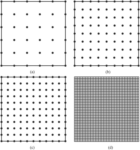
Table 2. The detailed boundary element models.

Model	Boundary elements	Boundary nodes	Internal nodes	Total nodes
(a)	20	20	16	36
(b)	32	32	49	81
(c)	40	40	81	121

The direct problem is solved with the time step $\mathrm{\Delta }\tau =0.01\mathrm{s}$. The temperature distribution at $\tau =0.5\mathrm{s}$ is shown in Figure 2. In cases (a), (b) and (c), the temperature distribution is solved by the DT-DRBEM. The results in case (d) are obtained by the finite element analysis software ANSYS 12.0.

Figure 2. The temperature distribution for different computational models. (a) BEM 1, (b) BEM 2, (c) BEM 3, (d) FEM.

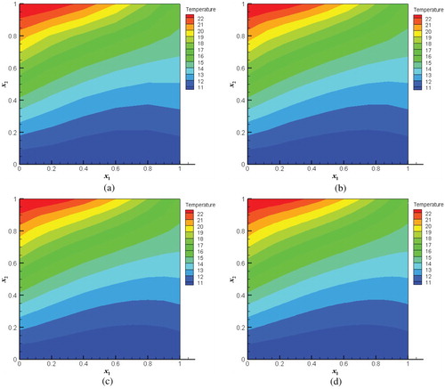
From Figure 2, it can be seen that the results by the proposed method are close to the finite element analysis. With reference to the results of case (d), the maximum relative errors in cases (a) (b) (c) are 0.843%, 0.653% and 0.573%, the root mean square deviations are 0.00455, 0.00228 and 0.00161, respectively. It can be noted that with the increase of boundary and internal nodes, the results are more accurate.

In addition, based on the model (c), the stability of the DT-DRBEM is also validated by comparing with the FD-DRBEM. The results for different time steps are summarized in Table 3.

Table 3. The comparison of DT-DRBEM and FD-DRBEM.

	DT-DRBEM			FD-DRBEM
Nodes	$\mathrm{\Delta }\tau =0.05$	$\mathrm{\Delta }\tau =0.01$	$\mathrm{\Delta }\tau =0.005$	$\mathrm{\Delta }\tau =0.05$	$\mathrm{\Delta }\tau =0.01$	$\mathrm{\Delta }\tau =0.005$
(0.2, 0.2)	11.590287	11.590287	11.590287	11.585383	11.590287	11.590287
(0.2, 0.6)	16.069455	16.069455	16.069455	16.066344	16.069454	16.069454
(0.4, 0.8)	17.726167	17.726167	17.726167	17.720308	17.726167	17.726167
(0.6, 0.4)	12.369837	12.369837	12.369837	12.370289	12.369837	12.369837
(0.8, 0.6)	13.699417	13.699417	13.699417	13.697171	13.699412	13.699412

From Table 3, it can be observed that the same results can be obtained when the different time steps are considered for the DT-DRBEM. But for the FD-DRBEM, the results have some changes for different time steps 0.05s, 0.01s and 0.005s. It implies that the proposed method is more stable than the FD-DRBEM. Therefore, the DT-DRBEM is an efficient and stable method to solve the transient heat conduction problem for orthotropic FGMs.

In order to compare the L-M algorithm and the CGM, the thermal conductivities are identified by taking the model (c) into consideration. The exact parameters $a_1=2.0,a_2=0.1,a_3=1.0,a_4=0.2$. Three different initial thermal conductivities are considered and the tolerance is $\epsilon ={10}^{-7}$. The results are computed by a FORTRAN compiler combined with the MATLAB software and the computations are running on a PC with Inter Core i5 and 4G RAM. The results are given in Table 4.

Table 4. The comparison of the L-M and the CGM.

	Estimated value		Iteration number		Computation time(s)
Initial value	L-M	CGM	L-M	CGM	L-M	CGM
$a_1=1.0$, $a_2=0.05$	$a_1=2.000$, $a_2=0.100$	$a_1=1.990$, $a_2=0.107$	7	79	50	8863
$a_3=0.5$, $a_4=0.1$	$a_3=1.000$, $a_4=0.200$	$a_3=0.995$, $a_4=0.206$
$a_1=1.0$, $a_2=1.0$	$a_1=2.000$, $a_2=0.100$	$a_1=1.998$, $a_2=0.100$	7	105	56	11232
$a_3=1.0$, $a_4=1.0$	$a_3=1.000$, $a_4=0.200$	$a_3=1.004$, $a_4=0.198$
$a_1=3.0$, $a_2=0.15$	$a_1=2.000$, $a_2=0.100$	$a_1=1.994$, $a_2=0.103$	6	154	41	17810
$a_3=1.5$, $a_4=0.3$	$a_3=1.000$, $a_4=0.200$	$a_3=1.002$, $a_4=0.200$

From Table 4, it can be seen that both methods can obtain the reliable results with different initial guesses. The L-M algorithm is more accurate than the CGM. The L-M algorithm spends fewer iterations and less computation time than the CGM. It indicates that the L-M algorithm is a more efficient and accurate method for inverse analysis relative to the CGM.

4.2. Example 2

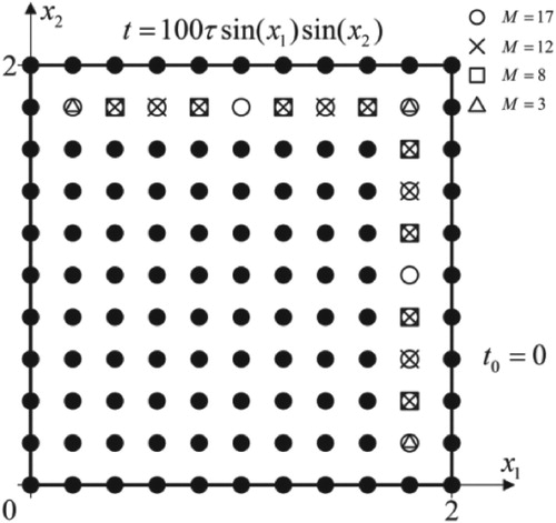
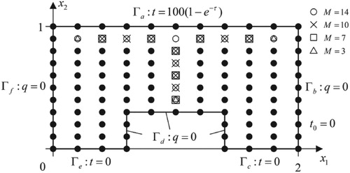
As shown in Figure 3, a square plate with side length 2 m is considered. The boundary is divided into 40 linear elements and 81 internal points are uniformly distributed in the domain. The boundary condition is $t=100\tau \sin \left(x_1\right)\sin \left(x_2\right)$ and the initial condition is $t_0=0$. The thermal conductivities ${\lambda }_{11}=a_1{e}^{a_2{x}_1}$, ${\lambda }_{22}=a_3{e}^{a_4{x}_2}$. The exact parameters $a_1=1.0$, $a_2=0.3$, $a_3=2.0$ and $a_4=0.2$.

Figure 3. DRBEM computational model.

4.2.1. Influence of initial guesses

The initial guesses are taken as 1/6, 1/3, 1.5 and 2 times of the exact parameters values. As shown in Figure 3, 17 measurement points are selected. Figure 4 shows the parameter convergence processes and the objective function versus iteration number. Table 5 lists the results for different initial guesses.

Figure 4. The results for different initial guesses. (a) ${\mathit{a}}_{\mathrm{i}\mathrm{n}\mathrm{i}}={\mathit{a}}_{\mathrm{e}\mathrm{x}\mathrm{a}}/6$, (b) ${\mathit{a}}_{\mathrm{i}\mathrm{n}\mathrm{i}}={\mathit{a}}_{\mathrm{e}\mathrm{x}\mathrm{a}}/3$, (c) ${\mathit{a}}_{\mathrm{i}\mathrm{n}\mathrm{i}}=1.5{\mathit{a}}_{\mathrm{e}\mathrm{x}\mathrm{a}}$, (d) ${\mathit{a}}_{\mathrm{i}\mathrm{n}\mathrm{i}}=2{\mathit{a}}_{\mathrm{e}\mathrm{x}\mathrm{a}}$_.

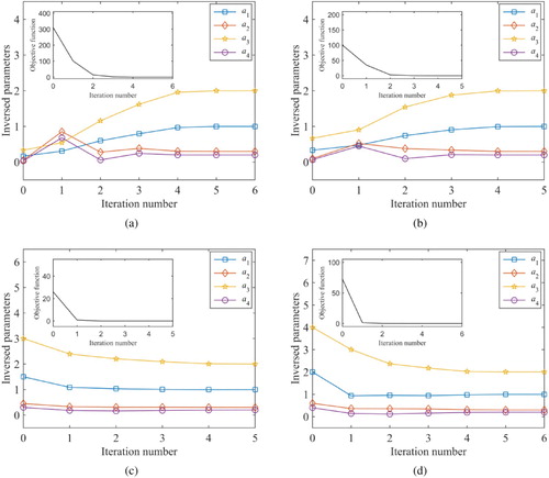
Table 5. The inverse results for different initial guesses.

		${\mathit{a}}_{\mathrm{i}\mathrm{n}\mathrm{i}}={\mathit{a}}_{\mathrm{e}\mathrm{x}\mathrm{a}}/6$	${\mathit{a}}_{\mathrm{i}\mathrm{n}\mathrm{i}}={\mathit{a}}_{\mathrm{e}\mathrm{x}\mathrm{a}}/3$	${\mathit{a}}_{\mathrm{i}\mathrm{n}\mathrm{i}}=1.5{\mathit{a}}_{\mathrm{e}\mathrm{x}\mathrm{a}}$	${\mathit{a}}_{\mathrm{i}\mathrm{n}\mathrm{i}}=2{\mathit{a}}_{\mathrm{e}\mathrm{x}\mathrm{a}}$
	${\mathit{a}}_{\mathrm{e}\mathrm{a}\mathrm{x}}$	${\mathit{a}}_{\mathrm{i}\mathrm{n}\mathrm{v}}$	${\mathit{a}}_{\mathrm{i}\mathrm{n}\mathrm{v}}$	${\mathit{a}}_{\mathrm{i}\mathrm{n}\mathrm{v}}$	${\mathit{a}}_{\mathrm{i}\mathrm{n}\mathrm{v}}$
$a_1$	1.000000	1.000000	0.999969	0.999913	1.000000
$a_2$	0.300000	0.300001	0.300004	0.300055	0.300000
$a_3$	2.000000	2.000000	1.999989	2.000141	2.000002
$a_4$	0.200000	0.200000	0.199998	0.199954	0.200000

As shown in Figure 4, it can be seen that all the cases can obtain good results. The maximum objective function value reduces from $3.10\times 10^2$ to $1.20\times 10^{-11}$ within 6 iterations. In addition, the number of iterations is not sensitive to the initial guesses. Table 5 shows that the inverse results are in good agreement with the exact solutions.

4.2.2. Influence of number of measurement points

In this section, the influence of number of measurement points is considered. The number of measurement points is taken as 3, 8, 12 and 17, respectively. The convergence processes are shown in Figure 5. The detailed results are listed in Table 6.

Figure 5. The results for different number of measurement points. (a) 3 measurement points, (b) 8 measurement points, (c) 12 measurement points, (d) 17 measurement points.

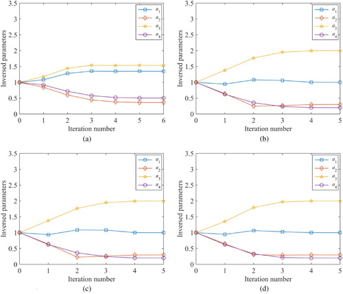
Table 6. The inverse results for different measurement points.

		$M=3$	$M=8$	$M=12$	$M=17$
	${\mathit{a}}_{\mathrm{e}\mathrm{a}\mathrm{x}}$	${\mathit{a}}_{\mathrm{i}\mathrm{n}\mathrm{v}}$	${\mathit{a}}_{\mathrm{i}\mathrm{n}\mathrm{v}}$	${\mathit{a}}_{\mathrm{i}\mathrm{n}\mathrm{v}}$	${\mathit{a}}_{\mathrm{i}\mathrm{n}\mathrm{v}}$
$a_1$	1.000000	1.349656	0.999995	1.000000	1.000001
$a_2$	0.300000	0.363770	0.300001	0.299998	0.299999
$a_3$	2.000000	1.535150	1.999987	1.999968	2.000000
$a_4$	0.200000	0.504574	0.200006	0.200015	0.200000

Figure 5 shows that all the results can achieve convergence. It is observed that the number of measurement points has great influence on the inverse results. From Table 6, it can be seen that the inverse analysis can’t recover the exact thermal properties when the number of measurement points is 3. However, the inverse results can be estimated precisely when the number is more than 8.

4.2.3. Influence of measurement errors

The measurement errors 1%, 3%, and 5% are considered. 17 measurement points are chosen for the inverse predictions. The results are summarized in Table 7.

Table 7. The inverse results for different measurement errors.

		$\sigma =1\mathrm{\%}$		$\sigma =3\mathrm{\%}$		$\sigma =5\mathrm{\%}$
	${\mathit{a}}_{\mathrm{e}\mathrm{a}\mathrm{x}}$	${\mathit{a}}_{\mathrm{i}\mathrm{n}\mathrm{v}}$	$E_{\mathrm{r}\mathrm{e}\mathrm{l}}$	${\mathit{a}}_{\mathrm{i}\mathrm{n}\mathrm{v}}$	$E_{\mathrm{r}\mathrm{e}\mathrm{l}}$	${\mathit{a}}_{\mathrm{i}\mathrm{n}\mathrm{v}}$	$E_{\mathrm{r}\mathrm{e}\mathrm{l}}$
$a_1$	1.000000	1.012957	1.30%	0.965499	3.45%	0.952461	4.75%
$a_2$	0.300000	0.290590	3.14%	0.310721	3.57%	0.312060	4.02%
$a_3$	2.000000	1.981359	0.93%	1.926160	3.69%	1.908671	4.57%
$a_4$	0.200000	0.205280	2.64%	0.208039	4.02%	0.215146	7.57%

From Table 7, it can be seen that the measurement errors have great influence on the inverse results. As expected, the inversion accuracy decreases when the measurement error increases.

4.3. Example 3

In this example, as shown in Figure 6, the mixed boundary value problem is considered in a polygonal plate. The boundary is divided into 46 linear elements and 66 internal collocation points are uniformly distributed in the domain. The initial condition is $t_0=0$. The top and bottom of the plate are maintained at temperature $t=100(1-e^{-\tau })$ and $t=0$, respectively. The remaining five edges are insulated. The thermal conductivities ${\lambda }_{11}=a_1+a_2{x}_1$, ${\lambda }_{22}=a_3+a_4{x}_2+a_5{x}_2^2$. The exact parameters $a_1=2.0$, $a_2=0.5$, $a_3=1.0$, $a_4=0.4$ and $a_5=0.2$.

Figure 6. DRBEM computational model.

4.3.1. Influence of initial guesses

The initial guesses are taken as 1/6, 1/3, 1.5 and 2 times of the exact parameters. As shown in Figure 6, the measurement points are taken as 14. The convergence processes for each inversed parameter and the decrease of objective function versus the iteration number are exhibited in Figure 7. Table 8 lists the results for different initial guesses.

Figure 7. The results for different initial guesses. (a) ${\mathit{a}}_{\mathrm{i}\mathrm{n}\mathrm{i}}={\mathit{a}}_{\mathrm{e}\mathrm{x}\mathrm{a}}/6$, (b) ${\mathit{a}}_{\mathrm{i}\mathrm{n}\mathrm{i}}={\mathit{a}}_{\mathrm{e}\mathrm{x}\mathrm{a}}/3$, (c) ${\mathit{a}}_{\mathrm{i}\mathrm{n}\mathrm{i}}=1.5{\mathit{a}}_{\mathrm{e}\mathrm{x}\mathrm{a}}$, (d) ${\mathit{a}}_{\mathrm{i}\mathrm{n}\mathrm{i}}=2{\mathit{a}}_{\mathrm{e}\mathrm{x}\mathrm{a}}$_.

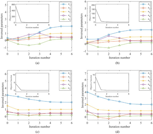
Table 8. The inverse results for different initial guesses.

		${\mathit{a}}_{\mathrm{i}\mathrm{n}\mathrm{i}}={\mathit{a}}_{\mathrm{e}\mathrm{x}\mathrm{a}}/6$	${\mathit{a}}_{\mathrm{i}\mathrm{n}\mathrm{i}}={\mathit{a}}_{\mathrm{e}\mathrm{x}\mathrm{a}}/3$	${\mathit{a}}_{\mathrm{i}\mathrm{n}\mathrm{i}}=1.5{\mathit{a}}_{\mathrm{e}\mathrm{x}\mathrm{a}}$	${\mathit{a}}_{\mathrm{i}\mathrm{n}\mathrm{i}}=2{\mathit{a}}_{\mathrm{e}\mathrm{x}\mathrm{a}}$
	${\mathit{a}}_{\mathrm{e}\mathrm{a}\mathrm{x}}$	${\mathit{a}}_{\mathrm{i}\mathrm{n}\mathrm{v}}$	${\mathit{a}}_{\mathrm{i}\mathrm{n}\mathrm{v}}$	${\mathit{a}}_{\mathrm{i}\mathrm{n}\mathrm{v}}$	${\mathit{a}}_{\mathrm{i}\mathrm{n}\mathrm{v}}$
$a_1$	2.000000	1.999925	2.000002	2.000349	2.000536
$a_2$	0.500000	0.499965	0.499998	0.500031	0.500087
$a_3$	1.000000	1.000024	1.000000	0.999942	0.999908
$a_4$	0.400000	0.399968	0.400001	0.400367	0.400720
$a_5$	0.200000	0.200026	0.200000	0.199715	0.199373

From Figure 7, it can be observed that the accurate results can be obtained when different initial guesses are used. The maximum objective function value decreases from $5.41\times 10^2$ to $3.66\times 10^{-8}$. The number of iterations is also not sensitive to the initial guesses. Table 8 shows that the results keep good agreement with the exact values.

4.3.2. Influence of number of measurement points

As shown in Figure 6, the number of measurement points is taken as 3, 7, 10 and 14, respectively. The corresponding convergence processes are shown in Figure 8 and the results are listed in Table 9.

Figure 8. The results for different number of measurement points. (a) 3 measurement points, (b) 7 measurement points, (c) 10 measurement points, (d) 14 measurement points.

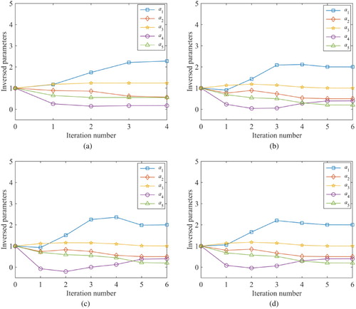
Table 9. The inverse results for different number of measurement points.

		$M=3$	$M=7$	$M=10$	$M=14$
	${\mathit{a}}_{\mathrm{e}\mathrm{a}\mathrm{x}}$	${\mathit{a}}_{\mathrm{i}\mathrm{n}\mathrm{v}}$	${\mathit{a}}_{\mathrm{i}\mathrm{n}\mathrm{v}}$	${\mathit{a}}_{\mathrm{i}\mathrm{n}\mathrm{v}}$	${\mathit{a}}_{\mathrm{i}\mathrm{n}\mathrm{v}}$
$a_1$	2.000000	2.272941	2.000054	2.000293	2.000020
$a_2$	0.500000	0.569939	0.500029	0.499945	0.500004
$a_3$	1.000000	1.240204	1.000027	1.000066	1.000006
$a_4$	0.400000	0.184487	0.399926	0.399976	0.399990
$a_5$	0.200000	0.552493	0.200051	0.200085	0.200013

Figure 8 shows that the results can achieve convergence for different measurement point number. From Table 9, it can be seen that the results are not good with 3 measurement points, but accurate results are obtained when the number of measurement points increases to 7.

4.3.3. Influence of measurement errors

The measurement errors are taken as 1%, 3%, and 5%. As shown in Figure 6, 14 measurement points are selected. The results are summarized in Table 10.

Table 10. The inverse results for different measurement errors.

		$\sigma =1\mathrm{\%}$		$\sigma =3\mathrm{\%}$		$\sigma =5\mathrm{\%}$
	${\mathit{a}}_{\mathrm{e}\mathrm{a}\mathrm{x}}$	${\mathit{a}}_{\mathrm{i}\mathrm{n}\mathrm{v}}$	$E_{\mathrm{r}\mathrm{e}\mathrm{l}}$	${\mathit{a}}_{\mathrm{i}\mathrm{n}\mathrm{v}}$	$E_{\mathrm{r}\mathrm{e}\mathrm{l}}$	${\mathit{a}}_{\mathrm{i}\mathrm{n}\mathrm{v}}$	$E_{\mathrm{r}\mathrm{e}\mathrm{l}}$
$a_1$	2.000000	1.959837	2.01%	2.076655	3.83%	2.062476	3.12%
$a_2$	0.500000	0.504104	0.82%	0.471220	5.76%	0.455133	8.97%
$a_3$	1.000000	1.010316	1.03%	1.004463	0.45%	1.028090	2.81%
$a_4$	0.400000	0.384563	3.86%	0.390555	2.36%	0.395801	1.05%
$a_5$	0.200000	0.207147	3.57%	0.218355	9.18%	0.245349	22.7%

From Table 10, for $a_1$, $a_3$ and $a_4$, their error does not increase monotonously as the measurement error increase. It is because the thermal conductivity is related to all the parameters rather than one or two parameters alone. Substituting all parameters into the function expression of thermal conductivity, it can be found that the inversion accuracy decreases as expected as the measurement error increases. In addition, the relative error of parameter $a_5$ is bigger than $a_3$ and $a_4$. The reason for this is that the $a_5$ is the smallest among the three parameters and its relative error looks large.

5. Conclusion

In this paper, the thermal conductivity of orthotropic FGMs for transient heat conduction problems is identified by the DT-DRBEM coupled with L-M algorithm. The DTM is used as an efficient and accurate time-domain processing method. The DRBEM is applied to transform the domain integral into the boundary integral. In addition, the L-M algorithm is an excellent optimization algorithm to minimize the objective function and recover the desired thermal properties. The influence of different initial values, number of measurement points and measurement errors on the inverse results are investigated. Some conclusions can be drawn:

1. The DRBEM combined with the DTM is an efficient way to solve the transient heat conduction problem for orthotropic FGMs. And the DTM is more stable than the FDM.

2. The L-M algorithm is a more efficient and accurate method for inverse analysis relative to the CGM.

3. The results show that the method can obtain reliable inverse results by selecting the appropriate initial guesses.

4. The number of measurement points has effect on the inverse results. To guarantee the accuracy of inversed results, enough measurement points are needed.

5. The measurement errors also have a great influence on the inverse results. The less the measurement errors are, the more accurate the inverse results are.

Disclosure statement

No potential conflict of interest was reported by the authors.

ORCID

Huan-Lin Zhou http://orcid.org/0000-0003-3678-7688

Additional information

Funding

The research is supported by the National Natural Science Foundation of China [11672098].

References

- Suresh S, Mortensen A. Fundamentals of functionally graded materials. London: IOM Communications; 1998.
- Lee WY, Stinton DP, Berndt CC, et al. Concept of functionally graded materials for advanced thermal barrier coating applications. J Am Ceram Soc. 1996;79(12):3003–3012.
- Miyamoto Y, Kaysser WA, Rabin BH, et al. Functionally graded materials: design, processing and applications. Dordrecht: Kluwer Academic Publishers; 1999.
- Jha DK, Kant T, Singh RK. A critical review of recent research on functionally graded plates. Compos Struct. 2013;96(4):833–849.
- Gupta A, Talha M. Recent development in modeling and analysis of functionally graded materials and structures. Prog Aerosp Sci. 2015;79:1–14.
- Flach GP, Özişik MN. Inverse heat conduction problem of simultaneously estimating spatially varying thermal conductivity and heat capacity per unit volume. Numer Heat Transf. 1989;16(2):249–266.
- Zajas J, Heiselberg P. Determination of the local thermal conductivity of functionally graded materials by a laser flash method. Int J Heat Mass Transf. 2013;60:542–548.
- Chen B, Chen W, Wei X. Characterization of space-dependent thermal conductivity for nonlinear functionally graded materials. Int J Heat Mass Transf. 2015;84:691–699.
- Nedin R, Nesterov S, Vatulyan A. Identification of thermal conductivity coefficient and volumetric heat capacity of functionally graded materials. Int J Heat Mass Transf. 2016;102:213–218.
- Naveira-Cotta CP, Orlande HRB, Cotta RM. Combining integral transforms and Bayesian inference in the simultaneous identification of variable thermal conductivity and thermal capacity in heterogeneous media. ASME J Heat Transf. 2011;133(11):1301–1311.
- Chen WL, Chou HM, Yang YC. An inverse problem in estimating the space-dependent thermal conductivity of a functionally graded hollow cylinder. Compos Part B. 2013;50:112–119.
- Brebbia CA. The boundary element method for engineers. London: Pentech Press; 1980.
- Cheng AHD, Cheng DT. Heritage and early history of the boundary element method. Eng Anal Bound Elem. 2005;29(3):268–302.
- Partridge PW, Brebbia CA, Wrobel LC. Dual reciprocity boundary element method. Southampton: Computational Mechanics Publications; 1992.
- Tanaka M, Matsumoto T, Takakuwa S. Dual reciprocity BEM for time-stepping approach to the transient heat conduction problem in nonlinear materials. Comput Methods Appl Mech Eng. 2006;195(37–40):4953–4961.
- Ishiguro S, Tanaka M. Analysis of two-dimensional nonlinear transient heat conduction in anisotropic solids by boundary element method using dual reciprocity method. J Environ Eng. 2007;2(2):266–277.
- Sutradhar A, Paulino GH, Gray LJ. Transient heat conduction in homogeneous and non-homogeneous materials by the Laplace transform Galerkin boundary element method. Eng Anal Bound Elem. 2002;26(2):119–132.
- Sladek J, Sladek V, Atluri SN. Meshless local Petrov-Galerkin method for heat conduction problem in an anisotropic medium. CMES Comput Model Eng Sci. 2004;6(3):309–318.
- Sladek J, Sladek V, Hellmich C, et al. Heat conduction analysis of 3-D axisymmetric and anisotropic FGM bodies by meshless local Petrov-Galerkin method. Comput Mech. 2007;39(3):323–333.
- Wang H, Qin QH, Kang YL. A meshless model for transient heat conduction in functionally graded materials. Comput Mech. 2006;38(1):51–60.
- Li G, Guo S, Zhang J, et al. Transient heat conduction analysis of functionally graded materials by a multiple reciprocity boundary face method. Eng Anal Bound Elem. 2015;60:81–88.
- Zhou JK. Differential transformation and its applications for electrical circuits. Wuhan: Huazhong University Press; 1986.
- Yaghoobi H, Torabi M. The application of differential transformation method to nonlinear equations arising in heat transfer. Int Commun Heat Mass. 2011;38(6):815–820.
- Hassan IHAH. Differential transformation technique for solving higher-order initial value problems. Appl Math Comput. 2004;154(2):299–311.
- Jang MJ, Yeh YL, Chen CL, et al. Differential transformation approach to thermal conductive problems with discontinuous boundary condition. Appl Math Comput. 2010;216(8):2339–2350.
- Moradi A, Hayat T, Alsaedi A. Convection-radiation thermal analysis of triangular porous fins with temperature-dependent thermal conductivity by DTM. Energy Convers Manage. 2014;77:70–77.
- Chu HP, Lo CY. Application of the hybrid differential transform-finite difference method to nonlinear transient heat conduction problems. Numer Heat Transf Part A. 2007;53(3):295–307.
- Alifanov OM, Nenarokomov AV, Budnik SA, et al. Identification of thermal properties of materials with applications for spacecraft structures. Inverse Probl Sci Eng. 2004;12(5):579–594.
- Huang CH, Huang CY. An inverse problem in estimating simultaneously the effective thermal conductivity and volumetric heat capacity of biological tissue. Appl Math Model. 2007;31(9):1785–1797.
- Alifanov OM, Budnik SA, Nenarokomov AV, et al. Estimation of thermal properties of materials with application for inflatable spacecraft structure testing. Inverse Probl Sci Eng. 2012;20(5):677–690.
- Greiby I, Mishra DK, Dolan KD. Inverse method to sequentially estimate temperature-dependent thermal conductivity of cherry pomace during nonisothermal heating. J Food Eng. 2014;127:16–23.
- Fedchenia II, van Hassel BA, Brown R. Solution of inverse thermal problem for assessment of thermal parameters of engineered H2 storage materials. Inverse Probl Sci Eng. 2015;23(3):425–442.
- Hafid M, Lacroix M. An inverse heat transfer method for predicting the thermal characteristics of a molten material reactor. Appl Therm Eng. 2016;108:140–149.
- Huang CH, Chin SC. A two-dimensional inverse problem in imaging the thermal conductivity of a non-homogeneous medium. Int J Heat Mass Transf. 2000;43(22):4061–4071.
- Mera NS, Elliott L, Ingham DB, et al. An iterative bem for the Cauchy steady state heat conduction problem in an anisotropic medium with unknown thermal conductivity tensor. Inverse Probl Sci Eng. 2000;8(6):579–607.
- Mera NS, Elliott L, Ingham DB, et al. Use of the boundary element method to determine the thermal conductivity tensor of an anisotropic medium. Int J Heat Mass Transf. 2001;44(21):4157–4167.
- Ardakani MD, Khodadad M. Identification of thermal conductivity and the shape of an inclusion using the boundary elements method and the particle swarm optimization algorithm. Inverse Probl Sci Eng. 2009;17(7):855–870.
- Imani A, Ranjbar AA, Esmkhani M. Simultaneous estimation of temperature-dependent thermal conductivity and heat capacity based on modified genetic algorithm. Inverse Probl Sci Eng. 2006;14(7):767–783.
- Hematiyan MR, Khosravifard A, Shiah YC. A novel inverse method for identification of 3D thermal conductivity coefficients of anisotropic media by the boundary element analysis. Int J Heat Mass Transf. 2015;89:685–693.
- Kim SK, Jung BS, Kim HJ, et al. Inverse estimation of thermophysical properties for anisotropic composite. Exp Therm Fluid Sci. 2003;27(6):697–704.
- Mohebbi F, Sellier M, Rabczuk T. Estimation of linearly temperature-dependent thermal conductivity using an inverse analysis. Int J Therm Sci. 2017;117:68–76.
- Mohebbi F, Sellier M. Identification of space-and temperature-dependent heat transfer coefficient. Int J Therm Sci. 2018;128:28–37.
- Dulikravich GS, Reddy SR, Pasqualette MA, et al. Inverse determination of spatially varying material coefficients in solid objects. J Inverse Ill-Pose Prob. 2016;24(2):181–194.
- Reddy SR, Dulikravich GS, Zeidi SMJ. Non-destructive estimation of spatially varying thermal conductivity in 3D objects using boundary thermal measurements. Int J Therm Sci. 2017;18:488–496.
- Reddy SR, Dulikravich GS, Zeidi SMJ. Inverse determination of spatially varying heat capacity and thermal conductivity in arbitrary 2D objects. Danbury: ICMHT Digital Library; 2017.
- Marquardt DW. An algorithm for least-squares estimation of nonlinear parameters. J Soc Ind Appl Math. 1963;11(2):431–441.
- Fletcher R, Powell MJD. A rapidly convergent descent method for minimization. Comput J. 1963;6(2):163–168.
- Wright S, Nocedal J. Numerical optimization. New York (NY): Springer Science; 1999.
- Sawaf B, Ozisik MN, Jarny Y. An inverse analysis to estimate linearly temperature dependent thermal conductivity components and heat capacity of an orthotropic medium. Int J Heat Mass Transf. 1995;38(16):3005–3010.
- Rodriguez-Quinonez JC, Sergiyenko O, Gonzalez-Navarro FF, et al. Surface recognition improvement in 3D medical laser scanner using Levenberg-Marquardt method. Signal Process. 2013;93(2):378–386.
- Cui M, Gao XW, Zhang JB. A new approach for the estimation of temperature-dependent thermal properties by solving transient inverse heat conduction problems. Int J Therm Sci. 2012;58:113–119.
- Cui M, Zhao Y, Xu BB, et al. Inverse analysis for simultaneously estimating multi-parameters of temperature-dependent thermal conductivities of an Inconel in a reusable metallic thermal protection system. Appl Therm Eng. 2017;125:480–488.