Identification of distributed dynamic excitation based on Taylor polynomial iteration and cubic Catmull–Rom spline interpolation

ABSTRACT

This paper devotes to identifying the distributed dynamic excitation in time domain via a comprehensive algorithm combining Taylor polynomial iteration and cubic Catmull–Rom spline interpolation. Under the premise of obtaining structural characteristic and node response, Taylor polynomial iteration algorithm is introduced to reconstruct the distributed force amplitudes in node positions of a simple supported beam. Then the load amplitudes at nodes are used as control points, thereby cubic Catmull–Rom spline is adopted to interpolate the complete spatial course of distributed dynamic load along the whole beam. Numerical examples illustrate that the integration method is able to acquire relatively accurate identification result of distributed force. Furthermore, noise immunity of this method is investigated and it displays a strong anti-noise performance.

KEYWORDS:

• Distributed dynamic excitation
• time domain
• Taylor polynomial iteration
• cubic Catmull–Rom spline interpolation
• noise immunity

AMS SUBJECT CLASSIFICATIONS:

• 74M20
• 34K29

1. Introduction

There are a lot of vibration phenomena in engineering practices. So the research area of structural dynamics is built up to deal with vibration problems. Identification of dynamic excitation is a crucial branch in structural dynamics. The core thought of load identification is to take dynamic response and system characteristic as known conditions and calculate the force time history through specific algorithm. Force identification result is conducive to health monitoring, failure diagnosis and dependability analysis of the vibration system. Along with the rapid development of engineering technology nowadays, force identification is exerting a greater influence for engineering vibration.

In the past decades, researchers have implemented large numbers of studies in the field of load identification. In particular, concentrated load identification is more mature. Authors in [1–3] reconstructed the amplitude of concentrated load in frequency domain. And in [4–8], the authors provided different algorithms to compute the concentrated force time history in time domain as well. Apart from frequency domain and time domain methods, some intelligent algorithms [9,10] emerged as well. Meanwhile, Liu et al. proposed interval analysis method [11] and Gegenbauer polynomial expansion theory [12] separately to determine the bounds of concentrated load aiming at uncertain structure. Moreover, regularization technique is commonly employed to deal with the ill-posedness problem in force identification. For example, an efficient interpolation-based method is proposed to reduce ill-posedness availably and identify dynamic load stably in [13]. Authors in [14–16] adopted optimal Tikhonov regularization to produce reasonable solutions. In recent studies, sparse regularization was applied in [17–19] and reached higher accuracy than Tikhonov regularization.

There are relatively fewer researches on the identification of distributed load. The authors in [20] developed an improved method which defines the basis functions over the finite region of the force and reconstructed distributed forces. Djamaa et al. [21] used the finite-difference method to identify the position of distributed force which excites a cylindrical shell from its internal side. Jiang and Hu [22] presented a new approach based on a mode-selection method and an idea of consistent spatial expression to reconstruct the distributed dynamic loads on an Euler beam from the beam response. In [23], the authors put forward a convenient and efficient approach to rebuild two-dimensional distributed excitations on a damped thin elastic plate from its steady-state dynamic response. In [24], a new approach based on shape function method of moving least square fitting (SFM_MLSF) and polynomial selection technique was proposed for distributed dynamic load identification. Li et al. [25] presented an inverse approach based on Green's function method and orthogonal polynomial to reconstruct distributed load. Lourens and Fallais [26] used Kalman-type filters to estimate the full-field dynamic response and identified a set of response-driving equivalent forces from the measurements. As a typical distributed load, wind load was inversely reconstructed [27] in time domain with an augmented impulse response matrix.

However, existing research methods for distributed excitation identification still have some limitations. On one hand, these methods are mainly carried out under modal coordinates. Matrix of modal shape is essential and physical parameters need to be transformed into modal parameters by modal transformation. On the other hand, these methods can only identify the load amplitudes in specified positions of measured response points rather than the whole beam. There are lots of blank areas among nodes. For these blank areas, distributed force also exists. In current studies, researchers usually neglect these blank areas and connect the node amplitudes directly. So it can’t reflect the true situation of distributed excitation.

In order to overcome above drawbacks, this paper sets up a comprehensive method which integrates Taylor polynomial iteration and cubic Catmull–Rom spline interpolation to identify distributed dynamic load in time domain.

Taylor polynomial iteration [28,29] is a step-by-step integration algorithm with high accuracy in essence. It expresses dynamic response vector as Taylor polynomial first. After a series of formula deduction, an explicit discrete equation which combines input force, output response and structural characteristic together is achieved in the end. This algorithm was originally proposed for centralized load identification and it is pulled into distributed excitation identification area for the first time in this paper.

As an interpolation method, cubic Catmull–Rom spline [30,31] was often used in engineering applications because it is able to automatically interpolate the given control points. And this paper creatively utilizes cubic Catmull–Rom spline to interpolate the distributed load on the whole beam.

Generally speaking, proposed method is operated in two steps. In the first step, one calculates distributed force’s time histories at measured response points with Taylor polynomial iteration algorithm. In the second step, cubic Catmull–Rom spline interpolation is applied to reconstruct the distributed dynamic loads of the whole beam on the basis of former step. The load values obtained by first step are control points needed in second step.

2. Taylor polynomial iteration algorithm for distributed load identification

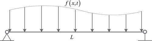
A simple supported beam under distributed excitation $f\left(x,t\right)$ is established in Figure 1. Supposing the number of node response sensors is m, then the beam is evenly divided into m segments. The centres of segments are set to be beam nodes and the sensors are distributed at these nodes. The number of degrees of freedom is $d=2\left(m+2\right)$. The structural dynamics equation can be written as (1) $\mathit{M}\ddot{\mathit{X}}\left(t\right)+\mathit{C}\dot{\mathit{X}}\left(t\right)+\mathit{K}X\left(t\right)=\mathit{F}\left(t\right),$(1) where $\mathit{M}$, $\mathit{C}$ and $\mathit{K}$ are mass, damping and stiffness matrices. $\ddot{\mathit{X}}\left(t\right)$, $\dot{\mathit{X}}\left(t\right)$, $\mathit{X}\left(t\right)$ denote acceleration, velocity and displacement responses. $\mathit{F}\left(t\right)$ is the load vector in all degrees of freedom. In this research, one needs to identify particular forces in m sensor locations. These forces are expressed by approximating distributed force as concentrated force $F_{\kappa }\left(t\right)$, namely (2) $F_{\kappa }\left(t\right)={\int }_{L_{\kappa }}f\left(x,t\right)\text{d}x,\kappa =1-m.$(2)

Figure 1. Simple supported beam subjected to distributed excitation.

Equation (1) is a two-order coupled differential equation. In order to solve this equation, the whole time history is discretized into many small time periods. For each time period $\left[t,t+\mathrm{\Delta }t\right]$, one devotes to finding a fixed relationship between $\ddot{\mathit{X}}\left(t\right)$, $\dot{\mathit{X}}\left(t\right)$, $\mathit{X}\left(t\right)$ and $\ddot{\mathit{X}}\left(t+\mathrm{\Delta }t\right)$, $\dot{\mathit{X}}\left(t+\mathrm{\Delta }t\right)$, $\mathit{X}\left(t+\mathrm{\Delta }t\right)$. Once the relationship is determined, start the loop computation from time 0 and the dynamic response at each time point can be obtained. Therefore, to achieve the step-by-step calculation, one must make an assumption for the relationship of dynamic responses between adjacent time points. Here Taylor polynomial is an appropriate choice to approximately express the fixed relationship mentioned above.

Response vectors are expanded into two-order Taylor polynomial in the neighbourhood of time $t$, namely: (3) $\ddot{\mathit{X}}\left(t+\tau \right)=\ddot{\mathit{X}}\left(t\right)+\tau {\mathit{\chi }}_1+\frac{{\tau }^2}{2}{\mathit{\chi }}_2,$(3) (4) $\dot{\mathit{X}}\left(t+\tau \right)=\dot{\mathit{X}}\left(t\right)+{\int }_0^{\tau }\ddot{\mathit{X}}\left(t+\tau \right)\text{d}\tau =\dot{\mathit{X}}\left(t\right)+\tau \ddot{\mathit{X}}\left(t\right)+\frac{{\tau }^2}{2}{\mathit{\chi }}_1+\frac{{\tau }^3}{6}{\mathit{\chi }}_2,$(4) (5) $\mathit{X}\left(t+\tau \right)=\mathit{X}\left(t\right)+{\int }_0^{\tau }\dot{\mathit{X}}\left(t+\tau \right)\text{d}\tau =\mathit{X}\left(t\right)+\tau \dot{\mathit{X}}\left(t\right)+\frac{{\tau }^2}{2}\ddot{\mathit{X}}\left(t\right)+\frac{{\tau }^3}{6}{\mathit{\chi }}_1+\frac{{\tau }^4}{24}{\mathit{\chi }}_2.$(5)

Next if the values of ${\mathit{\chi }}_1$ and ${\mathit{\chi }}_2$ are calculated, the iterative relationship of responses between neighbouring time points can be confirmed.

Substituting Equations (3), (4), (5) into Equation (1), one obtains: (6) ${\mathit{P}}_1\left(\tau \right){\mathit{\chi }}_1+{\mathit{P}}_2\left(\tau \right){\mathit{\chi }}_2=\mathit{Q}\left(\tau \right),$(6) where (7) ${\mathit{P}}_1\left(\tau \right)=\tau \mathit{M}+\frac{{\tau }^2}{2}\mathit{C}+\frac{{\tau }^3}{6}\mathit{K},$(7) (8) ${\mathit{P}}_2\left(\tau \right)=\frac{{\tau }^2}{2}\mathit{M}+\frac{{\tau }^3}{6}\mathit{C}+\frac{{\tau }^4}{24}\mathit{K},$(8) (9) $\mathit{Q}\left(\tau \right)=\mathit{F}\left(t+\tau \right)-\left(\mathit{M}+\tau \mathit{C}+\frac{{\tau }^2}{2}\mathit{K}\right)\ddot{\mathit{X}}\left(t\right)-\left(\mathit{C}+\tau \mathit{K}\right)\dot{\mathit{X}}\left(t\right)-\mathit{K}X\left(t\right).$(9)

Suppose the time interval of between two adjacent time points is $\Delta t$. As $\tau =\Delta t$, let ${\mathit{P}}_{11}={\mathit{P}}_1\left(\mathrm{\Delta }t\right)$, ${\mathit{P}}_{12}={\mathit{P}}_2\left(\mathrm{\Delta }t\right)$, ${\mathit{Q}}_1=\mathit{Q}\left(\mathrm{\Delta }t\right)$. As $\tau =1.1\Delta t$, let ${\mathit{P}}_{21}={\mathit{P}}_1\left(1.1\mathrm{\Delta }t\right)$, ${\mathit{P}}_{22}={\mathit{P}}_2\left(1.1\mathrm{\Delta }t\right)$, ${\mathit{Q}}_2=\mathit{Q}\left(1.1\mathrm{\Delta }t\right)$. After that one gets (10) $\left[\begin{array}{cc}{\mathit{P}}_{11}& {\mathit{P}}_{12}\\ {\mathit{P}}_{21}& {\mathit{P}}_{22}\end{array}\right]\left[\begin{array}{c}{\mathit{\chi }}_1\\ {\mathit{\chi }}_2\end{array}\right]=\left[\begin{array}{c}{\mathit{Q}}_1\\ {\mathit{Q}}_2\end{array}\right].$(10) Then ${\mathit{\chi }}_1$ and ${\mathit{\chi }}_2$ are computed as (11) $\left[\begin{array}{c}{\mathit{\chi }}_1\\ {\mathit{\chi }}_2\end{array}\right]={\left[\begin{array}{cc}{\mathit{P}}_{11}& {\mathit{P}}_{12}\\ {\mathit{P}}_{21}& {\mathit{P}}_{22}\end{array}\right]}^{-1}\left[\begin{array}{c}{\mathit{Q}}_1\\ {\mathit{Q}}_2\end{array}\right].$(11)

In Equation (11), ${\mathit{\chi }}_1$ and ${\mathit{\chi }}_2$ are both linear combinations of $\mathit{X}\left(t\right)$, $\dot{\mathit{X}}\left(t\right)$, $\ddot{\mathit{X}}\left(t\right)$, $\mathit{F}\left(t+\mathrm{\Delta }t\right)$ and $\mathit{F}\left(t+2\mathrm{\Delta }t\right)$. Once ${\mathit{\chi }}_1$ and ${\mathit{\chi }}_2$ are confirmed, the linear relationship of responses between neighbouring time points can be acquired. Suppose the time history totally samples n points and time $t_i$ is the $i$th time point, then (12) $\ddot{\mathit{X}}\left(t_i\right)={\ddot{\mathit{X}}}_i\dot{\mathit{X}}\left(t_i\right)={\dot{\mathit{X}}}_i\mathit{X}\left(t_i\right)={\mathit{X}}_i\mathit{F}\left(t_i\right)={\mathit{F}}_i.$(12) Bringing ${\mathit{\chi }}_1$ and ${\mathit{\chi }}_2$ back to Equations (3), (4) and (5), one gets the relationship of vibration responses in adjacent time points. After simplification, the equations are written as (13) ${\mathit{X}}_{i+1}={\mathit{A}}_1{\mathit{F}}_{i+1}+{\mathit{A}}_2{\mathit{F}}_{i+2}+{\mathit{A}}_d{\mathit{X}}_i+{\mathit{A}}_v{\dot{\mathit{X}}}_i+{\mathit{A}}_a{\ddot{\mathit{X}}}_i,$(13) (14) ${\dot{\mathit{X}}}_{i+1}={\mathit{B}}_1{\mathit{F}}_{i+1}+{\mathit{B}}_2{\mathit{F}}_{i+2}+{\mathit{B}}_d{\mathit{X}}_i+{\mathit{B}}_v{\dot{\mathit{X}}}_i+{\mathit{B}}_a{\ddot{\mathit{X}}}_i,$(14) (15) ${\ddot{\mathit{X}}}_{i+1}={\mathit{C}}_1{\mathit{F}}_{i+1}+{\mathit{C}}_2{\mathit{F}}_{i+2}+{\mathit{C}}_d{\mathit{X}}_i+{\mathit{C}}_v{\dot{\mathit{X}}}_i+{\mathit{C}}_a{\ddot{\mathit{X}}}_i.$(15)

A₁, A₂, A_d, A_v, A_a, B₁, B₂, B_d, B_v, B_a, C₁, C₂, C_d, C_v, C_a are all constant matrices with $d\times d$ dimensions. Combining Equations (13), (14) and (15) to obtain (16) ${\mathit{Y}}_i=\left[\begin{array}{c}{\mathit{X}}_{i+1}\\ {\dot{\mathit{X}}}_{i+1}\\ {\ddot{\mathit{X}}}_{i+1}\end{array}\right]=\left[\begin{array}{cc}{\mathit{A}}_1& {\mathit{A}}_2\\ {\mathit{B}}_1& {\mathit{B}}_2\\ {\mathit{C}}_1& {\mathit{C}}_2\end{array}\right]\left[\begin{array}{c}{\mathit{F}}_{i+1}\\ {\mathit{F}}_{i+2}\end{array}\right]+\left[\begin{array}{ccc}{\mathit{A}}_d& {\mathit{A}}_v& {\mathit{A}}_a\\ {\mathit{B}}_d& {\mathit{B}}_v& {\mathit{B}}_a\\ {\mathit{C}}_d& {\mathit{C}}_v& {\mathit{C}}_a\end{array}\right]\left[\begin{array}{c}{\mathit{X}}_i\\ {\dot{\mathit{X}}}_i\\ {\ddot{\mathit{X}}}_i\end{array}\right].$(16) Zero initial response is assumed. Through iterative processing, the response at time $t_i$ can be expressed as (17) ${\mathit{Y}}_i=\sum _{j=0}^{i-1}\left[\begin{array}{cc}{Z}_j& W_j\end{array}\right]\left[\begin{array}{c}{\mathit{F}}_{i-j}\\ {\mathit{F}}_{i-j+1}\end{array}\right],$(17) where (18) $\begin{array}{rl}& {\mathit{Z}}_j={\left[\begin{array}{ccc}{\mathit{A}}_d& {\mathit{A}}_v& {\mathit{A}}_a\\ {\mathit{B}}_d& {\mathit{B}}_v& {\mathit{B}}_a\\ {\mathit{C}}_d& {\mathit{C}}_v& {\mathit{C}}_a\end{array}\right]}^j\left[\begin{array}{c}{\mathit{A}}_1\\ {\mathit{B}}_1\\ {\mathit{C}}_1\end{array}\right],\\ & {\mathit{W}}_j={\left[\begin{array}{ccc}{\mathit{A}}_d& {\mathit{A}}_v& {\mathit{A}}_a\\ {\mathit{B}}_d& {\mathit{B}}_v& {\mathit{B}}_a\\ {\mathit{C}}_d& {\mathit{C}}_v& {\mathit{C}}_a\end{array}\right]}^j\left[\begin{array}{c}{\mathit{A}}_2\\ {\mathit{B}}_2\\ {\mathit{C}}_2\end{array}\right].\end{array}$(18) Equation (17) is further deducted to get total integration equation: (19) $\underset{3dn\times 1}{\mathit{Y}}=\underset{3dn\times d\left(n+1\right)}{\mathit{H}}\cdot \underset{d\left(n+1\right)\times 1}{\mathit{F}},$(19) where $\mathit{Y}$ denotes all node responses from $t_1$ to $t_n$. $\mathit{F}$ denotes all input excitations from $t_1$ to $t_{n+1}$. $\mathit{H}$ is total transfer function matrix containing ${\mathit{Z}}_j$ and ${\mathit{W}}_j$($j=0,1,\cdots ,n-1$). Considering $\mathit{H}$ is usually a large ill-conditioned matrix, Tikhonov regularization [16] is employed to achieve the value of $\mathit{F}$.

Systematic error is expressed as (20) $\mathit{e}=|\mathit{Y}-\mathit{H}F|.$(20) Then a penalty function is written as (21) $J=\left({\mathit{e}}^H\mathit{e}\right)+\lambda \left({\mathit{F}}^H\mathit{F}\right).$(21)

If the derivative of $J$ to $\mathit{F}$ equal to zero, $\mathit{e}$ reaches to minimum. While the derivative value is the dependent variable of $\lambda$. $\lambda$ denotes the regularization parameter. It is determined via L-curve method [32]. Once $\lambda$ is acquired, the value of $\mathit{F}$ can be computed by Equation (22): (22) $\mathit{F}=({\mathit{H}}^H\mathit{H}+\lambda \mathit{I}{)}^{-1}{\mathit{H}}^H\mathit{Y}.$(22) From Equation (2), the amplitudes of distribution load on $m$ nodes can be obtained as (23) $f_{\kappa }\left(t\right)=\frac{m}{L}\cdot F_{\kappa }\left(t\right)\kappa =1\sim m.$(23)

3. Cubic Catmull–Rom spline interpolation of distributed load on the whole beam

Section 2 demonstrates the reconstruction process of distributed force amplitudes in $m$ nodes. Nevertheless, there are still a lot of gaps among these nodes. Under this circumstance, it can’t reflect the real force spatial distribution if one ignores these gaps and directly connects node amplitudes without any further processing. In order to obtain accurate distribution load on the whole beam, cubic Catmull–Rom (C-R) spline is introduced in this section to interpolate these gaps.

3.1 Theory of cubic Catmull–Rom spline interpolation

Cubic Catmull–Rom spline is a piecewise interpolation spline function. Its principle is that the tangent vector at each interpolation point is directly calculated by two adjacent nodes. Then a cubic polynomial function passing through the middle two nodes can be constructed with the information of four adjacent control points. In this research for distributed load reconstruction, node amplitudes $f_{\kappa }\left(\kappa =1\sim m,m\ge 4\right)$ in Equation (23) are used as control points of cubic Catmull–Rom spline. When $0\le \xi \le 1$, cubic Catmull–Rom spline curve $r_{\kappa }$ is generated as follows: (24) $r_{\kappa }\left(\xi \right)=\sum _{i=0}^3{b}_i\left(\xi \right)f_{\kappa +i}\kappa =1\sim m-3,$(24) where $b_i\left(\xi \right)\left(i=1\sim 3\right)$ refers to cubic Catmull–Rom spline basis function. It is calculated as (25) $\left\{\begin{array}{l}{b}_0\left(\xi \right)=\frac{1}{2}\left(-\xi +2{\xi }^2-{\xi }^3\right),\\ b_1\left(\xi \right)=\frac{1}{2}\left(2-5{\xi }^2+3{\xi }^3\right),\\ b_2\left(\xi \right)=\frac{1}{2}\left(\xi +4{\xi }^2-3{\xi }^3\right),\\ b_3\left(\xi \right)=\frac{1}{2}\left(-{\xi }^2+{\xi }^3\right).\end{array}\right.$(25)

3.2 Superiority of cubic Catmull–Rom spline interpolation

There are several popular spline interpolation methods at present. In order to explain the reason that cubic Catmull–Rom spline is chosen to interpolate the force spatial distribution, a numerical case is fulfilled in this part. Suppose the distributed dynamic load exerted on the beam is $f\left(x,t\right)=A\cdot \sin \left(\omega \cdot t\right)$ and the amplitude $A=10\sin \left(\pi x\right)+20\cos \left(2\pi x\right)+20$. When $x=0.050.150.25\dots 1.15$, the corresponding 12 node amplitudes are calculated. Then the 12 amplitude values are regarded as known conditions and control points of interpolation function. As a result, Bezier spline, cubic B spline and cubic Catmull–Rom spline are respectively conducted to interpolate the load spatial distribution. Figure 2 demonstrates the comparison of these three typical spline interpolation algorithms.

Figure 2. Comparison of three different spline interpolation algorithms.

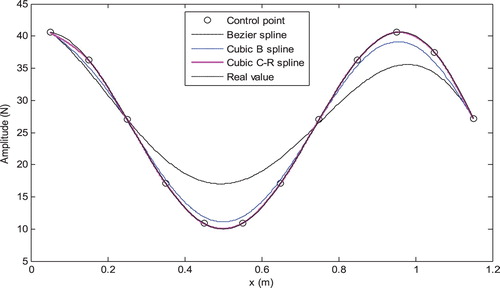
Figure 2 illustrates that cubic Catmull–Rom spline reflects evident superiority compared with the other two kinds of splines in load amplitude interpolation. Primarily, similar to the amplitude of distributed load, three spline curves are all smooth and continuous and there is no mutation in common. Second, the control points represent node amplitudes and they are also part of the entire distributed load spatial course. Simultaneously, cubic Catmull–Rom spline curve can exactly pass through control points and is consistent with real force. Relatively speaking, Bezier spline and cubic B spline both can’t cross over the control points and their precision is lower. In the end, Bezier spline is affected by all control points and has no local property. This means if one or several control points have offset, the interpolation result by Bezier spline will exist massive distortion. While cubic Catmull–Rom spline overcomes this shortcoming. For a Catmull–Rom spline between any two control points, it is only decided by the four control points nearby. The whole spline will not arise large deviation as some control points are inaccurate.

4. Numerical examples

In this section, three numerical examples of distributed excitation identification are performed to validate proposed method. Specifically speaking, three different forms of distributed loads are respectively exerted on a simple supported inflatable beam. For each example, the number of response sensors is $m=12$. Table 1 shows the physical property of the beam.

Table 1. Simple supported inflatable beam property.

$E$	4GPa
$\mu$	0.3
$\rho$	430 kg/m^3
Length	1200 mm
Outer diameter	100 mm
Thickness	0.1 mm
Inflation pressure	10 kPa

As for each numerical example, initial identification result by Taylor polynomial iteration algorithm is distributed force time histories of 12 nodes. If the time history is simple harmonic form, one can extract its amplitude and angular frequency instead of holding entire time history.

Example 1

In this research, the distributed dynamic load can be expressed as a sine form: (26) $f_1\left(x,t\right)=A_1\cdot \sin \left({\omega }_1\cdot t\right).$(26) In Equation (26), the amplitude $A_1$ gradually changes along the beam while the angular frequency ${\omega }_1$ remains constant, that is: (27) $\left\{\begin{array}{l}{A}_1=40\cos \left(4\pi x\right)+30\cos \left(3\pi x\right)+80\\ {\omega }_1=\pi .\end{array}\right.$(27) For this distributed force, only the amplitude $A_1$ needs to be identified. The identification value and error of $A_1$ are shown in Figure 3.

Figure 3. Load amplitude identification result of example 1. (a) Identification value and (b) Identification relative error.

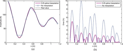
From Figure 3, it can be seen the amplitude values of 12 sensor positions identified by Taylor polynomial iteration algorithm are accurate. But connecting these 12 values directly will lead to a certain offset compared to real distributed force. Especially at the inflection of the amplitude curve, the relative error is more obvious. The errors on half of the whole beam exceed 5% and the maximum error reaches 10%. Through cubic Catmull–Rom spline interpolation processing, the amplitude spatial course is much better consistent with real value. And the relative errors along the beam drop to less than 5%. That means cubic Catmull–Rom spline interpolation plays a crucial role for obtaining exact spatial course of distributed load amplitude in this study.

In order to test the noise resistance ability, different levels of white noises are mixed into the measured response. The amplitude $A_1$ is recalculated and the identification result is presented in Figure 4.

Figure 4. Load amplitude identification result of example 1 in different noise levels. (a) Identification value in 5% noise level; (b) Identification error in 5% noise level; (c) Identification value in 10% noise level; (d) Identification error in 10% noise level; (e) Identification value in 15% noise level and (f) Identification error in 15% noise level.

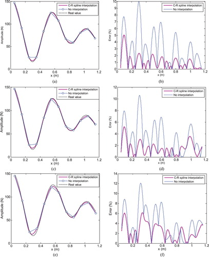
According to Figure 4(a), (c) and (e), the identified node amplitudes have a certain degree of migration compared to the previous condition without noise pollution. The migration will raise with the increase of noise level. After cubic Catmull–Rom spline interpolation, the overall trend of amplitude along the beam is still in good agreement with the real situation. Figure 4(b), (d) and (f) illustrate the identification errors have a rise due to different extents of noises interference. Before interpolation, the largest errors in three noise levels are 10%, 11% and 13%. While the identification error after interpolation is lower in most positions of the beam and no more than 7%.

Example 2

In this case, the distributed force applied on the beam is (28) $f_2\left(x,t\right)=A_2\cdot \sin \left({\omega }_2\cdot t\right).$(28) For $f_2\left(x,t\right)$, the amplitude $A_2$ and angular frequency ${\omega }_2$ both change along the beam, they are expressed as (29) $\left\{\begin{array}{l}{A}_2=20x^3+4x^2+2x+50,\\ {\omega }_2=\sin \left(3\pi x\right)+\cos \left(2\pi x\right)+5.\end{array}\right.$(29) After identifying the distributed force time histories of 12 nodes, the amplitude $A_2$ and angular frequency ${\omega }_2$ are extracted from identification results for the sake of intuition. They are respectively represented as one-dimensional curve graphs in Figures 5 and 6.

Figure 5. Load amplitude identification result of example 2. (a) Identification value and (b) Identification relative error.

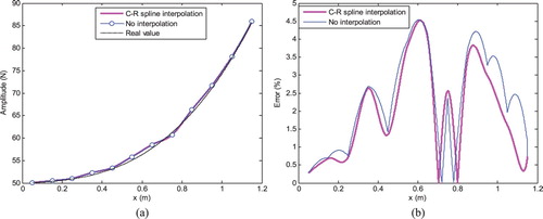
Figure 6. Load angular frequency identification result of example 2. (a) Identification value and (b) Identification relative error.

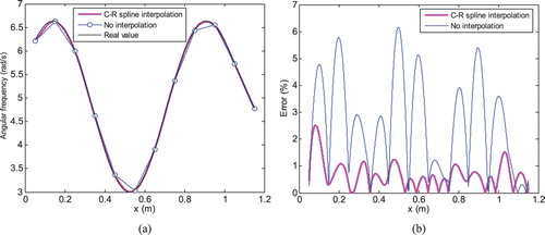
Figure 5 shows the identification results before and after cubic Catmull–Rom spline interpolation are both close to real value. Besides, their identification errors are under 5%. If the amplitude curve is monotonically increasing or decreasing, cubic Catmull–Rom spline interpolation algorithm has no evident assistance for improving the identification precision.

It can be seen in Figure 6 the identification of angular frequency by proposed method fits well with real angular frequency. The relative error keeps below 3%. Cubic Catmull–Rom spline interpolation is indispensable to acquire satisfactory effect.

In the next step, the white noise is added into response signal. The identification results of $A_2$ and ${\omega }_2$ are presented in Figures 7 and 8.

Figure 7. Load amplitude identification result of example 2 in different noise levels. (a) Identification value in 5% noise level; (b) Identification error in 5% noise level; (c) Identification value in 10% noise level; (d) Identification error in 10% noise level; (e) Identification value in 15% noise level and (f) Identification error in 15% noise level.

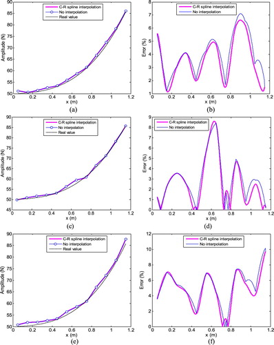
Figure 8. Load angular frequency identification result of example 2 in different noise levels. (a) Identification value in 5% noise level; (b) Identification error in 5% noise level; (c) Identification value in 10% noise level; (d) Identification error in 10% noise level; (e) Identification value in 15% noise level and (f) Identification error in 15% noise level.

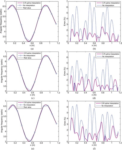
Taking Figure 5 as contrast, Figure 7 displays that external noise will increase the identification error to a certain extent. However, the effect of different levels of noise is not sharp. The value of relative error along the beam is not higher than 10%, which is in an acceptable range.

Compared Figure 8 with Figure 6, the mixed noise makes little difference for angular frequency identification. Relative error doesn’t exceed 4% after interpolation. In this case, the distributed force in a determined node is a sinusoidal time history. The noise only leads to some offset of the amplitude, while the overall trend of sine curve is not affected. Therefore angular frequency has no great variation.

Example 3

The identified distributed load $f_3\left(x,t\right)$ of this example is sine superposition form in each fixed position: (30) $f_3\left(x,t\right)=A_3\left[\sin \left({\omega }_3\cdot t\right)+\sin \left({\omega }_4\cdot t\right)\right].$(30) In Equation (30), $A_3$, ${\omega }_3$ and ${\omega }_4$ all change along the direction of the beam. They are concretely represented in Equation (31): (31) $\left\{\begin{array}{l}{A}_3=20\sin \left(5\pi x\right)+5x^2+3x+1,\\ {\omega }_3=\pi x,\\ {\omega }_4=0.5\pi x.\end{array}\right.$(31) The identification results are expressed as two-dimensional surface images and they are put forward in Figure 9.

Figure 9. Load identification result of example 3. (a) Identification value before interpolation; (b) Identification error before interpolation; (c) Identification value after interpolation and (d) Identification error after interpolation.

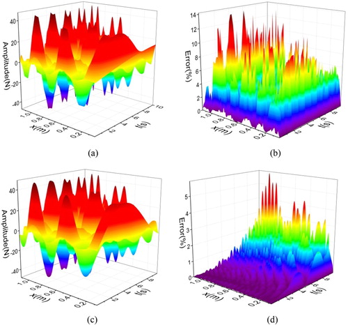
Observing Figure 9, one can realize that the identification result without interpolation has relatively big mistakes. Relative errors of more than half of the identification values exceed 5%. In some positions, the offsets are over 10%. After cubic Catmull–Rom spline interpolation processing in Figure 9, the identification errors have a large drop and lower than 5%. Above data demonstrate that the proposed method is able to achieve satisfactory effect for identifying distributed load of sine superposition form.

In the following procedure, the response is mixed by output noise, then the time history and spatial distribution of distributed force are computed again. Figures 10–12 present the reconstruction results.

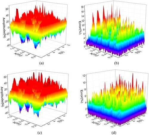
Figures 10(a,b), 11(a,b) and 12(a,b) indicate that noise disturbance will result in an increase of identification error. The higher the noise level is, the larger the relative error becomes. The largest relative error without interpolation is close to 15%. While through cubic Catmull–Rom spline interpolation, the identification errors under 30 and 60 dB down to less than 10% in Figures 10(c,d) and 11(c,d). In Figure 12(c,d) under 90 dB noise level, only a few points exceed 10% of the error and the biggest error is 11%. This condition proves that proposed method can effectively resist environmental noise and keep the stability of identification results.

Figure 10. Load identification result of example 3 in 5% noise level. (a) Identification value before interpolation; (b) Identification error before interpolation; (c) Identification value after interpolation and (d) Identification error after interpolation.

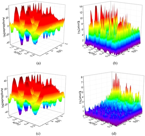
Figure 11. Load identification result of example 3 in 10% noise level. (a) Identification value before interpolation; (b) Identification error before interpolation; (c) Identification value after interpolation and (d) Identification error after interpolation.

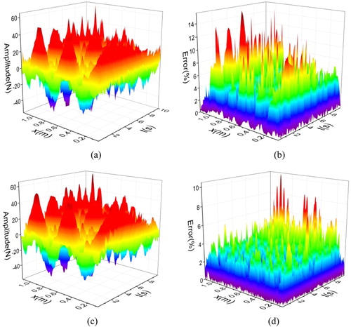
Figure 12. Load identification result of example 3 in 15% noise level. (a) Identification value before interpolation; (b) Identification error before interpolation; (c) Identification value after interpolation and (d) Identification error after interpolation.

5. Conclusion

In this paper, an integrated algorithm which associates Taylor polynomial iteration and cubic Catmull–Rom spline interpolation is put forward to identify distributed forces. Three different numerical cases are implemented to verify the rationality and effectiveness of this method. Identification results before and after spline interpolation operation are contrasted in each example as well.

Compared to previous studies aiming at distributed force identification, this paper has the following highlights and progresses:

1. The whole identification process is carried out in time domain rather than frequency domain. It means this method is able to eliminate the calculation of natural frequencies and natural mode shapes. Meanwhile the error caused by time and frequency conversion is avoided.

2. The integrated method proposed in this paper is able to identify distributed force amplitudes on the whole beam not merely positions of measure points. In particular, Taylor polynomial iteration is applied to compute the distributed excitation amplitudes of measure points. Then these values are taken as control points and cubic Catmull–Rom spline interpolation is performed to reconstruct distributed force spatial curve along the beam.

To sum up, this paper obtains these conclusions:

1. For distributed dynamic loads with different complication degree, proposed method can correctly identify time histories and spatial trends of these distributed forces with a high precision.

2. Cubic Catmull–Rom spline interpolation reveals an evident superiority for distributed load whose amplitude is fluctuant rather than monotonous.

3. In the case that the response is mixed into different levels of noises, identification error maintains in an acceptable range, which illustrates that this method has a strong anti-noise ability.

Disclosure statement

No potential conflict of interest was reported by the authors.

References

- Li J, Hao H. Substructural interface force identification with limited vibration measurements. J Civil Struct Health Monit. 2016;6:395–410. doi: 10.1007/s13349-016-0157-8
- Lage YE, Maia NMM, Neves MM. Force identification using the concept of displacement transmissibility. J Sound Vib. 2013;332:1674–1686. doi: 10.1016/j.jsv.2012.10.034
- Lage YE, Maia NMM, Neves MM. Force magnitude reconstruction using the force transmissibility concept. Shock Vib. 2014; ID: 905912.
- Liu K, Law SS, Zhu XQ, et al. Explicit form of an implicit method for inverse force identification. J Sound Vib. 2014;333:730–744. doi: 10.1016/j.jsv.2013.09.040
- Zhu T, Xiao SN, Yang GW. Force identification in time domain based on dynamic programming. Appl Math Comput. 2014;235:223–234.
- Movahedian B, Boroomand B. Inverse identification of time-harmonic loads acting on thin plates using approximated Green’s functions. Inverse Prob Sci Eng. 2016;24:1475–1493. doi: 10.1080/17415977.2015.1124430
- Mao BY, Xie SL, Zhang XN. Identification of impact load using transient statistical energy analysis method. Int J Appl Electromagn. 2014;45:353–361. doi: 10.3233/JAE-141851
- Qiao BJ, Chen XF, Luo XJ, et al. A novel method for force identification based on the discrete cosine transform. J Vib Acoust. 2015;137, ID: 051012. doi: 10.1115/1.4030616
- Doyle JF. A wavelet deconvolution method for impact force identification. Exp Mech. 1997;37:403–408. doi: 10.1007/BF02317305
- Li Z, Feng ZP, Chu FL. A load identification method based on wavelet multi-resolution analysis. J Sound Vib. 2014;333:381–391. doi: 10.1016/j.jsv.2013.09.026
- Liu J, Han X, Jiang C, et al. Dynamic load identification for uncertain structures based on interval analysis and regularization method. Int J Comput Methods. 2011;8:667–683. doi: 10.1142/S0219876211002757
- Liu J, Sun XS, Han X, et al. Dynamic load identification for stochastic structures based on Gegenbauer polynomial approximation and regularization method. Mech Syst Signal Process. 2015;56:35–54. doi: 10.1016/j.ymssp.2014.10.008
- Liu J, Meng XH, Zhang DQ, et al. An efficient method to reduce ill-posedness for structural dynamic load identification. Mech Syst Signal Process. 2017;95:273–285. doi: 10.1016/j.ymssp.2017.03.039
- Kim Y, Nelson PA. Optimal regularisation for acoustic source reconstruction by inverse methods. J Sound Vib. 2004;275:463–487. doi: 10.1016/j.jsv.2003.06.031
- Sun XS, Liu J, Han X. A new improved regularization method for dynamic load identification. Inverse Prob Sci Eng. 2014;22:1062–1076. doi: 10.1080/17415977.2013.854353
- Gao W, Yu KP, Wu Y. A new method for optimal regularization parameter determination in the inverse problem of load identification. Shock Vib. 2016; ID: 7328969.
- Pan CD, Yu L, Liu HL, et al. Moving force identification based on redundant concatenated dictionary and weighted l1-norm regularization. Mech Syst Signal Process. 2018;98:32–49. doi: 10.1016/j.ymssp.2017.04.032
- Qiao BJ, Zhang XW, Gao JW, et al. Sparse deconvolution for the large-scale ill-posed inverse problem of impact force reconstruction. Mech Syst Signal Process. 2017;83:93–115. doi: 10.1016/j.ymssp.2016.05.046
- Qiao BJ, Zhang XW, Wang CX, et al. Sparse regularization for force identification using dictionaries. J Sound Vib. 2016;368:71–86. doi: 10.1016/j.jsv.2016.01.030
- Liu Y, Shepard Jr WS. An improved method for the reconstruction of a distributed force acting on a vibrating structure. J Sound Vib. 2006;291:369–387. doi: 10.1016/j.jsv.2005.06.013
- Djamaa MC, Ouelaaa N, Pezerat C, et al. Reconstruction of a distributed force applied on a thin cylindrical shell by an inverse method and spatial filtering. J Sound Vib. 2007;301:560–575. doi: 10.1016/j.jsv.2006.10.021
- Jiang XQ, Hu HY. Reconstruction of distributed dynamic loads on an Euler beam via mode-selection and consistent spatial expression. J Sound Vib. 2008;316:122–136. doi: 10.1016/j.jsv.2008.02.038
- Jiang XQ, Hu HY. Reconstruction of distributed dynamic loads on a thin plate via mode-selection and consistent spatial expression. J Sound Vib. 2009;323:626–644. doi: 10.1016/j.jsv.2009.01.008
- Li K, Liu J, Han X, et al. Distributed dynamic load identification based on shape function method and polynomial selection technique. Inverse Prob Sci Eng. 2017;25:1323–1342. doi: 10.1080/17415977.2016.1255740
- Li K, Liu J, Han X, et al. A novel approach for distributed dynamic load reconstruction by space–time domain decoupling. J Sound Vib. 2015;348:137–148. doi: 10.1016/j.jsv.2015.03.009
- Lourens E, Fallais DJM. Full-field response monitoring in structural systems driven by a set of identified equivalent forces. Mech Syst Signal Process. 2019;114:106–119. doi: 10.1016/j.ymssp.2018.05.014
- Amiri AK, Bucher C. A procedure for in situ wind load reconstruction from structural response only based on field testing data. J Wind Eng Ind Aerod. 2017;167:75–86. doi: 10.1016/j.jweia.2017.04.009
- Li XW, Deng ZM. Identification of dynamic loads based on second-order Taylor-series expansion method. Shock Vib. 2016; ID: 6461427.
- Li XW, Zhao HT, Chen Z, et al. Force identification based on a comprehensive approach combining Taylor formula and acceleration transmissibility. Inverse Prob Sci Eng. 2018;26:1612–1632. doi: 10.1080/17415977.2017.1417407
- Derose TD, Barsky BA. Geometric continuity, shape parameters, and geometric constructions for Catmull-Rom splines. ACM Trans. Gr. 1988;7:1–41. doi: 10.1145/42188.42265
- Li JC, Chen S. The cubic ∝-Catmull-Rom spline. Math Comput Appl. 2016;21:1–14.
- Calvetti D, Morigi S, Reichel L, et al. Tikhonov regularization and the L-curve for large discrete ill-posed problems. J Compute Appl Math. 2000;123:423–446. doi: 10.1016/S0377-0427(00)00414-3