Solving inverse nodal problem with spectral parameter in boundary conditions

ABSTRACT

In this study, the inverse Sturm-Liouville problem with spectral parameter in boundary conditions on a finite interval is considered. In fact, we use the nodes as input data and compute the approximation of solution of the inverse nodal Sturm-Liouville problem by the first kind Chebyshev polynomials and apply two methods Chebyshev wavelets and Chebyshev interpolation for solving inverse nodal Sturm-Liouville problem. Finally, the results are explained by presenting the numerical example.

KEYWORDS:

• Sturm-Liouville equation
• inverse problem
• the nodes
• Chebyshev wavelet
• Chebyshev interpolation

AMS SUBJECT CLASSIFICATIONS:

• 34A55
• 34B99

1. Introduction

In this study, we consider the inverse nodal Sturm-Liouville problem with spectral parameter in boundary conditions and use the nodes and the first kind Chebyshev polynomials to calculate the approximate solution. In fact, we apply two methods Chebyshev wavelets and Chebyshev interpolation for solving inverse nodal Sturm-Liouville problem and compare them together by providing the numerical example. Inverse nodal problems have been perused by many authors recently (for example see [1–29]). It seems that McLaughlin [12] was researcher who considered the inverse nodal problems for the first time and got some results about the uniqueness and proved that the potential function in inverse Sturm-Liouville problem can be computed by the nodes.

In [30], Babolian and Fattahzadeh used Chebyshev wavelets method for computing the numerical solution of integral equations by using the first kind Chebyshev polynomials. Also in [31,32], Rashed applied Chebyshev interpolation method to solve the integral-differential and integral equations and showed that the approximate solution of these type equations can be calculated by Chebyshev interpolation method.

In this study, we show that the solution of inverse nodal Sturm-Liouville problem can be the solution of an integral equation and offer Chebyshev wavelets and Chebyshev interpolation methods to obtain the approximation of solution of inverse nodal Sturm-Liouville problem.

Furthermore in all studies on inverse nodal problems, the researchers proved the uniqueness of the potential function by a dense set of nodes. In this study, we show that the approximation of inverse nodal problem solution can be calculated with a finite number of nodes by presenting the numerical example.

We consider the equation (1) $-y^{\mathrm{\prime \prime }}+q\left(x\right)y=\lambda y,0<x<1,$(1) with the boundary conditions (2) $\begin{array}{rl}U\left(y\right)& :=y^{\mathrm{\prime }}(0,\lambda )-hy(0,\lambda )=0,\end{array}$(2) (3) $\begin{array}{rl}V\left(y\right)& :=(\lambda -H_1)y^{\mathrm{\prime }}(1,\lambda )+(\lambda H-H_2)y(1,\lambda )=0,\end{array}$(3) where the potential $q\left(x\right)$ is a real function and integrable on $(0,1)$, $\lambda ={\rho }^2$, λ is the spectral parameter, $h,H,H_1,H_2$ are real parameters and $r:=H{H}_1-H_2>0.$

In Section 2, we show the asymptotic form of eigenvalues and the nodes of problem (1(1) $-y^{\mathrm{\prime \prime }}+q\left(x\right)y=\lambda y,0<x<1,$(1) )–(3(3) $\begin{array}{rl}V\left(y\right)& :=(\lambda -H_1)y^{\mathrm{\prime }}(1,\lambda )+(\lambda H-H_2)y(1,\lambda )=0,\end{array}$(3) ) and present the uniqueness theorem for the inverse nodal problem solution. In Section 3, we use Chebyshev wavelets and Chebyshev interpolation methods for approximating the potential $q\left(x\right)$ as the solution of inverse Sturm-Liouville problem and illustrate the obtained results by presenting the numerical example in Section 4.

2. Preliminaries

In this section, we produce the asymptotic form of eigenvalues and nodes of the boundary value problem (1(1) $-y^{\mathrm{\prime \prime }}+q\left(x\right)y=\lambda y,0<x<1,$(1) )–(3(3) $\begin{array}{rl}V\left(y\right)& :=(\lambda -H_1)y^{\mathrm{\prime }}(1,\lambda )+(\lambda H-H_2)y(1,\lambda )=0,\end{array}$(3) ) and present the uniqueness theorem for the inverse nodal problem under the boundary conditions given.

Let ${\lambda }_0<{\lambda }_1<\cdots \to \mathrm{\infty }$ be the eigenvalues of the problem (1(1) $-y^{\mathrm{\prime \prime }}+q\left(x\right)y=\lambda y,0<x<1,$(1) )–(3(3) $\begin{array}{rl}V\left(y\right)& :=(\lambda -H_1)y^{\mathrm{\prime }}(1,\lambda )+(\lambda H-H_2)y(1,\lambda )=0,\end{array}$(3) ) and $0<x_1^n<\cdots <x_{n-1}^n<1,$ be the nodes of nth eigenfunction. In addition, we denote $x_0^n=0$ and $x_n^n=1$.

The solution of Equation (1(1) $-y^{\mathrm{\prime \prime }}+q\left(x\right)y=\lambda y,0<x<1,$(1) ) with the initial conditions $\varphi (0,\lambda )=1,$ ${\varphi }^{\mathrm{\prime }}(0,\lambda )=h,$ can be written in the following form (see [33,34]) $\varphi (x,\lambda )=\cos \rho x+\frac{1}{\rho }{q}_1\left(x\right)\sin \rho x+\frac{1}{2\rho }{\int }_0^{x}q\left(t\right)\sin \rho (x-2t)\mathrm{d}t+O\left(\frac{1}{{\rho }^2}\right),$ where $q_1\left(x\right)=h+\frac{1}{2}{\int }_0^{x}q\left(t\right)\mathrm{d}t.$ Integration by parts results ${\int }_0^{x}q\left(t\right)\sin \rho (x-2t)\mathrm{d}t=-\frac{1}{2\rho }q\left(x\right)\cos \rho x+\frac{1}{2\rho }q\left(0\right)\cos \rho x,$ therefore (4) $\varphi (x,\lambda )=\cos \rho x+\frac{1}{\rho }{q}_1\left(x\right)\sin \rho x+O\left(\frac{1}{{\rho }^2}\right).$(4) We can write (see [33,34]) (5) $\begin{array}{rl}\mathrm{\Delta }\left(\lambda \right)& :=V\left(\varphi \right)=(\lambda -H_1){\varphi }^{\mathrm{\prime }}(1,\lambda )+(\lambda H-H_2)\varphi (1,\lambda )\\ & =-{\rho }^3\sin \rho +{\rho }^2\omega \cos \rho +{\rho }^{2}I\left(\rho \right),\end{array}$(5) where $I\left(\rho \right)=\frac{1}{2}{\int }_0^{1}q\left(t\right)\cos \rho (1-2t)\mathrm{d}t+O\left(\frac{1}{\rho }\right).$ Using the formula (5(5) $\begin{array}{rl}\mathrm{\Delta }\left(\lambda \right)& :=V\left(\varphi \right)=(\lambda -H_1){\varphi }^{\mathrm{\prime }}(1,\lambda )+(\lambda H-H_2)\varphi (1,\lambda )\\ & =-{\rho }^3\sin \rho +{\rho }^2\omega \cos \rho +{\rho }^{2}I\left(\rho \right),\end{array}$(5) ), we have (6) $\begin{array}{rl}{\rho }_n& =(n-1)\pi +\frac{\omega }{n\pi }+o\left(\frac{1}{n}\right),\\ \omega & =h+H+\frac{1}{2}{\int }_0^{1}q\left(t\right)\mathrm{d}t.\end{array}$(6)

Theorem 2.1

Let the Equation (1(1) $-y^{\mathrm{\prime \prime }}+q\left(x\right)y=\lambda y,0<x<1,$(1) ) under the initial conditions (7) $y(0,\lambda )=1,y^{\mathrm{\prime }}(0,\lambda )=h,$(7) be given. Then, the nodes of problem (1(1) $-y^{\mathrm{\prime \prime }}+q\left(x\right)y=\lambda y,0<x<1,$(1) )–(3(3) $\begin{array}{rl}V\left(y\right)& :=(\lambda -H_1)y^{\mathrm{\prime }}(1,\lambda )+(\lambda H-H_2)y(1,\lambda )=0,\end{array}$(3) ) and the length of nodes are formulated in the form of (8) $\begin{array}{rl}{x}_j^n& =\frac{j-\frac{1}{2}}{n-1}-\frac{\omega x_j^n}{n(n-1){\pi }^2}+\frac{q_1\left(x_j^n\right)}{(n-1{)}^2{\pi }^2}+O\left(\frac{1}{n^3}\right),\end{array}$(8) (9) $\begin{array}{rl}{l}_j^n& =\frac{1}{n-1}-\frac{\omega l_j^n}{n(n-1){\pi }^2}+\frac{1}{2(n-1{)}^2{\pi }^2}{\int }_{x_j^n}^{x_{j+1}^n}q\left(t\right)\mathrm{d}t+O\left(\frac{1}{n^3}\right),\end{array}$(9) where $\begin{array}{rl}\omega & =h+H+\frac{1}{2}{\int }_0^{1}q\left(t\right)\mathrm{d}t,\\ q_1\left(x_j^n\right)& =h+\frac{1}{2}{\int }_0^{x_j^n}q\left(t\right)\mathrm{d}t.\end{array}$

Proof.

We have from (4(4) $\varphi (x,\lambda )=\cos \rho x+\frac{1}{\rho }{q}_1\left(x\right)\sin \rho x+O\left(\frac{1}{{\rho }^2}\right).$(4) ) $\varphi (x,\lambda )=\cos \rho x+\frac{1}{\rho }{q}_1\left(x\right)\sin \rho x+O\left(\frac{1}{{\rho }^2}\right),$ where $q_1\left(x\right)=h+\frac{1}{2}{\int }_0^{x}q\left(t\right)\mathrm{d}t.$ Since the nodes $\left\{x_j^n\right\},$ $n>1,$ $j=\overline{1,n-1},$ are the zeroes of nth eigenfunction, we can set $\varphi (x_j^n,{\lambda }_n)=0.$ Thus, $\cos {\rho }_n{x}_j^n+\frac{1}{{\rho }_n}{q}_1\left(x_j^n\right)\sin {\rho }_n{x}_j^n+O\left(\frac{1}{{\rho }_n^2}\right)=0.$ Using formula (6(6) $\begin{array}{rl}{\rho }_n& =(n-1)\pi +\frac{\omega }{n\pi }+o\left(\frac{1}{n}\right),\\ \omega & =h+H+\frac{1}{2}{\int }_0^{1}q\left(t\right)\mathrm{d}t.\end{array}$(6) ), we can write $\begin{array}{rl}& \cos (n-1)\pi x_j^n-\frac{\omega x_j^n}{n\pi }\sin (n-1)\pi x_j^n\\ & +\frac{1}{(n-1)\pi }{q}_1\left(x_j^n\right)(\sin (n-1)\pi x_j^n+\frac{\omega x_j^n}{n\pi }\cos (n-1\left)\pi x_j^n\right)+O\left(\frac{1}{n^2}\right)=0.\end{array}$ Then $\cot (n-1)\pi x_j^n-\frac{\omega x_j^n}{n\pi }+\frac{1}{(n-1)\pi }{q}_1\left(x_j^n\right)+O\left(\frac{1}{n^2}\right)=0.$ Applying Taylor's expansion for the arccot as $n\to \mathrm{\infty }$, we get $x_j^n=\frac{j-\frac{1}{2}}{n-1}-\frac{\omega x_j^n}{n(n-1){\pi }^2}+\frac{q_1\left(x_j^n\right)}{(n-1{)}^2{\pi }^2}+O\left(\frac{1}{n^3}\right).$ Also, the nodal length is $l_j^n=x_{j+1}^n-x_j^n,$ therefore $l_j^n=\frac{1}{n-1}-\frac{\omega l_j^n}{n(n-1){\pi }^2}+\frac{1}{2(n-1{)}^2{\pi }^2}{\int }_{x_j^n}^{x_{j+1}^n}q\left(t\right)\mathrm{d}t+O\left(\frac{1}{n^3}\right).$ Also see [21,22].

Theorem 2.2

The potential $q-\frac{1}{2}{\int }_0^{1}q$ and the parameters h and $(H_2-\lambda H)/(\lambda -H_1)$ are uniquely ascertained by any dense subset of the nodes in $(0,1)$.

Proof.

Similar to the process used to prove the uniqueness theorem in [6,28], this theorem can be proved easily.

Corollary 2.3

The potential function q of the boundary value problem (1(1) $-y^{\mathrm{\prime \prime }}+q\left(x\right)y=\lambda y,0<x<1,$(1) )–(3(3) $\begin{array}{rl}V\left(y\right)& :=(\lambda -H_1)y^{\mathrm{\prime }}(1,\lambda )+(\lambda H-H_2)y(1,\lambda )=0,\end{array}$(3) ) is uniquely ascertained by a dense set of the nodes and the constant $\omega =h+H+\frac{1}{2}{\int }_0^{1}q\left(t\right)\mathrm{d}t.$

Proof.

Similar to [6,13,14], we consider two Sturm-Liouville problems (1(1) $-y^{\mathrm{\prime \prime }}+q\left(x\right)y=\lambda y,0<x<1,$(1) )–(3(3) $\begin{array}{rl}V\left(y\right)& :=(\lambda -H_1)y^{\mathrm{\prime }}(1,\lambda )+(\lambda H-H_2)y(1,\lambda )=0,\end{array}$(3) ) with the potential functions q, $\tilde{q}$ and the nodal points $x_j^n$, ${\tilde{x}}_j^n$ as $x_j^n={\tilde{x}}_j^n,$ $j=\overline{1,n-1},$ $n>1.$ In addition, we suppose that $\omega =\tilde{\omega }$. Then, using formula (6(6) $\begin{array}{rl}{\rho }_n& =(n-1)\pi +\frac{\omega }{n\pi }+o\left(\frac{1}{n}\right),\\ \omega & =h+H+\frac{1}{2}{\int }_0^{1}q\left(t\right)\mathrm{d}t.\end{array}$(6) ), we have ${\rho }_n={\tilde{\rho }}_n$ and consequently ${\lambda }_n={\tilde{\lambda }}_n$. Also, according to Theorem 2.2, we have $(H_2-{\lambda }_{n}H)/({\lambda }_n-H_1)=({\tilde{H}}_2-{\lambda }_n\tilde{H})/({\lambda }_n-{\tilde{H}}_1)$, thus, $-H{\lambda }_n^2+(H_2+H{\tilde{H}}_1){\lambda }_n-{\tilde{H}}_1{H}_2=-\tilde{H}{\lambda }_n^2+{\lambda }_n({\tilde{H}}_2+\tilde{H}{H}_1)-H_1{\tilde{H}}_2.$ Then, we can write $H=\tilde{H},\frac{H_2}{{\tilde{H}}_2}=\frac{H_1}{{\tilde{H}}_1}=K,H_2+H{\tilde{H}}_1={\tilde{H}}_2+\tilde{H}{H}_1.$ By choosing K=1, the above relations are stablished and then we obtain $H_1=\widetilde{H_1},H_2=\widetilde{H_2}.$ Since $\omega =\tilde{\omega }$, $H=\tilde{H}$ and according to Theorem 2.2, $h=\tilde{h}$, then we have ${\int }_0^{1}q={\int }_0^1\tilde{q}$ and consequently by using Theorem 2.2, we get $q=\tilde{q}$ almost everywhere on (0,1).

3. Numerical solution of the inverse nodal problem

In this section, we consider the inverse nodal problem below.

Inverse nodal problem. Given the nodes $\left\{x_j^n\right\},$ construct the potential $q\left(x\right).$

Since the nodes $\left\{x_j^n\right\},$ are the zeroes of the nth eigenfunction $\varphi (x,{\lambda }_n)$, then, we can write $\varphi (x_j^n,{\lambda }_n)=0,j=\overline{1,n-1},n>1.$ Thus, using (4(4) $\varphi (x,\lambda )=\cos \rho x+\frac{1}{\rho }{q}_1\left(x\right)\sin \rho x+O\left(\frac{1}{{\rho }^2}\right).$(4) ), we get (10) ${\int }_0^{x_j^n}q\left(t\right)\mathrm{d}t\cong -2{\rho }_n\cot {\rho }_n{x}_j^n-2h.$(10) The equation mentioned above is the first kind Fredholm integral equation. To calculate the solution of inverse problem, it is sufficient that we get the solution of integral equation mentioned above. We approximate the potential q by the first kind Chebyshev polynomials as the basic functions and convert the integral equation (10) to the system of linear equations. For approximating the potential q, we use two methods Chebyshev wavelets and Chebyshev interpolation.

3.1. Chebyshev wavelets method

Consider following Chebyshev wavelets on the interval $[0,1)$ as [30] ${\psi }_{l,m}\left(t\right)=\left\{\begin{array}{ll}{2}^{k/2}{\tilde{T}}_m(2^{k}t-2l+1),& \frac{l-1}{2^{k-1}}\le t<\frac{l}{2^{k-1}},\\ 0,& \text{otherwise,}\end{array}\right.$ where ${\tilde{T}}_m\left(t\right)=\left\{\begin{array}{ll}\frac{1}{\sqrt{\pi }},& m=0,\\ \sqrt{\frac{2}{\pi }}{T}_m\left(t\right),& m>0,\end{array}\right.$ and $m=0,1,\dots ,M-1,$ $l=1,2,\dots ,2^{k-1},$ k can be any positive integer and the functions $T_m\left(t\right)$ are the first kind Chebyshev polynomials of degree m on the interval $[-1,1]$ gotten by the recursive formula below: $\begin{array}{rl}& T_0\left(t\right)=1,T_1\left(t\right)=t,\\ & T_{m+1}\left(t\right)=2t{T}_m\left(t\right)-T_{m-1}\left(t\right),m=1,2,\dots .\end{array}$ A function $f\left(t\right)$ on the interval $[0,1)$ is expressed as $f\left(t\right)\cong \sum _{l=1}^{2^{k-1}}\sum _{m=0}^{M-1}{c}_{l,m}{\psi }_{l,m}\left(t\right)=C^{\mathrm{T}}\psi \left(t\right),$ where $\begin{array}{rl}C& =[c_{10},c_{11},\dots ,c_{1(M-1)},c_{20},\dots ,c_{2(M-1)},\dots ,c_{2^{k-1}0},\dots ,c_{2^{k-1}(M-1)}{]}^{\mathrm{T}},\\ \mathrm{\Psi }\left(t\right)& =\left[{\psi }_{10}\right(t),\dots ,{\psi }_{1(M-1)}(t),{\psi }_{20}(t),\dots ,{\psi }_{2(M-1)}(t),\dots ,\\ & \times {\psi }_{2^{k-1}0}\left(t\right),\dots ,{\psi }_{2^{k-1}(M-1)}\left(t\right){]}^{\mathrm{T}}.\end{array}$ We approximate the potential $q\left(t\right)$ by Chebyshev wavelets and have (11) $q\left(t\right)\cong \sum _{l=1}^{2^{k-1}}\sum _{m=0}^{M-1}{c}_{l,m}{\psi }_{l,m}\left(t\right).$(11) Substituting (11(11) $q\left(t\right)\cong \sum _{l=1}^{2^{k-1}}\sum _{m=0}^{M-1}{c}_{l,m}{\psi }_{l,m}\left(t\right).$(11) ) into (10(10) ${\int }_0^{x_j^n}q\left(t\right)\mathrm{d}t\cong -2{\rho }_n\cot {\rho }_n{x}_j^n-2h.$(10) ), we obtain $\sum _{l=1}^{2^{k-1}}\sum _{m=0}^{M-1}{c}_{l,m}\left({\int }_0^{x_j^n}{\psi }_{l,m}\left(t\right)\mathrm{d}t\right)\cong -2{\rho }_n\cot {\rho }_n{x}_j^n-2h,n>1,j=\overline{1,n-1}.$ Now, Let the nodal points $\left\{x_j^n\right\},$ be given. The solution of inverse nodal problem can be calculated by using the steps below:

1. Choose k, M. Then set $n=2^{k-1}M+1$.

2. Compute the unknown vector C by applying the linear system below: $AC=B,$ where $A=\left(\begin{array}{ccccccccccc}{a}_{10}^1& a_{11}^1& \cdots & a_{1(M-1)}^1& a_{20}^1& \cdots & a_{2(M-1)}^1& \cdots & a_{2^{k-1}0}^1& \cdots & a_{2^{k-1}(M-1)}^1\\ a_{10}^2& a_{11}^2& \cdots & a_{1M}^1& a_{20}^2& \cdots & a_{2(M-1)}^2& \cdots & a_{2^{k-1}0}^2& \cdots & a_{2^{k-1}(M-1)}^2\\ .& & & & & .& & & & & .\\ .& & & & & .& & & & & .\\ .& & & & & .& & & & & .\\ a_{10}^{m^{\mathrm{\prime }}}& a_{11}^{m^{\mathrm{\prime }}}& \cdots & a_{1(M-1)}^{m^{\mathrm{\prime }}}& a_{20}^{m^{\mathrm{\prime }}}& \cdots & a_{2(M-1)}^{m^{\mathrm{\prime }}}& \cdots & a_{2^{k-1}0}^{m^{\mathrm{\prime }}}& \cdots & a_{2^{k-1}(M-1)}^{m^{\mathrm{\prime }}}\\ & & & & & & & & & & \end{array}\right)$ where $\begin{array}{rl}& a_{l,m}^j={\int }_0^{x_j^n}{\psi }_{l,m}\left(t\right)\mathrm{d}t,\\ & l=\overline{1,2^{k-1}},m=\overline{0,M-1},n=2^{k-1}M+1,j=\overline{1,n-1},m^{\mathrm{\prime }}=2^{k-1}M,\end{array}$ and $\begin{array}{rl}B& =\left(\begin{array}{c}-2{\rho }_n\cot {\rho }_n{x}_1^n-2h\\ -2{\rho }_n\cot {\rho }_n{x}_2^n-2h\\ .\\ .\\ .\\ -2{\rho }_n\cot {\rho }_n{x}_{n-1}^n-2h\end{array}\right),\\ C& =[c_{10},c_{11},\dots ,c_{1(M-1)},c_{20},\dots ,c_{2(M-1)},\dots ,c_{2^{k-1}0},\dots ,c_{2^{k-1}(M-1)}{]}^{\mathrm{T}}.\end{array}$

3. Find the approximate values $q\left(t_i\right),$ $i=\overline{1,m^{\mathrm{\prime }}}$ by using the following formula $\left[q\right(t_i\left)\right]=C^{\mathrm{T}}\mathrm{\Phi },$ where $t_i=\frac{2i-1}{2^{k}M},i=1,2,\dots ,2^{k-1}M,$ and $\mathrm{\Phi }=\left[\psi \left(\frac{1}{2m^{\mathrm{\prime }}}\right),\psi \left(\frac{3}{2m^{\mathrm{\prime }}}\right),\dots ,\psi \left(\frac{2m^{\mathrm{\prime }}-1}{2m^{\mathrm{\prime }}}\right)\right],m^{\mathrm{\prime }}=2^{k-1}M.$

3.2. Chebyshev interpolation method

By using Chebyshev interpolation technique for the function $q\left(t\right)$, one can show [31,32] that (12) $q\left(t\right)\cong \sum _{i=0}^N{q}_i{l}_{i,N}\left(t\right),t\in (0,1),$(12) where $\begin{array}{rl}{l}_{i,N}\left(t\right)& =\frac{2{\delta }_i}{N}{\sum _{k=0}^N}^{\mathrm{\prime \prime }}{T}_k(2t-1)\cos \left(\frac{ki\pi }{N}\right),\\ {\delta }_i& =\left\{\begin{array}{ll}0.5& i=0,N,\\ 1& 0<i<N,\end{array}\right.\end{array}$ and the numbers $q_i,$ $i=\overline{0,N}$ exist the values of potential function $q\left(t\right)$ in the points $t_i=(\cos (i\pi /N)+1)/2$ which are the extrema of $T_N(2t-1)$. In addition, $\sum ^{\mathrm{\prime \prime }}$ is the sum of all terms except the first and last two sentences so that the sum of half of the two sentences is considered.

Substituting (12(12) $q\left(t\right)\cong \sum _{i=0}^N{q}_i{l}_{i,N}\left(t\right),t\in (0,1),$(12) ) into (10(10) ${\int }_0^{x_j^n}q\left(t\right)\mathrm{d}t\cong -2{\rho }_n\cot {\rho }_n{x}_j^n-2h.$(10) ) with $n\ge 1$, we have $\begin{array}{rl}& \sum _{i=0}^N{q}_i\frac{2{\delta }_i}{N}{\sum _{k=0}^N}^{\mathrm{\prime \prime }}\left({\int }_0^{x_j^n}{T}_k(2t-1)\mathrm{d}t\right)\cos \left(\frac{ki\pi }{N}\right)\\ & \cong -2{\rho }_n\cot {\rho }_n{x}_j^n-2h,n>1.\end{array}$ Denote $g\left(x_j^n\right)=-2{\rho }_n\cot {\rho }_n{x}_j^n-2h,$ $n>1,$ and $\begin{array}{rl}{I}_k\left(x_j^n\right)& ={\int }_0^{x_j^n}{T}_k(2t-1)\mathrm{d}t,\\ R(t_i,x_j^n)& =\frac{2{\delta }_i}{N}{\sum _{k=0}^N}^{\mathrm{\prime \prime }}{I}_k\left(x_j^n\right)\cos \left(\frac{ki\pi }{N}\right).\end{array}$ Using the above formulas, we have $\sum _{i=0}^{N}R(t_i,x_j^n)q_i\cong g\left(x_j^n\right),n>1.$ Now, Let the nodal points $\left\{x_j^n\right\},$ be given. Then, the solution of inverse nodal problem can be calculated by using the following steps:

1. Choose n and set $N=n-2.$

2. Find the coefficients $q_i,$ $i=\overline{0,N}$ by the linear system below: $A\hat{q}=B,$ where $\hat{q}=[q_0{q}_1\cdots q_N{]}^{\mathrm{T}},$ $\begin{array}{rl}A& =\left(\begin{array}{cccccc}R(t_0,x_1^n)& R(t_1,x_1^n)& .& .& .& R(t_N,x_1^n)\\ R(t_0,x_2^n)& R(t_1,x_2^n)& .& .& .& R(t_N,x_2^n)\\ .& .& & .& & .\\ .& .& & .& & .\\ .& .& & .& & .\\ R(t_0,x_{n-1}^n)& R(t_1,x_{n-1}^n)& .& .& .& R(t_N,x_{n-1}^n)\\ & & & & & \end{array}\right)\\ & =\left(\begin{array}{cccccc}\frac{1}{N}{\sum _{k=0}^N}^{\mathrm{\prime \prime }}{I}_k\left(x_1^n\right)& \frac{2}{N}{\sum _{k=0}^N}^{\mathrm{\prime \prime }}{I}_k\left(x_1^n\right)\cos \left(\frac{k\pi }{N}\right)& .& .& .& \frac{1}{N}{\sum _{k=0}^N}^{\mathrm{\prime \prime }}(-1{)}^k{I}_k(x_1^n)\\ \frac{1}{N}{\sum _{k=0}^N}^{\mathrm{\prime \prime }}{I}_k\left(x_2^n\right)& \frac{2}{N}{\sum _{k=0}^N}^{\mathrm{\prime \prime }}{I}_k\left(x_2^n\right)\cos \left(\frac{k\pi }{N}\right)& .& .& .& \frac{1}{N}{\sum _{k=0}^N}^{\mathrm{\prime \prime }}(-1{)}^k{I}_k(x_2^n)\\ .& .& & .& & .\\ .& .& & .& & .\\ .& .& & .& & .\\ \frac{1}{N}{\sum _{k=0}^N}^{\mathrm{\prime \prime }}{I}_k\left(x_{n-1}^n\right)& \frac{2}{N}{\sum _{k=0}^N}^{\mathrm{\prime \prime }}{I}_k\left(x_{n-1}^n\right)\cos \left(\frac{k\pi }{N}\right)& .& .& .& \frac{1}{N}{\sum _{k=0}^N}^{\mathrm{\prime \prime }}(-1{)}^k{I}_k(x_{n-1}^n)\\ & & & & & \end{array}\right),\end{array}$where $I_k\left(x_m^n\right)={\int }_0^{x_m^n}{T}_k(2t-1)\mathrm{d}t.$ Moreover $B=\left(\begin{array}{c}g\left(x_1^n\right)\\ g\left(x_2^n\right)\\ .\\ .\\ .\\ g\left(x_{n-1}^n\right)\end{array}\right)=\left(\begin{array}{c}-2{\rho }_n\cot {\rho }_n{x}_1^n-2h\\ -2{\rho }_n\cot {\rho }_n{x}_2^n-2h\\ .\\ .\\ .\\ -2{\rho }_n\cot {\rho }_n{x}_{n-1}^n-2h\end{array}\right).$

3. Calculate the potential function q by using the formula (12(12) $q\left(t\right)\cong \sum _{i=0}^N{q}_i{l}_{i,N}\left(t\right),t\in (0,1),$(12) ).

4. Numerical example

In this section, we use the methods presented in this study to solve inverse nodal problem (1(1) $-y^{\mathrm{\prime \prime }}+q\left(x\right)y=\lambda y,0<x<1,$(1) )–(3(3) $\begin{array}{rl}V\left(y\right)& :=(\lambda -H_1)y^{\mathrm{\prime }}(1,\lambda )+(\lambda H-H_2)y(1,\lambda )=0,\end{array}$(3) ) and provide a numerical example to show the accuracy of presented methods. The calculations associated with the example presented in this section are performed using Matlab software program.

Example 4.1

Consider the potential $q\left(x\right)=\sin \left(3\pi x\right)$ and h=H=1. The numerical values of nodes $x_j^n,$ $n=13,$ $j=\overline{1,12}$ can be computed by the formula (8(8) $\begin{array}{rl}{x}_j^n& =\frac{j-\frac{1}{2}}{n-1}-\frac{\omega x_j^n}{n(n-1){\pi }^2}+\frac{q_1\left(x_j^n\right)}{(n-1{)}^2{\pi }^2}+O\left(\frac{1}{n^3}\right),\end{array}$(8) ) seen in Table 1. Now, we suppose that the nodes given in Table 1 are the input data and q is the unknown function in inverse nodal problem. We get the approximation of potential q as the solution of inverse nodal problem by using Chebyshev wavelet method and Chebyshev interpolation method. The results gotten in this example with k=M=3 and n=13 are seen in Table 2 where q and $\tilde{q}$ denote the exact and approximate solutions, respectively. In Table 2, It is clear that Chebyshev interpolation method compared with Chebyshev wavelet method is more accurate. Finally, we draw the numerical approximation obtained with $k=4,$ M=7 and n=57 and exact solution by using Chebyshev wavelet method shown in Figure 1. It is seen that for large n, wavelet Chebyshev method is a good method for solving the inverse nodal Sturm-Liouville problems.

Figure 1. Approximate and exact solutions of inverse nodal problem using Chebyshev wavelet method in Example 4.1 with n=57: (***) for the exact solution and (- - -) for the approximate solution.

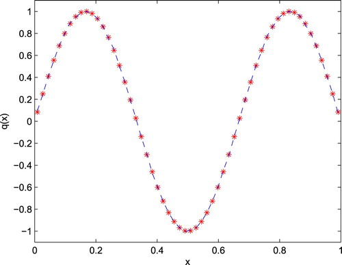
Table 1. Numerical values of nodes $x_j^n$ in Example 4.1 with n=13.

j	1	2	3	4	5	6
$x_j^n$	0.0423161315	0.1255556747	0.2088035859	0.2920431292	0.3752624706	0.4584616101
j	7	8	9	10	11	12
$x_j^n$	0.5416523818	0.6248515214	0.7080708628	0.7913104060	0.8745583172	0.9577978604

Table 2. Absolute error of exact and approximate solutions in Example 4.1.

	Absolute error $|q-\tilde{q}|$	Absolute error $|q-\tilde{q}|$
$t_i$	Chebyshev wavelet method	Chebyshev interpolation method
$0.041\overline{6}$	0.0808023978	0.0279601501
0.1250	0.0575215606	0.0064502819
$0.208\overline{3}$	0.1166642530	0.0012518098
$0.291\overline{6}$	0.1357508823	0.0004014580
0.3750	0.0811187572	0.0048876064
$0.458\overline{3}$	0.2147850235	0.0097981967
$0.541\overline{6}$	0.2225430976	0.0100129764
0.6250	0.1392119313	0.0060319169
$0.708\overline{3}$	0.3067156266	0.0010501754
$0.791\overline{6}$	0.3275786111	0.0004377981
0.8750	0.1679019186	0.0002027071
$0.958\overline{3}$	0.3771055756	0.0403948015

5. Conclusion

In this study, we propounded Sturm-Liouville equation with boundary conditions included spectral parameter. We applied the relationship between the inverse nodal Sturm-Liouville problem and Fredholm integral equation of the first kind and computed the approximate solution of associated inverse problem by Chebyshev wavelet and Chebyshev interpolation methods for the first time. By preparing the numerical example, we showed that both methods were good methods for solving the inverse nodal problems of this form but Chebyshev interpolation method was more accurate compared with Chebyshev wavelet method. Furthermore, in provided example, it could be found that the approximation of potential q was computed with a finite number of nodes.

Disclosure statement

No potential conflict of interest was reported by the authors.

References

- Browne PJ, Sleeman BD. Inverse nodal problem for Sturm-Liouville equation with eigenparameter dependent boundary conditions. Inverse Probl. 1996;12:377–381. doi: 10.1088/0266-5611/12/4/002
- Cheng YH, Chun-Kong L, Tsay J. Remarks on a new inverse nodal problem. J Math Anal Appl. 2000;248:145–155. doi: 10.1006/jmaa.2000.6878
- Cheng YH, Law CK. The inverse nodal problem for Hill's equation. Inverse Probl. 2006;22:891–901. doi: 10.1088/0266-5611/22/3/010
- Gulsen T, Yilmaz E, Akbarpoor Sh. Numerical investigation of the inverse nodal problem by Chebyshev interpolation method. Thermal Sci. 2018;22:S123–S136. doi: 10.2298/TSCI170612278G
- Hald OH, McLaughlin JR. Solution of inverse nodal problems. Inverse Probl. 1989;5:307–347. doi: 10.1088/0266-5611/5/3/008
- Koyunbakan H. A new inverse problem for the diffusion operator. Appl Math Lett. 2006;19:995–999. doi: 10.1016/j.aml.2005.09.014
- Koyunbakan H. Erratum to ‘Inverse nodal problem for differential operator with eigenvalue in the boundary condition’ [Appl Math Lett 21 (2008) 1301–1305]. Appl Math Lett. 2009;22:792–795. doi: 10.1016/j.aml.2008.10.001
- Koyunbakan H, Panakhov ES. Solution of a discontinuous inverse nodal problem on a finite interval. Math Comput Model. 2006;44:204–209. doi: 10.1016/j.mcm.2006.01.012
- Koyunbakan H, Panakhov ES. A uniqueness theorem for inverse nodal problem. Inverse Probl Sci Eng. 2007;12:517–524. doi: 10.1080/00423110500523143
- Law CK, Shen CL, Yang CF. The inverse nodal problem on the smoothness of the potential function. Inverse Probl. 1999;15:253–263. doi: 10.1088/0266-5611/15/1/024
- Law CK, Yang CF. Reconstructing the potential function and its derivatives using nodal data. Inverse Probl. 1998;14:299–312. doi: 10.1088/0266-5611/14/2/006
- McLaughlin JR. Inverse spectral theory using nodal points as data-a uniqueness result. J Differ Equ. 1988;73:342–362. doi: 10.1016/0022-0396(88)90111-8
- Neamaty A, Akbarpoor Sh. Numerical solution of inverse nodal problem with an eigenvalue in the boundary condition. Inverse Probl Sci Eng. 2017;25:978–994. doi: 10.1080/17415977.2016.1209751
- Neamaty A, Akbarpoor Sh, Yilmaz E. Solving inverse Sturm-Liouville problem with separated boundary conditions by using two different input data. Int J Comput Math. 2017. DOI:10.1080/00207160.2017.1346244
- Neamaty A, Yilmaz E, Akbarpoor Sh, et al. Numerical solution of singular inverse nodal problem by using Chebyshev polynomials. Konuralp J Math. 2017;5(2):131–145.
- Rundell W, Sacks PE. The reconstruction of Sturm-Liouville operators. Inverse Probl. 1992;8:457–482. doi: 10.1088/0266-5611/8/3/007
- Shen CL. On the nodal sets of the eigenfunctions of the string equations. SIAM J Math Anal. 1988;19:1419–1424. doi: 10.1137/0519104
- Shen CL, Tsai TM. On a uniform approximation of the density function of a string equation using eigenvalues and nodal points and some related inverse nodal problems. Inverse Probl. 1995;11:1113–1123. doi: 10.1088/0266-5611/11/5/014
- Shieh CT, Yurko VA. Inverse nodal and inverse spectral problems for discontinuous boundary value problems. J Math Anal Appl. 2008;347:266–272. doi: 10.1016/j.jmaa.2008.05.097
- Wang YP. Inverse problems for discontinuous Sturm-Liouville operators with mixed spectral data. Inverse Probl Sci Eng. 2015;23:1180–1198. doi: 10.1080/17415977.2014.981748
- Wang YP, Lien KY, Shieh CT. Inverse problems for the boundary value problem with the interior nodal subsets. Appl Anal. 2017;96:1229–1239. doi: 10.1080/00036811.2016.1183770
- Wang YP, Lien KY, Shieh CT. On a uniqueness theorem of Sturm-Liouville equations with boundary conditions polynomially dependent on the spectral parameter. Bound Value Probl. 2018;28. DOI:10.1186/s13661-018-0948-4
- Wang YP, Shieh CT, Miao HY. Reconstruction for Sturm-Liouville equations with a constant delay with twin-dense nodal subsets. Inverse Probl Sci Eng. 2018. DOI:10.1080/17415977.2018.1489803
- Yang XF. A solution of the inverse nodal problem. Inverse Probl. 1997;13:203–213. doi: 10.1088/0266-5611/13/1/016
- Yang XF. A new inverse nodal problem. J. Differential Equations. 2001;169:633–653. doi: 10.1006/jdeq.2000.3911
- Yang CF. Reconstruction of the diffusion operator from nodal data. Verlag der Zeitschrift für Naturforch. 2010;65a:100–106.
- Yang CF, Yang XP. Inverse nodal problems for the Sturm-Liouville equation with polynomially dependent on the eigenparameter. Inverse Probl Sci Eng. 2011;19(7):951–961. doi: 10.1080/17415977.2011.565874
- Yilmaz E, Koyunbakan H. Reconstruction of potential function and its derivatives for Sturm-Liouville problem with eigenvalues in boundary condition. Inverse Probl Sci Eng. 2010;18:935–944. doi: 10.1080/17415977.2010.492514
- Yilmaz E, Koyunbakan H, Ic U. Inverse nodal problem for the differential operator with a singularity at zero. Comput Model Eng Sci. 2013;92:303–313.
- Babolian E, Fattahzadeh F. Numerical computation method in solving integral equations by using Chebyshev wavelet operational matrix of integration. Appl Math Comput. 2007;188:1016–1022.
- Rashed MT. Numerical solution of a special type of integro-differential equations. Appl Math Comput. 2003;143:73–88.
- Rashed MT. Numerical solutions of the integral equations of the first kind. Appl Math Comput. 2003;145:413–420.
- Dehghani Tazehkand I, Jodayree Akbarfam A. On inverse Sturm-Liouville problems with spectral parameter linearly contained in the boundary conditions. ISRN Math Anal. 2011. DOI:10.5402/2011/754718
- Freiling G, Yurko V. Inverse Sturm-Liouville problems and their applications. New York: NOVA Science Publishers; 2001.