CT image reconstruction algorithms based on the Hanke Raus parameter choice rule

ABSTRACT

Computed tomography (CT) image reconstruction is one of the focal problems in clinical medicine. The data received by the detector is usually not completed for man-made or environmental factors. To reconstruct high-quality CT images from incomplete data, total variation (TV) regularization has shown great potential, in which the choice of the regularization parameter becomes a crucial problem. In this paper, the Hanke Raus rule without the knowledge of noise level is derived and applied to choose the regularization parameter of TV regularization and the split Bregman iteration based on a continuation strategy is utilized to TV minimization. The proposed reconstruction algorithm is applied to limited projection data of the Shepp-Logan phantom image as well as the teeth image. The numerical results demonstrate that the proposed algorithm based on the Hanke Raus rule exhibits superior performance than the sequential discrepancy principle and the L-curve rule.

KEYWORDS:

• Limited projection data
• the Hanke Raus rule
• TV minimization
• split Bregman iteration

2010 MATHEMATICS SUBJECT CLASSIFICATIONS:

• 44A12
• 65N21
• 65R32

1. Introduction

Compared with radiography, computed tomography (CT) can distinguish the anatomical structure and the specific location of lesion more clearly. Therefore, the scope of examination on the human body is enlarged significantly, which improves the recognizable rate of the disease and the accuracy of the diagnosis. Moreover, it is very important in modern clinical diagnosis whether CT image can be reconstructed accurately. Many scholars have paid much attention to this problem.

A simple physical model is reviewed here. $f\left(x\right)$ is the X-ray attenuation coefficient of the tissue at the point x, and the tissue is divided into little blocks with same size along these ray paths l. The process of X-ray going through each block follows the Lambert-Beer law, (1) $I=I_0{\mathrm{e}}^{-{\int }_{l}f\left(x\right)\mathrm{d}x}.$(1) Here I and $I_0$ denote the intensity received by the detector behind the object and the intensity of the ray sent from the X-ray source, respectively. Equation (1(1) $I=I_0{\mathrm{e}}^{-{\int }_{l}f\left(x\right)\mathrm{d}x}.$(1) ) describes the scanning process, that is the line integral of the function f along each of the lines l. We have to reconstruct f from all these integrals.

We model a two-dimensional slice through the target object by a rectangle $\mathrm{\Omega }\subset {\mathbb{R}}^2$, and a nonnegative attenuation coefficient $f:\mathrm{\Omega }\to [0,\mathrm{\infty })$. The object is contained in a subset ${\mathrm{\Omega }}_1\subset \mathrm{\Omega }$, and $f\left(x\right)=0$ for $x\in \mathrm{\Omega }\setminus {\mathrm{\Omega }}_1$. This process can be described by Radon transform as (2) $\begin{array}{rl}& \mathcal{R}:L^2\left(\mathrm{\Omega }\right)\to L^2\left(D\right)\\ & \left(\mathcal{R}f\right)(\theta ,s)={\int }_{L(\theta ,s)}f\left(l\right)\mathrm{d}l\end{array}$(2) where $L(\theta ,s)=\{f\in {\mathbb{R}}^2:f_1\cos \theta +f_2\sin \theta =s\}$ is the line of the X-ray, $D=\left\{\right(\theta ,s):-r\le s\le r,0\le \theta <\pi \}$ is the projection space. This leads to the linear equation (3) $\mathcal{R}f=g,$(3) where the data g on the right side of the equation is the projection or observation value, which usually appears as the sinogram. Therefore, the reconstruction problem of CT simply calls for the inversion of the Radon transformation. In 1917, Johann Radon gave an explicit inversion formula (see section 1.1 in [1]). It has been proven that the Radon transformation $\mathcal{R}$ is compact [1]. Especially, the Radon transform is $L^2$ continuous, $L^1$ continuous and BV continuous for functions with compact support (see [1,2]). The problem is inherently ill-posed in the sense of unstable dependence of the solution on the data. Because of the surrounding environmental factors, instead of exact data g, only noisy observation data $g^{\delta }$ satisfying $\parallel g-g^{\delta }\parallel \le \delta$ with presumably known δ can be obtained usually. On the other hand, due to some reasons, only a limited projection can be received. For example, the projection is obtained by equal-spacing sparse sampling, or by limited view. Thus, with only limited projections (undersampling), the problem will become undetermined and therefore more ill-posed. In order to overcome these difficulties, we need to find some effective regularization methods [3,4]. Several algorithms for CT image reconstruction have been developed, including the analytic reconstruction algorithm (e.g. Filter back-projection, FBP), the algebraic reconstruction technique, (ART, e.g. Kaczmarz's method with its variants), and simultaneous algebraic reconstruction technique [5] (SART, e.g. Landweber method) [6,7]. For limited data, it is difficult to reconstruct high-quality images by the conventional CT image reconstruction algorithms. Especially, FBP requires high completeness of data [1].

TV minimization was used for few-view and limited-angle CT reconstruction [8–11], in which CT reconstruction problem is converted to a optimization problem (4) $\underset{f}{min}{\mathrm{\Phi }}_{\alpha }\left(f\right)=\frac{1}{2}\parallel \mathcal{R}f-g^{\delta }{\parallel }^2+\alpha \parallel f{\parallel }_{TV}.$(4) Here $\alpha >0$ is a regularization parameter and $\parallel \cdot {\parallel }_{TV}$ is the TV penalty to be introduced in detail in Section 2.1. A key problem of all regularization methods for the ill-posed problems is how to choose the regularization parameter appropriately. The regularization parameter α was usually chosen posteriorly by the Morozov discrepancy principle [3], or by a sequential discrepancy principle [12], which depends on the noise level δ. However, such noise level information is usually unknown in reality. There are several heuristic parameter choice rules which do not use the knowledge of noise level, including the generalized cross validation, the L-curve method [13], quasi-optimality criterion [14] and Hanke Raus rule [15]. We notice that Hanke Raus rule has been extended to the general penalty term in Banach spaces [16,17]. It may as well be a parameter choice rule for the optimization problem with TV constraints (4).

Our contribution in this paper are follows: First, the optimal parameter is chosen by Hanke Raus rule due to the unknown noise level in advance, which is the novelty and the interest of this paper. Second, based on the Hanke Raus rule, split Bregman iteration is combined with the continuation technique respectively. To the best of our knowledge, Hanke Raus rule has not been used as parameter choice rule for split Bregman iteration.

Third, we apply the proposed methods to actual clinical CT images of teeth when the clinical data we obtained is incomplete and the noise level is unknown.

The rest of the paper is organized as follows: In Section 2, the discrete setting of Radon transformation is given, the posterior parameter choice rule, such as sequential discrepancy principle, heuristic parameter choice rules such as L-curve rule and the Hanke Raus rule are introduced. In Section 3, the reconstruction methods and the strategy of parameter selection with incomplete CT data are discussed and simulated in Shepp-Logan image reconstruction. Moreover, with Hanke Raus rule, the proposed algorithm is applied to the actual clinical CT images of teeth. Compared with discrepancy principle and L-curve rule, the numerical results show the effectiveness of Hanke Raus rule.

2. Discrete setting and methods

In this section, we describe the discrete problems and introduce the sequential discrepancy principle, the L-curve rule and the Hanke Raus rule. Moreover, we present TV minimization algorithms based on split Bregman iteration.

2.1. Discrete setting

For each $p,q\in {\mathbb{N}}^{\mathbb{+}}$, ${\ell }_1$, ${\ell }_2$ norm are defined by $\parallel f{\parallel }_1=\sum _{i,j}|f_{i,j}|$ and $\parallel f\parallel =\sqrt{\sum _{i,j}|f_{i,j}{|}^2}$ for any $f\in {\mathbb{R}}^{p\times q}$. Let $f_{i,j}$, $i=1,\dots ,m$, $j=1,\dots ,n$ be the discretized image defined on a rectangular grid of size $m\times n$ and $g_{i,j}$, $i=1,\dots ,k$, $j=1,\dots ,l$ be the discretization for an element in the sinogram space $\mathrm{\Sigma }=[0,\pi )\times [-r,r]$, where k and l are the number of angles and lines, respectively. Then the Radon transformation can be discretized by the following map $R:{\mathbb{R}}^{m\times n}\to {\mathbb{R}}^{k\times l}$ For the line $x({\theta }_{\hat{i}},s_{\hat{j}})$, ($\hat{i}=1,\dots k,\hat{j}=1,\dots l$), we can define ${\psi }_{i,j}({\theta }_{\hat{i}},s_{\hat{j}})=\left\{\begin{array}{ll}1,& \text{when the line }x({\theta }_{\hat{i}},s_{\hat{j}})\text{ goes through the pixel }(i,j)\\ 0,& \mathrm{o}\mathrm{t}\mathrm{h}\mathrm{e}\mathrm{r}\mathrm{w}\mathrm{i}\mathrm{s}\mathrm{e},\end{array}\right.$ where $i=1,\dots ,m$ and $j=1,\dots ,n$. By the linearity of the Radon transform, we have the discrete Radon transform $Rf({\theta }_{\hat{i}},s_{\hat{j}})=\sum _{i=1}^m\sum _{j=1}^n{f}_{i,j}\mathcal{R}{\psi }_{i,j}({\theta }_{\hat{i}},s_{\hat{j}})$ where $\mathcal{R}{\psi }_{i,j}({\theta }_{\hat{i}},s_{\hat{j}})$ is equal to the length of the intersection of the projection line with the pixel $(i,j)$.

Note that R is linear and ill-posed, we consider a Tikhonov-type regularization functional with TV constraint (5) ${\mathrm{\Phi }}_{\alpha }\left(f\right)=\frac{1}{2}\parallel Rf-g^{\delta }{\parallel }^2+\alpha \parallel f{\parallel }_{TV}$(5) In this paper, we introduce the ${\ell }_1$ norm of gradient filed (anisotropic TV) represented as $\parallel f{\parallel }_{TV}=\sum _{i=1}^n\sum _{j=1}^m|{\mathrm{\nabla }}_{1}f|+|{\mathrm{\nabla }}_{2}f|,$ where $({\mathrm{\nabla }}_{1}f,{\mathrm{\nabla }}_{2}f)$ is the discrete gradient of f and $\begin{array}{rl}({\mathrm{\nabla }}_{1}f{)}_{i,j}& =\left\{\begin{array}{ll}{f}_{i+1,j}-f_{i,j},& \text{for }i=1,\dots ,n-1;j=1,\dots ,m-1\\ f_{n,j+1}-f_{n,j},& \mathrm{f}\mathrm{o}\mathrm{r}i=n;j=1,\dots ,m-1;\end{array}\right.\\ ({\mathrm{\nabla }}_{2}f{)}_{i,j}& =\left\{\begin{array}{ll}{f}_{i,j+1}-f_{i,j},& \mathrm{f}\mathrm{o}\mathrm{r}i=1,\dots ,n;j=1,\dots ,m-1,\\ f_{i+1,m}-f_{i,m},& \mathrm{f}\mathrm{o}\mathrm{r}i=1,\dots ,n-1;j=m.\end{array}\right.\end{array}$

2.2. Heuristic parameter choice rules

How to select the regularization parameter is crucial for Tikhonov-type regularization methods. It has been discussed in depth for classical quadratic regularization whether in the theoretical analysis or in the numerical implementation. DP rule (the sequential discrepancy principle) is a frequently-used posterior parameter choice rule in the regularization methods. Choose $\alpha \in {\mathrm{\Delta }}_q$, when the condition is satisfied firstly $\parallel R{f}_{\alpha }-g^{\delta }\parallel \le \tau \delta ,\tau >1,$ in which, the regularization parameters α are tested on a logarithmically uniform grid, i.e. ${\mathrm{\Delta }}_q=\{{\alpha }_0{q}^j:j=0,1,\dots ,0<q<1\}.$ with ${\alpha }_0=\parallel R{\parallel }^2$. However, DP rule requires knowledge of the noise level δ in advance, which is unknown beforehand in reality. In practical application, overestimation or underestimation on the noise level, the accuracy of algorithm will have a significant loss.

The L-curve rule is a very popular error-free parameter rule [13], which displays the trade-off between minimizing the residual term and minimizing the constraint term. The method is done by plotting $\parallel f_{\alpha }{\parallel }_{TV}$ versus $\parallel R{f}_{\alpha }-g^{\delta }{\parallel }^2$ in a log-log scale for a range of α values. For a continuous regularization parameter α, we should compute the curve $(\log (\parallel f_{\alpha }{\parallel }_{TV}),\log (\parallel R{f}_{\alpha }-g^{\delta }{\parallel }^2\left)\right)$ and seek the point with maximum curvature, which is called as the ‘L-curve’ corner. In [18] the discrete L-curve and TV-based conjugate gradient method were applied for few-view CT reconstruction of X-ray. However, the L-curve rule still lacks a sound mathematical foundation and criticisms of the L-curve method have been published [3,19].

The Hanke Raus rule as a heuristic parameter choice rule has been proposed for classical Tikhonov regularization as well as several iterative regularization methods [3,15]. It does not require a knowledge of the noisy level δ and still allow some theoretical justification. Now, we give some motivation of the Hanke Raus rule, especially for regularization with general penalty term.

For a convex and weak lower semicontinuous function $\mathrm{\Theta }:{\mathbb{R}}^{m\times n}\to [0,\mathrm{\infty }]$, we seek a minimizer of the functional ${\mathrm{\Phi }}_{\alpha }\left(f\right)=\frac{1}{2}\parallel Rf-g^{\delta }{\parallel }^2+\alpha \mathrm{\Theta }\left(f\right).$ Let $f_{\alpha }$ be the minimizer of ${\mathrm{\Phi }}_{\alpha }\left(f\right)$ with the regularization parameter α. By the Hanke Raus rule regularization parameter is picked for which $\frac{1}{\alpha }\parallel R{f}_{\alpha }-g^{\delta }{\parallel }^2\to min.$ The motivation comes from following error estimates [20]

Theorem 2.1

Assume that $f^{†}$ satisfies $R{f}^{†}=g$ with $\delta =\parallel g^{\delta }-g\parallel$. Let $D_{\xi }\mathrm{\Theta }(f^{\prime },f)$ be the Bregman distance of Θ from f to $f^{\prime }$ with respect to the direction $\xi \in \mathrm{\partial }\mathrm{\Theta }\left(f\right)$. Then there is constant $\rho >0$, such that the following estimates hold $\begin{array}{rl}& D_{\xi }\mathrm{\Theta }(f_{\alpha },f^{†})\le \frac{(\delta +\rho \alpha {)}^2}{2\alpha },\\ & \parallel R{f}_{\alpha }-g^{\delta }\parallel \le \delta +2\rho \alpha .\end{array}$

From Theorem 2.1, we see that $\frac{\parallel R{f}_{\alpha }-g^{\delta }{\parallel }^2}{\alpha }\le \frac{(\delta +2\rho \alpha {)}^2}{\alpha }$ which implies that $\parallel R{f}_{\alpha }-g^{\delta }{\parallel }^2/\alpha$ can be used for error estimation $D_{\xi }\mathrm{\Theta }(f_{\alpha },f^{†})$. Therefore, in the Hanke Raus rule a computable function $H(\alpha ,g^{\delta })$ is defined $H(\alpha ,g^{\delta }):=\frac{\parallel R{f}_{\alpha }-g^{\delta }{\parallel }^2}{\alpha }.$ It can be proved that the function $\alpha \mapsto \parallel R{f}_{\alpha }-g^{\delta }\parallel$ is monotonically increasing and uniformly bounded, which implies that $\underset{\alpha \to +\mathrm{\infty }}{lim}H(\alpha ,g^{\delta })=0$. Therefore, we can get an optimal parameter ${\alpha }_{\ast }$ by minimizing $H(\alpha ,g^{\delta })$ over any bounded and closed interval of $[0,\mathrm{\infty }]$.

In [16], the authors also derived the error estimates, when the optimal parameter ${\alpha }_{\ast }$ was chosen as ${\alpha }_{\ast }\in \mathrm{a}\mathrm{r}\mathrm{g}\underset{\alpha \in [0,\parallel R{\parallel }^2]}{min}H(\alpha ,g^{\delta }).$ In practice, we tested values for α on a logarithmically uniform grid. Thus, the Hanke Raus rule (HR rule) is given as follows (6) ${\alpha }_{\ast }\in \mathrm{a}\mathrm{r}\mathrm{g}\underset{\alpha \in {\mathrm{\Delta }}_q}{min}H(\alpha ,g^{\delta }).$(6) In principle, one could apply several simple optimization algorithms to search automatically the optimal regularization ${\alpha }_{\ast }$. In this paper, we couple TV minimization algorithms with a continuation strategy on the regularization parameter to reduce the computational time.

2.3. TV minimization algorithms

Over the last few years, a large number of algorithms for TV/${\ell }_1$ minimization have been developed: iterative thresholding algorithm [21], gradient projection sparse reconstruction [22], fixed point iteration with continuation [23], semi-smooth Newton method [24,25], fast iterative shrinkage thresholding algorithm (FISTA) [26,27], and split Bregman iteration (SBI). In this paper, we will consider split Bregman iteration with TV penalty to reconstruct CT image, which was proposed firstly in [28]. It combined the splitting technique with Bregman iteration to solve the minimization of the objection function with non-differentiable and multi-parameter regularization [29,30].

The idea of ‘split’ is to split the $TV/{\ell }_1$ and ${\ell }_2$ norm solutions of the functional to be minimized. We usually use a complex nonlinear algorithm in order to solve the TV regularization. Moreover, the shrinkage operator to the $TV/{\ell }_1$ term is to reduce the computational burden and difficulty. We follow [28] to introduce a new variable d=Wf, and consider the minimization problem $\underset{f,d}{min}\frac{1}{2}\parallel Rf-g^{\delta }{\parallel }^2+\alpha \parallel d{\parallel }_1+\frac{\beta }{2}\parallel Wf-d{\parallel }^2,$ where $\alpha ,\beta >0$. Applying the Bregman iteration method, split Bregman iteration can be expressed as three steps: $\begin{array}{rl}{f}_{k+1}& =\mathrm{a}\mathrm{r}\mathrm{g}\underset{f}{min}\frac{1}{2}\parallel Rf-g^{\delta }{\parallel }^2+\frac{\beta }{2}\parallel Wf-d_k+b_k{\parallel }^2,\\ d_{k+1}& =\mathrm{a}\mathrm{r}\mathrm{g}\underset{d}{min}\alpha \parallel d{\parallel }_1+\frac{\beta }{2}\parallel W{f}_{k+1}-d+b_k{\parallel }^2,\\ b_{k+1}& =b_k+(W{f}_{k+1}-d_{k+1}).\end{array}$ Split Bregman iteration (SBI) has been used to solve CT image reconstruction with limited data (examples: refer to [8,10,31]). Note that, the problem for solving the minimization on d is classical ${\ell }_1$ constrained minimization problem, which can be solved by the soft thresholding operator. The minimization problem on f is a quadratic optimization problem and the corresponding one-order optimality condition is (7) $(R^{\mathrm{T}}R+\beta W^{\mathrm{T}}W)f=\beta W^{\mathrm{T}}(d_k-b_k)+R^{\mathrm{T}}{g}^{\delta }.$(7) It can be solved by the conjugate gradient method. Now we summarize split Bregman iteration in Algorithm 1.

Split Bregman iteration can be regarded as the alternating direction multiplier method (ADMM) [32]. Based on the discrepancy principle, the convergence and regularization were analysed in [33]. It is worthy to point out that the new variable d introduced in split Bregman iteration brings the new parameter β, which guarantees the algorithm to be stable even if R is ill-posed (or ill-conditioned). In the next section of numerical experiments, we will discover that α plays a role of regularization parameter, which should be selected appropriately.

3. Numerical experiments

In this section, we will present various numerical results of Shepp-Logan phantom image as well as the clinical teeth images to show the efficiency of the Hanke Raus rule for the split Bregman iteration. All the experiments are done on a two-core laptop with 1.9 GHz and 8GB RAM.

In order to illustrate the quality of the reconstruction results, we use the relative error and peak signal-to-noise ratio (PSNR) as the evaluation indexes. For the reconstructed image f and the original image $f^{\ast }$, the relative error is defined by $\mathrm{R}\mathrm{e}\mathrm{l}\mathrm{E}\mathrm{r}\mathrm{r}=\frac{\parallel f-f^{\ast }\parallel }{\parallel f^{\ast }\parallel },$ and the PSNR is defined by $\mathrm{P}\mathrm{S}\mathrm{N}\mathrm{R}=10{\log }_{10}\frac{{255}^2}{\mathrm{M}\mathrm{S}\mathrm{E}}\left[\mathrm{d}\mathrm{B}\right],$ where the MSE stands for the mean-squared error per pixel. We also calculate the mean structural similarity (SSIM) defined in [34], which is used to measure the similarity between the two given images.

3.1. Shepp-Logan phantom image

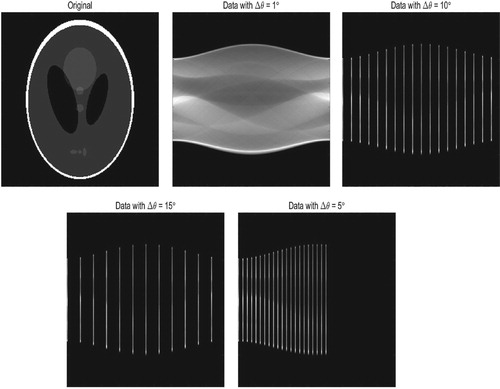
In the following numerical simulations, we consider test problems of modelling the standard 2D parallel-beam tomography. We consider the full-angle model using 180 projection angles evenly distributed between 1 and 180 degrees, in which 367 detector pixels are used. Referring to Figure 1, we show the Shepp-Logan phantom of size $N\times N$ with N=256, the sinogram in the projection space with the angular step size $\mathrm{\Delta }\theta =1^{\circ }$, ${10}^{\circ }$, ${15}^{\circ }$ and the limited angle data consists of 21 projections with total opening angle of ${100}^{\circ }$ ($\mathrm{\Delta }\theta =5^{\circ }$). The Gaussian noise is added to the data $g^{\delta }=g+\epsilon n$ where g denotes the theoretical value of Radon transformation, ϵ is noise level, and $n\sim \mathcal{N}(0,1)$ is a Gaussian random variable.

Figure 1. The original image and the projection data in sinogram form. The angular step size $\mathrm{\Delta }\theta =1^{\circ }$, ${10}^{\circ }$, ${15}^{\circ }$ (the total view angle is ${180}^{\circ }$) respectively and total opening angle is ${100}^{\circ }$, the angular step size $\mathrm{\Delta }\theta =5^{\circ }$. The missing parts of sinograms are denoted by black.

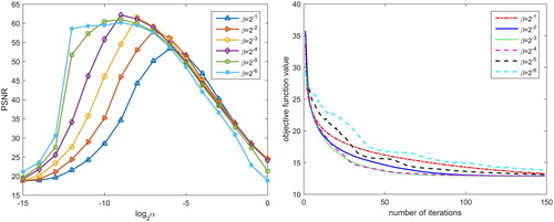
We first analyse the parameters in split Bregman iteration, and give some suggestions about how to choose the parameters. It is observed that there are two parameters α and β in split Bregman iteration. α is the regularization parameter, and β is a Lagrange parameter. In order to test the influence of two parameters on the algorithm, we take $\beta =2^{-l}(l=1,2,\dots ,6)$, and the parameter $\alpha =2^{-j}(j=0,1,2,\dots ,19)$ (i.e. $\alpha \in {\mathrm{\Delta }}_q$ with $q=\frac{1}{2}$). As initial guess, we choose $f_0,d_0,b_0$ to be the zero elements. Iterations are terminated when $\parallel f_k-f_{k-1}\parallel /\parallel f_k\parallel <5\times {10}^{-4}$. The maximal iterative step $K_{max}=400$. We take $\mathrm{\Delta }\theta ={10}^{\circ }$ and $\epsilon =0.01$, and record the numerical results (the PSNR value) for split Bregman iteration with different α and β in Figure 2. Moreover, we fix $\alpha =2^{-7}$, and report the objective functional value for different β. It follows that for the fixed β, α should be chosen appropriately to obtain the higher PSNR value. Figure 2 also shows that β affects the convergence speed. We can have better reconstructed quality and faster convergence speed by choosing $\beta =2^{-3},2^{-4}$, thus we fix $\beta =2^{-3}$ in the following tests.

Figure 2. small The numerical results with split Bregman iteration: the PSNR value and the objective function value when β varies ($\mathrm{\Delta }\theta ={10}^{\circ },\epsilon =0.01$).

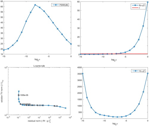
Now we illustrate the performance of the posterior parameter rules: DP rule and heuristic parameter choice rules: the L-curve rule and HR rule. We define $S(\alpha ,g^{\delta }):=\parallel \mathcal{R}{f}_{\alpha }-g^{\delta }\parallel ,H(\alpha ,g^{\delta }):=\frac{\parallel \mathcal{R}{f}_{\alpha }-g^{\delta }{\parallel }^2}{\alpha }.$ In Figure 3, we plot the corresponding results on the value of PSNR, the residual $S(\alpha ,g^{\delta })$, $H(\alpha ,g^{\delta })$ and curve $(\log (\parallel f_{\alpha }{\parallel }_{TV}),\log (\parallel R{f}_{\alpha }-g^{\delta }{\parallel }^2\left)\right)$. It indicates that: (i) the value of PSNR increases first and then decreases after some small α, we can get the optimal regularization parameter α by using manual parameter selection with known original image; (ii) the residual $S(\alpha ,g^{\delta })$ shrinks with the decrease of α, then DP rule can be satisfied with $\tau >1$. However, the noise level δ should be known in advance; (iii) L-curve $(\log (\parallel f_{\alpha }{\parallel }_{TV}),\log (\parallel R{f}_{\alpha }-g^{\delta }{\parallel }^2\left)\right)$ indeed looks like the letter ‘L’, and we can get its corner; (iv) the value of $H(\alpha ,g^{\delta })$ decreases first and then increases, which implies a global minimizer.

Figure 3. The numerical results with split Bregman iteration: the PSNR value, residual $S(\alpha ,g^{\delta })$, $(\log (\parallel f_{\alpha }{\parallel }_{TV}),\log (\parallel R{f}_{\alpha }-g^{\delta }{\parallel }^2\left)\right)$, $H(\alpha ,g^{\delta })$ when $\beta =2^{-3}$, $\mathrm{\Delta }\theta ={10}^{\circ },\epsilon =0.01$.

In order to give the comparison results, we perform the numerical simulations when the regularization parameter α is chosen by manual tuning, DP rule, HR rule and the L-curve rule. We choose ${\alpha }_0=1$, and ${\alpha }_j={\alpha }_0{q}^j$, $j=1,\dots ,40$ with q=0.8. The optimal parameter (RegPara), the PSNR value, the relative errors (RelErr) and the measure of mean structural similarity index (SSIM) under different noise levels are summarized in Table 1. As comparisons we also consider the DP rule with various choices of τ to choose regularization parameters. From Table 1 it can be seen that, for DP rule, the choice of τ influences the accuracy of algorithm. A proper τ should be given, which corresponds to the proper estimation of the noise level. DP rule can give better result if a proper τ is used, however, it can give much worse result if τ is too small or too large. As a special case, when $\delta =1\mathrm{e}-3$, $\tau =1.1$, it gives worse result because it chooses a too small parameter. The L-curve rule and HR rule can give satisfactory reconstruction result although no information on noise level is used. Compared the regularization parameters from the L-curve rule and HR rule with optimal parameters(manual tuning), we notice that the L-curve rule chooses the parameters which are a bit too small and leads to larger errors and HR rule chooses the better parameters which are a little bit more. Because of the ill-posedness of R, a smaller regularization parameter might produce unstable results, which explains that the numerical results by HR rule is superior to that by the L-curve. Figures 4 and 5 show the reconstructed images from the simulated data (the angular step $\mathrm{\Delta }\theta$ be ${10}^{\circ }$, ${15}^{\circ }$) by using split Bregman iteration with different parameter choice rules. Figure 6 shows the results from the limited angle data consisted of 21 projections with total opening angle of ${100}^{\circ }$ ($\mathrm{\Delta }\theta =5^{\circ }$). For enhanced visualization, we also report the difference between the reconstructed image and the original image. We observe that, compared with the manual parameter selection, HR rule produces reasonable results and performs well comparable in terms of visual inspection.

Figure 4. The reconstructed results of SBI (Algorithm 1) with different parameter choice rules: manual parameter selection, DP rule with $\tau =1.1$, the L-curve rule, HR rule. In all cases, the total view angle is ${180}^{\circ }$, the angular step size $\mathrm{\Delta }\theta ={10}^{\circ }$, and $\epsilon =0.01$ (above: reconstruction, below: error map).

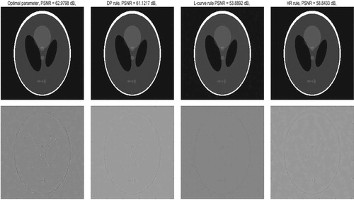
Figure 5. The reconstructed results of SBI (Algorithm 1) with different parameter choice rules: manual parameter selection, DP rule with $\tau =1.1$, the L-curve rule, HR rule. In all cases, the total view angle is ${180}^{\circ }$, the angular step size $\mathrm{\Delta }\theta ={15}^{\circ }$, and $\epsilon =0.01$ (above: reconstruction, below: error map).

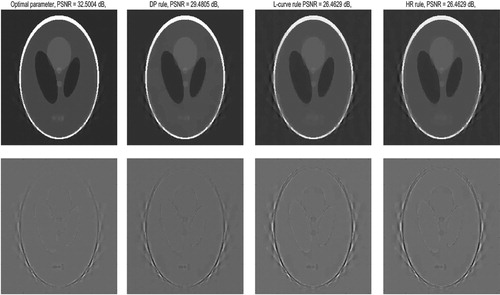
Figure 6. The reconstructed results of SBI (Algorithm 1) with different parameter choice rules: manual parameter selection, DP rule with $\tau =1.1$, the L-curve rule, HR rule. In all cases, The projection data of simulated limited-angle Shepp-Logan phantom (total opening angle is ${100}^{\circ }$, the angular step size $\mathrm{\Delta }\theta =5^{\circ }$ and $\epsilon =0.01$), above: the reconstructed image, below: the error map.

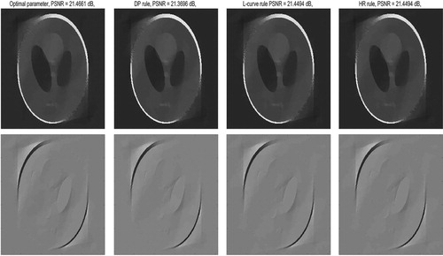
Table 1. Reconstructed results with different noise levels: the value of PSNR, the relative errors (RelErr), SSIM. Regularization parameters(RegPara) are chosen as Manual tuning of the parameters, DP rule, HR rule and the L-curve rule (q=0.8).

ϵ	rule	RegPara	PSNR	RelErr (%)	SSIM
5e−2	Manual tuning	1.44e−02	49.11	1.43	0.9971
	DP rule ($\tau =3$)	1.68e−01	36.74	5.91	0.9716
	DP rule ($\tau =1.1$)	3.52e−02	47.23	1.77	0.9963
	HR rule	4.40e−02	46.15	2.00	0.9954
	L-curve rule	2.42e−03	44.50	2.46	0.9851
1e−2	Manual tuning	2.42e−03	62.98	0.29	0.9998
	DP rule ($\tau =3$)	2.81e−02	51.43	1.09	0.9987
	DP rule ($\tau =1.1$)	5.90e−03	61.12	0.35	0.9972
	HR rule	9.22e−03	58.84	0.46	0.9997
	L-curve rule	7.92e−04	53.89	0.83	0.9994
5e−3	Manual tuning	1.67e−03	67.72	0.17	0.9994
	DP rule ($\tau =3$)	5.90e−03	56.76	1.44	0.9946
	DP rule ($\tau =1.1$)	3.02e−03	66.74	0.19	0.9999
	HR rule	3.02e−03	66.74	0.19	0.9999
	L-curve rule	7.92e−04	56.88	0.59	0.9999
1e−3	Manual tuning	9.90e−04	77.25	0.056	1.0000
	DP rule ($\tau =3$)	1.93e−03	72.24	0.099	1.0000
	DP rule ($\tau =1.1$)	2.08e−04	26.33	20.73	0.7251
	HR rule	9.90e−04	77.25	0.056	1.0000
	L-curve rule	9.90e−04	77.25	0.056	1.0000

In the following, we give some efficient strategies to numerically realize HR rule. It is worth to notice that the whole TV minimization process requires two optimization routines. The outer iteration aims to find a optimal regularization parameter fulfilling HR rule, so a sequence of parameters should be tested. For every test, the inner iteration aims to compute a minimizer of the Tikhonov type functional. In practice, we should give ${\mathrm{\Delta }}_q$, a set of logarithmically spaced regularization parameters and pick the one that minimizes the function H. In this case, if q is too small, then only a very coarse search is performed, and the optimal value is missed. However, if q is close to 1, the test procedure will cost more time. So, from the computational perspective, we give two strategies: (1) we couple TV minimization algorithms with a continuation strategy on the regularization parameter. The reconstructed solution at current parameter is regarded as the initial value of next decreased parameter, and the optimal parameter is chosen by HR rule. This technique of continuation strategy (on the regularization parameter) has been used to the ‘Primal Dual Active Set’ algorithm in [35]. (2) we refine the search by first using a large value of J to identify the best regime for $\{{\alpha }_j{\}}_{j=0,1\dots J}$ by HR rule, then within that regime, using a smaller J (fine searches) to narrow in the best value, and repeating this process until the optimal regularization parameter has been found. Since H function is continuous, this idea is reasonable. In Table 2, we use a small q to choose the regularization parameter, in which ${\alpha }_0$=1e2, ${\alpha }_J=1\mathrm{e}-16$, q=0.1 for the coarse search. We record the numerical results with different noise levels, in which the continuation technique is applied.

Table 2. Reconstructed results with different noise level ($\mathrm{\Delta }\theta ={10}^{\circ }$, q=0.1, $\alpha \in [1\mathrm{e}-16,1\mathrm{e}2]$), Regularization parameter(RegPara) chosen as HR rule, CPU time, the value of PSNR.

ϵ	RegPara	CPU time (s)	PSNR
5e−2	1e−1	695.42	41.02
1e−2	1e−2	701.98	57.83
5e−3	1e−2	690.05	58.77
1e−3	1e−3	698.61	68.36

3.2. Reconstruction of teeth image

In this part, we take an actual clinical CT dicom images (N=512) of teeth as a model, and apply the split Bregman iteration (Algorithm 2 with HR rule) when the projection data with angle increment $\mathrm{\Delta }\theta =5^{\circ }$, ${10}^{\circ }$ respectively.

In the numerical test, we first take q=0.1, ${\alpha }_0=1\mathrm{e}2$, ${\alpha }_J=1\mathrm{e}-16$, and obtain ${\alpha }_{HR}^0=1\mathrm{e}-2$ by Algorithm 2 with HR rule. And then, we determine the interval [1e−1,1e−3] of ${\alpha }_{HR}$ and take q=0.8, ${\alpha }_0=1\mathrm{e}-1$, ${\alpha }_J=1\mathrm{e}-3$ to get the optimal regularization ${\alpha }_{\mathrm{o}\mathrm{p}\mathrm{t}}$. In Table 3, we record the numerical results with the angular step size $\mathrm{\Delta }\theta ={10}^{\circ }$. At the same time, we take the reconstruction of limited data into consideration which consists of 21 projections with total opening angle of ${100}^{\circ }$ ($\mathrm{\Delta }\theta =5^{\circ }$). Note that, when the noise level in real data is unknown, the general discrepancy principle does not work. Observing Figure 7, we can see that the reconstructed results is satisfactory.

Figure 7. The projection data of teeth (the first row): full-angle sinogram with different angular step size $\mathrm{\Delta }\theta =5^{\circ }$, ${10}^{\circ }$ (total view angle is ${180}^{\circ }$) and limited angle sinogram (total opening angle is ${100}^{\circ }$. The reconstructed image and error map of SBI (Algorithm 2) with different parameter choice rules: manual parameter selection (the second row and the third row), HR rule (the fourth row and the fifth row).

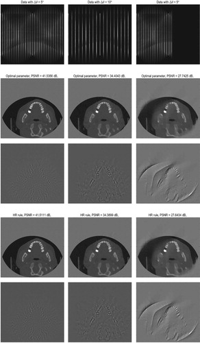
Table 3. Numerical results: The value of PSNR, the relative errors (RelErr), SSIM. Regularization parameter(RegPara) chosen as Manual tuning of the parameters, HR rule with the continuation strategy and without the continuation strategy.

Algorithm	Rule	RegPara	PSNR	RelErr	SSIM
Without continuation	Manual tuning	6.87e−03	34.49	4.80%	0.9450
	HR rule	4.40e−03	34.37	4.86%	0.9460
With continuation	Manual tuning	1.15e−03	34.40	4.84%	0.9450
	HR rule	3.52e−03	34.39	4.85%	0.9447

4. Conclusion

In this paper, as a heuristic parameter choice rule, Hanke Raus rule is introduced to regularization with TV penalty to reconstruct the CT image. Since no a prior noise level is provided in real situations, discrepancy principle is not suitable. Although Hanke Raus rule does not use any information on the noise level, it still gives comparable results.

Compared with the L-curve rule, the Hanke Raus rule has the complete theoretical results even for general penalty term and Banach spaces. From the application's view, for the L-curve rule, there is typical quite a wide range of regularization parameters corresponding to points on the curve near its corner. Moreover, some numerical optimization routines are still needed, like seeking the point on the graph with maximal curvature. While for the Hanke Raus rule, in principle, one could apply a simple optimization algorithm to search automatically. In order to reduce the computational time, we couple TV minimization algorithms with a continuation strategy on the regularization parameter. An important future research problem is to develop more efficient algorithms to numerically realize the Hanke Raus rule.

Acknowledgements

The authors are grateful to the anonymous referees for their useful suggestions and for drawing the authors's attention to relevant references. The authors are grateful to Jin Qinian (Australian National University, Australia) for valuable, helpful comments and discussions.

Disclosure statement

No potential conflict of interest was reported by the authors.

Additional information

Funding

The author Li Li was supported by the National Natural Science Foundation of China (No. 61307023). The author Wang Wei was supported by the National Natural Science Foundation of China (No. 11401257) and Natural Science Foundation of Zhejiang Province (No. LY19A010009).

References

- Natterer F. The mathematics of computerized tomography. Philadelphia (PA): SIAM; 2001.
- Burger M, Müller J, Papoutsellis E, et al. Total variation regularization in measurement and image space for PET reconstruction. Inverse Probl. 2014;30:105003.
- Engl HW, Hanke M, Neubauer A. Regularization of inverse problems. Dordrecht: Kluwer; 1996.
- Schuster T, Kaltenbacher B, Hofmann B, et al. Regularization methods in Banach spaces: radon series on computational and applied mathematics. Berlin: De Gruyter; 2012.
- Guan H, Gordon R. Computed tomography using algebraic reconstruction techniques (ARTs) with different projection access schemes: a comparison study under practical situations. Phys Med Biol. 1996;41:1727–1743. doi: 10.1088/0031-9155/41/9/012
- Xu X, Liow J, Strother SC. Iterative algebraic reconstruction algorithms for emission computed tomography: a unified framework and its application to positron emission tomography. Med Phys. 1993;20:1675–1684. doi: 10.1118/1.596954
- Andersen AH, Kak AC. Simultaneous algebraic reconstruction technique (SART): a superior implementation of the art algorithm. Ultrason Imaging. 1984;6:81–94. doi: 10.1177/016173468400600107
- Kolehmainen V, Lassas M, Siltanen S. Limited data x-ray tomography using nonlinear evolution equations. SIAM J Sci Comput. 2008;30:1413–1429. doi: 10.1137/050622791
- Sidky EY, Pan XC. Image reconstruction in circular cone-beam computed tomography by constrained, total-variation minimization. Phys Med Biol. 2008;53:4777–4807. doi: 10.1088/0031-9155/53/17/021
- Vandeghinste B, Goossens B, Beenhouwer JD, et al. Split-Bregman-based sparse-view CT reconstruction. Fully 3D 2011 proceedings. p. 431–434.
- Chen ZQ, Jin X, Li L, et al. A limited-angle CT reconstruction method based on anisotropic TV minimization. Phys Med Biol. 2013;58:2119–2141. doi: 10.1088/0031-9155/58/7/2119
- Anzengruber SW, Hofmann B, Mathé P. Regularization properties of the sequential discrepancy principle for Tikhonov regularization in Banach spaces. Appl Anal. 2014;93:1382–1400. doi: 10.1080/00036811.2013.833326
- Hansen PC, O'Leary DP. The use of the L-curve in the regularization of discrete ill-posed problems. SIAM J Sci Comput. 1993;14:1487–1503. doi: 10.1137/0914086
- Kindermann S, Neubauer A. On the convergence of the quasioptimality criterion for (iterated) Tikhonov regularization. Inverse Probl Imag. 2008;2:291–299. doi: 10.3934/ipi.2008.2.291
- Hanke M, Raus T. A general heuristic for choosing the regularization parameter in ill-posed problems. SIAM J Sci Comput. 1996;17:956–972. doi: 10.1137/0917062
- Jin B, Lorenz DA. Heuristic parameter-choice rules for convex variational regularization based on error estimates. SIAM J Numer Anal. 2010;48:1208–1229. doi: 10.1137/100784369
- Jin Q. Hanke-Raus heuristic rule for variational regularization in Banach spaces. Inverse Probl. 2016;32:085008.
- Kashef J, Moosmann J, Stotzka R, et al. TV-based conjugate gradient method and discrete L-curve for few-view CT reconstruction of X-ray in vivo data. Opt Express. 2015;23(5):5368–5387. doi: 10.1364/OE.23.005368
- Vogel CR. Non-convergence of the L-curve regularization parameter selection method. Inverse Probl. 1996;12(4):535–547. doi: 10.1088/0266-5611/12/4/013
- Burger M, Osher S. Convergence rates of convex variational regularization. Inverse Probl. 2004;20(5):1411–1421. doi: 10.1088/0266-5611/20/5/005
- Daubechies I, Defrise M, De Mol C. An iterative thresholding algorithm for linear inverse problems with a sparsity constraint. Commun Pur Appl Math. 2004;57:1413–1457. doi: 10.1002/cpa.20042
- Figueiredo MAT, Nowak RD, Wright SJ. Gradient projection for sparse reconstruction: Application to compressed sensing and other inverse problems. IEEE J-STSP. 2008;1:586–597.
- Hale ET, Yin W, Zhang Y. Fixed-point continuation for ℓ1-minimization: methodology and convergence. SIAM J Optim. 2008;19:1107–1130. doi: 10.1137/070698920
- Griesse R, Lorenz DA. A semismooth Newton method for Tikhonov functionals with sparsity constraints. Inverse Probl. 2008;24:035007. doi: 10.1088/0266-5611/24/3/035007
- Jin B, Lorenz D, Schifler S. Elastic-net regularization: error estimates and active set methods. Inverse Probl. 2009;25:1595–1610.
- Beck A, Teboulle M. Fast gradient-based algorithms for constrained total variation image denoising and deblurring problems. IEEE T Image Process. 2009;18:2419–2434. doi: 10.1109/TIP.2009.2028250
- Beck A, Teboulle M. A fast iterative shrinkage-thresholding algorithm for linear inverse problems. SIAM J Imaging Sci. 2009;2:183–202. doi: 10.1137/080716542
- Goldstein T, Osher S. The split Bregman method for ℓ1-regularized problems. SIAM J Imaging Sci. 2009;2:323–343. doi: 10.1137/080725891
- Liu X, Huang L. Split Bregman iteration algorithm for total bounded variation regularization based image deblurring. J Math Anal Appl. 2010;372:486–495. doi: 10.1016/j.jmaa.2010.07.013
- Liu J, Huang TZ, Selesnick IW, et al. Image restoration using total variation with overlapping group sparsity. Inform Sci. 2015;295:232–246. doi: 10.1016/j.ins.2014.10.041
- Sisniega A, Abascal J, Abella M, et al. Iterative Dual-Energy material decomposition for slow kVp switching: a compressed sensing approach. In: XIII Mediterranean Conference on Medical and Biological Engineering and Computing 2013. Cham: Springer; 2014. p. 491–494.
- Nien H, Fessler JA. A convergence proof of the split Bregman method for regularized least-squares problems. Mathematics. arXiv preprint, 2014, arXiv:1402.4371.
- Jiao Y, Jin Q, Lu X, et al. Alternating direction method of multipliers for linear inverse problems. SIAM J Numer Anal. 2016;54:2114–2137. doi: 10.1137/15M1029308
- Wang Z, Bovik AC, Sheikh HR, et al. Image quality assessment: from error visibility to structural similarity. IEEE T Image Process. 2004;13:600–612. doi: 10.1109/TIP.2003.819861
- Fan Q, Jiao Y, Lu X. A primal dual active set algorithm with continuation for continuation for compressed sensing. IEEE T Signal Process. 2014;62:6276–6285. doi: 10.1109/TSP.2014.2362880