Wells' identification and transmissivity estimation in porous media

Abstract

This paper deals with the inverse problems of wells' location and transmissivity estimation in a saturated porous media. Wells are considered as circular holes and the heterogeneous domain is divided into zones with constant transmissivity in each one. The main used tool for wells' location is the topological gradient method applied to a design function defined with respect to available data. Moreover, this technique is incorporated in an adaptive parameterization algorithm leading, in a progressive way, to recover interfaces between hydrogeological zones and transmissivity values. The obtained algorithm allows to recover jointly the transmissivities and the wells' locations. Then the proposed method is tested on a simplified model inspired from the Rocky Mountain aquifer.

Keywords:

• Inverse problem
• topological gradient
• adaptive parameterization
• Wells' location
• transmissivity identification

AMS Subject Classifications:

• 65N20
• 65N21

1. Introduction

Sustainable and resilient management of water resources is a key environmental and socio-economical challenge for this century almost all over the world. The study of a steady flow driven by extraction or injection wells is important for many applications in hydrogeology such as the delineation of protection areas around drinking water wells and/or sources, as required in environmental risk assessment and management/protection/restoration protocols of the water resource.

Indeed, for water supply or/and irrigation, wells are elementary hydraulic structures with major importance because they allow direct access to the water at relatively low cost and/or provide a storage area. Often wells locations are unknown because they are illegal. Localizing them is a crucial step for groundwater management. Wells are modelled either as circular holes in the case their diameter is not negligible with respect to their depth and the domain dimensions or as Dirac functions describing a source term when it is not the case.

Furthermore, inverse modelling is often based on some a priori knowledge of the spatial distribution of model parameters. This a priori data usually include the delineation of zones with constant parameter value (zonation approach) and/or smooth functions (in a geological zone no discontinuities of parameters are expected).

In this work, we consider a heterogeneous saturated porous media containing an unknown number of wells; our goal is recovering both the hydraulic transmissivity distribution and wells' location using available measurements.

The inverse problem of recovering point-sources was studied in the ElectroEncephaloGram (EEG) case by [1–5] for contaminant sources using the advection, dispersive transport equation. In the hydrogeological field in general and for wells in especially, the under-considered problem was investigated in [6,7], where authors use the reciprocity principle to identify the wells' positions. The crucial point of this method is the relevant choice of the test functions and the knowledge of wells' number to be identified. Whereas in [8] the used method is based on the assumption that in the discretized model, each mesh node is considered as a possible point source and the locations of the unknown wells are identified by minimizing a constitutive law gap functional. The main difficulty with the later method, consists in distinguishing neighbouring wells when they are very close.

The topological gradient approach was used to detect geometry defects such as cracks. It is based on geometrical perturbation, was initially introduced by Schumacher [9] in the context of compliance minimization and generalized by Sokolowski and Zochowski [10] with different shape functionals, as done in [11–13]. In the other hand, the adaptive parameterization method founded on refinement indicators firstly introduced in [14,15], is efficient for recovering transmissivity distribution. Yeah [16] also used a finite difference scheme discretization combined with a parametrization of the transmissivities using finite elements and the minimization of kriging errors on head values.

Nevertheless, to our knowledge, there are no references dealing with identification of wells considered as holes inside a heterogeneous domain with unknown transmissivities. So, we propose to combine the topological gradient method to the adaptive parameterization method with refinement indicators in order to identify jointly the transmissivity distribution, considered as a piece-wise constant function, and wells' positions.

This paper is outlined as follows: Section 2 is devoted to define the forward problem. Section 3, deals with the problem of wells' location identification, where the topological asymptotic analysis with geometrical variation is introduced. In Section 4, the principle of the adaptive parameterization method is recalled and then the algorithm combining adaptive parameterization and topological gradient methods is developed. In order to illustrate the efficiency of the proposed algorithms, in each section numerical experiments are presented.

2. Forward problem

A satured horizontal aquifer, confined between impermeable rocks on top and bottom, of constant thickness and isotropic with respect to its hydrogeological parameters is considered. Following [17–19] the groundwater flow is modelled by two-dimensional partial differential equation (1(1) $\begin{array}{l}-\mathrm{div}(T\mathrm{\nabla }{u}_{\epsilon })=0\text{in }\mathrm{\Omega }\mathrm{\setminus }\overline{{\mathcal{O}}_{\epsilon }}\\ u_{\epsilon }=\overline{H}\text{on}{\mathrm{\Gamma }}_1\\ -T\mathrm{\nabla }{u}_{\epsilon }\cdot \mathbf{n}=\overline{\mathrm{\Phi }}\text{on}{\mathrm{\Gamma }}_2\\ u_{\epsilon }=d\text{on }{\mathrm{\Sigma }}_{\epsilon }.\end{array}$(1) ). The domain Ω is divided into sub-domains corresponding to different geological zones. The transmissivity T is a space dependant piecewise constant function [15] supposed to be constant in each zone and discontinuous at the zones' interfaces. This is a standard assumption in groundwater modelling, since no discontinuities of parameter are expected in a geological zone. And even if a parameter is modelled as a smooth function in a geological zone, interpolation allows to come back to identification of constant values; these constant are coefficients of polynomial function.

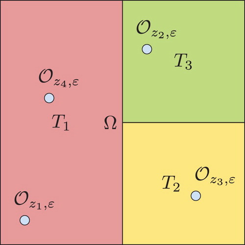
The forward two-dimensional problem of groundwater flow consists in finding the hydraulic head which is equivalent in hydrogeology to the flow velocity. In an isotropic medium, including m circular wells having the same radius ϵ in the domain Ω (Figure 1), this problem can be formulated as follows: (1) $\begin{array}{l}-\mathrm{div}(T\mathrm{\nabla }{u}_{\epsilon })=0\text{in }\mathrm{\Omega }\mathrm{\setminus }\overline{{\mathcal{O}}_{\epsilon }}\\ u_{\epsilon }=\overline{H}\text{on}{\mathrm{\Gamma }}_1\\ -T\mathrm{\nabla }{u}_{\epsilon }\cdot \mathbf{n}=\overline{\mathrm{\Phi }}\text{on}{\mathrm{\Gamma }}_2\\ u_{\epsilon }=d\text{on }{\mathrm{\Sigma }}_{\epsilon }.\end{array}$(1) Where:

• ${\mathcal{O}}_{\epsilon }=\bigcup _{k=1}^m{\mathcal{O}}_{z_k,\epsilon }$ with ${\mathcal{O}}_{z_k,\epsilon }$ a circle of radius ϵ and a centre located at ${\mathbf{z}}_{\mathbf{k}}=(z_{x_k},z_{y_k})$;

• ${\mathrm{\Sigma }}_{\epsilon }=\mathrm{\partial }{\mathcal{O}}_{\epsilon }$ is the wells boundary and ${\mathrm{\Gamma }}_1\cup {\mathrm{\Gamma }}_2$ is the exterior boundary of Ω;

• T is the transmissivity and $u_{\epsilon }$ is the hydraulic head;

• $\overline{H}$ and $\overline{\mathrm{\Phi }}$ are respectively the prescribed hydraulic head and flux;

• $d{\upharpoonright }_{\mathrm{\partial }{\mathcal{O}}_{z_k,\epsilon }}=d_k$ with $d_k$ the Dirichlet condition on the boundary of the well modelled by the hole ${\mathcal{O}}_{z_k,\epsilon }$.

Figure 1. Example of an heterogeneous domain including three geological zones and four wells.

Let's recall that:

• the transmissivity T is the rate of flow under a unit hydraulic gradient through a unit width of aquifer of given saturated thickness.

• and the hydraulic conductivity K is a measure of a material's capacity to transmit water. It is defined as a constant of proportionality relating the specific discharge of a porous medium to the hydraulic gradient.

So, the transmissivity of an aquifer is related to its hydraulic conductivity as follows: T=Kb, with b the aquifer thickness.

According to Dupuit [20], the derivation of well flow equations is based on a basic assumption that the flow is radial in a neighbourhood of the well, and requires the use of analytic formulas for radial flow. These formulas are known in simplified flow situations and the hydraulic head expression around the well is given by Equation (2(2) $\begin{array}{rl}{d}_k& =\frac{{\lambda }_k}{2T\pi }\ln \left(\sqrt{(x-z_{x_k}{)}^2+(y-z_{y_k}{)}^2}\right)\end{array}$(2) ) while the global flow satisfies Equation (3(3) $\begin{array}{rl}{\lambda }_k& ={\int }_{\mathrm{\partial }{\mathcal{O}}_{\epsilon ,k}}{q}_k\mathrm{d}s.\end{array}$(3) ). So, on each well ${\mathcal{O}}_{z_k,\epsilon },1\le k\le m$, the Dirichlet boundary condition is: (2) $\begin{array}{rl}{d}_k& =\frac{{\lambda }_k}{2T\pi }\ln \left(\sqrt{(x-z_{x_k}{)}^2+(y-z_{y_k}{)}^2}\right)\end{array}$(2) (3) $\begin{array}{rl}{\lambda }_k& ={\int }_{\mathrm{\partial }{\mathcal{O}}_{\epsilon ,k}}{q}_k\mathrm{d}s.\end{array}$(3) ${\lambda }_k$ denotes the global flow and $q_k$ the surface flow in the well ${\mathcal{O}}_{z_k,\epsilon }$ [21].

Moreover, wells are considered not close to interfaces separating heterogeneous zones.

Let $\mathrm{\Omega }\mathrm{\setminus }\overline{B(x_0,\epsilon })={\mathrm{\Omega }}_{\epsilon }$, we define the Hilbert spaces: $\begin{array}{rl}{\mathcal{V}}_{\epsilon }& =\{v\in H^1({\mathrm{\Omega }}_{\epsilon }),v=0\text{on}{\mathrm{\Gamma }}_1\}\\ {{\mathcal{V}}_{\epsilon }}^0& =\{v\in {\mathcal{V}}_{\epsilon },v=0\text{on}{\mathrm{\Sigma }}_{\epsilon }\}\end{array}$ According to [22], the weak formulation of (1(1) $\begin{array}{l}-\mathrm{div}(T\mathrm{\nabla }{u}_{\epsilon })=0\text{in }\mathrm{\Omega }\mathrm{\setminus }\overline{{\mathcal{O}}_{\epsilon }}\\ u_{\epsilon }=\overline{H}\text{on}{\mathrm{\Gamma }}_1\\ -T\mathrm{\nabla }{u}_{\epsilon }\cdot \mathbf{n}=\overline{\mathrm{\Phi }}\text{on}{\mathrm{\Gamma }}_2\\ u_{\epsilon }=d\text{on }{\mathrm{\Sigma }}_{\epsilon }.\end{array}$(1) ) can be written as follows: (4) $\begin{array}{l}\text{Find }u\in {{\mathcal{V}}_{\epsilon }}^0\text{ such that:}\\ a(u,w)=l(w),\mathrm{\forall }w\in {{\mathcal{V}}_{\epsilon }}^0\\ \text{where}\\ a(u,w)={\displaystyle {\int }_{\mathrm{\Omega }\mathrm{\setminus }\overline{\mathcal{O}}}T\mathrm{\nabla }v\mathrm{\nabla }w\mathrm{d}x\mathrm{\forall }w\in {{\mathcal{V}}_{\epsilon }}^0}\\ l(w)={\displaystyle {\int }_{{\mathrm{\Gamma }}_2}\overline{\mathrm{\Phi }}w\mathrm{d}s,}\end{array}$(4) where $a(\cdot ,\cdot )$ is a bilinear form continuous and coercive on ${{\mathcal{V}}_{\epsilon }}^0\times {{\mathcal{V}}_{\epsilon }}^0$ and $l(\cdot )$ is a linear form on ${{\mathcal{V}}_{\epsilon }}^0$.

Lax-Milgram theorem provides the existence and the uniqueness of the solution of the direct problem (1(1) $\begin{array}{l}-\mathrm{div}(T\mathrm{\nabla }{u}_{\epsilon })=0\text{in }\mathrm{\Omega }\mathrm{\setminus }\overline{{\mathcal{O}}_{\epsilon }}\\ u_{\epsilon }=\overline{H}\text{on}{\mathrm{\Gamma }}_1\\ -T\mathrm{\nabla }{u}_{\epsilon }\cdot \mathbf{n}=\overline{\mathrm{\Phi }}\text{on}{\mathrm{\Gamma }}_2\\ u_{\epsilon }=d\text{on }{\mathrm{\Sigma }}_{\epsilon }.\end{array}$(1) ).

Let recall that we are interested on a complex inverse problem. It consists: to locate wells, to identify their number, to localize interfaces between the geological zones and to estimate the different transmissivity's values. For this purpose measurements of hydraulic heads inside the domain are used.

In the next section, the problem of well's identification in a homogeneous media by means of topological gradient is studied.

3. Well's identification

In this section a simpler inverse problem is considered; the domain is supposed containing one geological zone with given transmissivity and unknown locations of the wells. In addition, no a priori information on the wells' number is given. Wells' location and implicitly their number are identified, using the topological gradient method.

The idea of this method is to start with a 'safe' domain, without holes, and to study the effect on an objective function, of changing the topology by introducing holes inside the domain [9,23,24]. In the following, a general outlook about the topological gradient method and the main used results is given.

3.1. Topological gradient method

The topological sensitivity analysis has been recognized as an efficient method to solve shape optimization problems. It consists to derive an asymptotic expansion of a shape functional with respect to the size of a small hole created inside the domain. This method was introduced by Schumacher [9] in the context of compliance minimization. Then, Sokolowski and Zochowski [10] generalized it to more general shape functions.

Let Ω be a domain of ${\mathbb{R}}^2$ and $\mathrm{\Gamma }=\mathrm{\partial }\mathrm{\Omega }$. We assume that the distance between the wells ${\mathcal{O}}_{z_k,\epsilon }$ of circular shape, can not be neglected with respect to the dimension of the domain. ${\mathcal{O}}_{z_k,\epsilon }=z_k+\epsilon B^k$, $1\le k\le m$, where ϵ is the common diameter and $B^k\subset {\mathbb{R}}^2$ are bounded and smooth domains containing the origin. The points $z_k\in \mathrm{\Omega }$, $1\le k\le m$, determine the location of the wells (Figure 1). These are the unknowns of the considered inverse problem.

To present the basic idea of this method, let us consider a cost functional $j(\mathrm{\Omega })=J(u_{\mathrm{\Omega }})$ to be minimized, where $u_{\mathrm{\Omega }}$ is the solution to a given PDE (model) defined in Ω. For a small parameter $\epsilon \ge 0$, let $\mathrm{\Omega }\mathrm{\setminus }\overline{B(x_0,\epsilon })={\mathrm{\Omega }}_{\epsilon }$ be the perturbed domain obtained by the creation of a circular hole of radius ϵ around the point $x_0\in \mathrm{\Omega }$. The topological sensitivity analysis provides an asymptotic expansion of j when ϵ goes to zero in the form: (5) $j({\mathrm{\Omega }}_{\epsilon })-j(\mathrm{\Omega })=f(\epsilon )g(x_0)+o(f(\epsilon )).$(5) In this expansion, $f(\epsilon )$ is a positive function going to zero with ϵ. The function g is commonly called topological gradient, or topological derivative. It is usually simple to compute and is obtained using the solution of direct and adjoint problems defined on the initial domain. To minimize the criterion j, one has to create holes at some points x where $g(x)$ is negative.

The topological derivative has been obtained for various problems, arbitrary shaped holes and a large class of shape functionals [13,25–27]. For all $\epsilon >0$, the cost function is defined by : (6) $J_{\epsilon }(u_{\epsilon })={\int }_{{\mathrm{\Omega }}_{\epsilon }}|u_{\epsilon }-d^{\mathrm{obs}}{|}^2\mathrm{d}\mathrm{\Omega },$(6) where $u_{\epsilon }$ is the solution of (1(1) $\begin{array}{l}-\mathrm{div}(T\mathrm{\nabla }{u}_{\epsilon })=0\text{in }\mathrm{\Omega }\mathrm{\setminus }\overline{{\mathcal{O}}_{\epsilon }}\\ u_{\epsilon }=\overline{H}\text{on}{\mathrm{\Gamma }}_1\\ -T\mathrm{\nabla }{u}_{\epsilon }\cdot \mathbf{n}=\overline{\mathrm{\Phi }}\text{on}{\mathrm{\Gamma }}_2\\ u_{\epsilon }=d\text{on }{\mathrm{\Sigma }}_{\epsilon }.\end{array}$(1) ) and $d^{\mathrm{obs}}$ are hydraulic head observations.

Considering the extension by 0 inside the wells ${\mathcal{O}}_{\epsilon }$ we define the injection ${\mathcal{V}}_{\epsilon }^0\hookrightarrow {\mathcal{V}}_0.$ Where ${\mathcal{V}}_0$ is defined on the non-perturbed domain Ω.

$J_0$ denoted the cost function defined on the domain Ω.

The asymptotic expansion of $J_{\epsilon }$ with respect to ϵ is based on Amstutz's work [11]. Let consider the two following hypothesis:

Hypothesis 3.1

For all $\epsilon \ge 0$, it is assumed that there exist a bilinear form ${\tilde{a}}_{\epsilon }$ defined on ${\mathcal{V}}_0\times {\mathcal{V}}_0$ and a linear continuous form ${\tilde{l}}_{\epsilon }$ defined on ${\mathcal{V}}_0$, such that: (7) ${\tilde{a}}_{\epsilon }(w,v_0)={\tilde{l}}_{\epsilon }(v_0)\mathrm{\forall }{v}_0\in {\mathcal{V}}_0.$(7)

Hypothesis 3.2

It is assumed that there exist ${\delta }_a,{\delta }_l,\text{ and }{\delta }_j\in \mathbb{R}$ and a function f defined on ${\mathbb{R}}_{+}$ such that: $\begin{array}{rl}\underset{\epsilon \to 0}{lim}f(\epsilon )& =0\\ ({\tilde{a}}_{\epsilon }-a_0)(u_{\epsilon }^2,v_0)& =f(\epsilon ){\delta }_a+o(f(\epsilon )),\\ ({\tilde{l}}_{\epsilon }-l_0)(v_0)& =f(\epsilon ){\delta }_l+o(f(\epsilon )),\end{array}$ where $v_0$ is the solution of the adjoint problem: (8) $\begin{array}{rl}& a_0(w,v_0)=-D{J}_0(u_0)(w),\mathrm{\forall }w\in {\mathcal{V}}_0.\\ & J_{\epsilon }(u_{\epsilon })-J_0(u_0)=D{J}_0(u_0)(u_{\epsilon }-u_0)+f(\epsilon ){\delta }_J+o(f(\epsilon )).\end{array}$(8) Where $D{J}_0$ denotes the differential of $J_0$ with respect to $u_0\in {\mathcal{V}}_0$, supposing that it exists.

Hence the following theorem given in [11]:

Theorem 3.1

For all $\epsilon \ge 0,$ we denote by $j(\epsilon )=J_{\epsilon }({\mathrm{\Omega }}_{\epsilon })$ if $J_{\epsilon }$ satisfies the hypothesis (3.1) and (3.2), then: the asymptotic expansion of $j(\epsilon )$ is given by: (9) $j(\epsilon )-j(0)=\frac{-1}{\log (\epsilon )}[2\pi T{u}_0(x_0)v_0(x_0)]+o\left(\frac{-1}{\log (\epsilon )}\right)$(9) and, ${\delta }_J(x)=2\pi T(x)u_0(x)v_0(x),\mathrm{\forall }x\in \mathrm{\Omega }.$

For numerical tests the methodology is to compute the topological gradient of the considered cost function in all the domain Ω and to locate the points where it is most negative. According to expansion (5(5) $j({\mathrm{\Omega }}_{\epsilon })-j(\mathrm{\Omega })=f(\epsilon )g(x_0)+o(f(\epsilon )).$(5) ), the larger the absolute value of the topological gradient in a point x is, the larger is the decrease of the cost function due to the creation of a hole at this position.

3.2. Numerical results

To compare the computed positions with the exact ones a relative error ${ϵ}_z$, expressed as a percentage, is defined by: (10) ${ϵ}_z=100\cdot \frac{\Vert {\overrightarrow{Oz}}_{ex}-{\overrightarrow{Oz}}_{id}{\Vert }_2}{\Vert {\overrightarrow{Oz}}_{ex}{\Vert }_2},$(10) where O denotes the origin of the Cartesian coordinate system, it is the left bottom point of the rectangular defining the domain. Subscripts ex and id denote, respectively, exact and identified values.

Numerical trials are performed on a homogeneous rectangular domain of $\mathrm{20,000}\mathrm{m}\times \mathrm{10,000}\mathrm{m}$, the transmissivity of the medium is $T=0.001{\mathrm{m}}^2{\mathrm{s}}^{-1}$. ${\mathrm{\Gamma }}_N$ is composed by the vertical boundaries which are considered impermeable ($\overline{\mathrm{\Phi }}=0$), the Dirichlet condition $\overline{H}=40\mathrm{m}$ is fixed on the upper horizontal boundary (${\mathrm{\Gamma }}_D$) and the measurement data on the lower horizontal boundary (${\mathrm{\Gamma }}_m$) is $H=90\mathrm{m}$. Different cases were studied and commented hereafter:

3.2.1. Sensitivity to the number of measurements

In this section, the behaviour of Algorithm 1 to identify a well located at $z=(6000\mathrm{m},6000\mathrm{m})$ considering different number of hydraulic head's observations inside the domain Ω, is investigated. Note that used measurements are synthetic data resulting from the numerical resolution of a forward problem.

We start by considering full measurements: a measurement at every mesh node ($100\mathrm{\%}$ of data), then consider more realistic situations where only partial measurements of hydraulic head are available. In a first test we reduce the number of measurement by taking one observation in every other node ($50\mathrm{\%}$ of data), then in a second test we consider one observation in every fourth node ($25\mathrm{\%}$ of data) and in the last test one observation in every fifth node is available ($20\mathrm{\%}$ of data).

The results and the corresponding relative errors are summarized in Table 1. As expected the error increases when decreasing the number of measurements, however until $25\mathrm{\%}$ measurements the well's localization is acceptable since the relative error is less than $5\mathrm{\%}$.

Table 1. Well's location and corresponding errors for different number of measurements (case of a well located at $z_{ex}=(6000,6000)\mathrm{m}$).

Number of measurements	$100\mathrm{\%}$	$50\mathrm{\%}$	$25\mathrm{\%}$	$20\mathrm{\%}$
$z_{id}(\mathrm{m})$	$(6080,6002)$	$(6000,5800)$	$(6000,6500)$	$(6500,4000)$
${ϵ}_z[\mathrm{\%}]$	0.68	1.65	4.2	10.05

3.2.2. Sensitivity to relative positions

Pumping from a well in a water table aquifer lowers the water table near the well. This area of influence is known as a cone of depression. When wells are relatively close to each other their areas of influence may have interference [19]. In this paragraph the behaviour of Algorithm 1 with respect to distance between identified wells is studied.

For simplicity, we consider a case with only two wells separated by a distance d varying from $12\times {10}^3\mathrm{m}$ to $2\times {10}^3\mathrm{m}$. Table 2 shows relative errors obtained by Algorithm 1 for four different couple of locations. As expected, one can observe in Table 2 that if the wells are well separated (enough far from each other), the relative errors remain within $10\mathrm{\%}$, whereas when the distance between the wells decreases significantly (less than $4\times {10}^3\mathrm{m}$), the identification becomes less accurate since relative errors increase and are larger than $10\mathrm{\%}$.

Table 2. Relative errors in the case of 2 wells separated by different distances.

Distance $({10}^3\mathrm{m})$	12	8	4	2
${ϵ}_z[\mathrm{\%}]$	1.2	5.22	9.5	10.05

3.2.3. Case of multiple wells

In this test a domain including four wells is considered and Algorithm 1 is applied to recover their locations. Figure 2(a) shows the topological gradient distribution obtained and Figure 2(b) represents exact positions of wells and positions obtained with Algorithm 1. We remark that the recovered locations are close to the exact ones. This remark is confirmed in Table 3 where the exact and identified wells' locations are given as well as the computed relative errors which are smaller than $5\mathrm{\%}$.

Figure 2. Wells' location with Algorithm 1 in the case of four wells. (a) Topological gradient distribution and (b) exact and recovered wells' position.

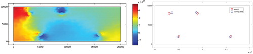
Table 3. Identified locations compared to exact ones in the case of four wells.

$z_{ex}({10}^3\mathrm{m})$	$(5,2$)	$(9,8)$	$(16,2)$	$(3,8)$
$z_{id}({10}^3\mathrm{m})$	$(4.85,1.68)$	$(9.11,8.20)$	$(16.08,2.16)$	$(3.20,8.20)$
${ϵ}_z[\mathrm{\%}]$	4.68	1.78	0.62	3.02

4. Estimate parameters and locate wells jointly

In this section an algorithm combining the topological sensitivity approach and the adaptive parameterization technique [14,15] to locate the positions of a known number of wells, the interface between the different geological zones and to estimate the values of the constant transmissivities in each zone, is developed.

4.1. The adaptive parameterization

In hydrogeology identifying the parameterization is a crucial point in the study of the domain. Because measurements are expensive the main difficulty to solve an inverse problem of parameter estimation in hydrogeology, as well as for many other physical problems, is the lack of data. The idea of the adaptive parameterization method is to reduce the number of unknowns by discretising the considered parameter independently from the discretization of the direct problem. ${\mathcal{T}}_h$ denotes the computing mesh and $\mathcal{Z}$ the zonation. The degrees of freedom of the transmissivity to be estimated are the values of the transmissivity in each zone of $\mathcal{Z}$. 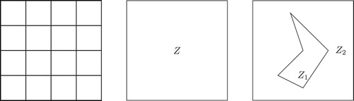The number of zones have to be significantly lower than the number of elements in the computing mesh. The parameterization composed by the zonation and the values of the parameter in each zone, is built iteratively; starting from a homogeneous domain with one geological zone, at each iteration we split only one zone into two zones (see Figure 3). The choice of the zone to refine and the splitting curve is lead by a refinement indicator [15], so the refinement of the parametrization is not arbitrary and not uniform. The new zone is added where the refinement indicators indicate that it should induce a significant decrease of the considered cost function.

Figure 3. An example of parameterization refinement. (a) Computing mesh ${\mathcal{T}}_h$ (b) Zonation associated to ${\mathcal{P}}_1$ and (c) Zonation associated to ${\mathcal{P}}_2$.

4.1.1. Refinement indicators [15]

Let $({\mathcal{P}}_1)$ be an initial problem where the hydraulic transmissivity is constant in all the domain (Figure 3(b)). So we have only one value of the transmissivity to estimate, which is done by minimizing an objective function J with respect to this single variable. $({\mathcal{P}}_2)$ is the parameter estimation problem corresponding to a tentative partition of Ω into two zones $Z_1$ and $Z_2$ having different transmissivities (Figure 3(c)). $T^{\ast }=(T_1^{\ast },T_2^{\ast })$ is the solution of $({\mathcal{P}}_2)$ obtained by minimizing the objective function with respect to the corresponding two variables. If the discontinuity $D=T_1^{\ast }-T_2^{\ast }$ were known, then the solution of minimizing J under the constraint $T_1-T_2=D$ is necessarily $T^{\ast }=(T_1^{\ast },T_2^{\ast })$, the solution of $({\mathcal{P}}_2)$ and for D=0 the $T=(T_0^{\ast },T_0^{\ast })$ solution of the constrained problem is obviously the solution of $({\mathcal{P}}_1)$.

The problem of minimizing the objective function under these constraints written in an algebraic form AT=D, where A is a matrix defining the discontinuities, is $J(T^{\ast })=\underset{AT=D}{min}J(T).$ To this problem we associate the Lagrangian function defined by (11) ${\mathcal{L}}_D(T,\lambda )=J(T)-⟨\lambda ,AT-D⟩,$(11) where λ is the Lagrange multiplier associated to the constraint.

If $J_D^{\ast }=J(T^{\ast })={\mathcal{L}}_D(T^{\ast },{\lambda }^{\ast })$ is the optimal cost associated to the right-hand side D of the constraint, it is deduced from (11(11) ${\mathcal{L}}_D(T,\lambda )=J(T)-⟨\lambda ,AT-D⟩,$(11) ), that (12) $\frac{\mathrm{\partial }{J}_D^{\ast }}{\mathrm{\partial }D}{|}_{D=0}=\frac{\mathrm{\partial }\mathcal{L}}{\mathrm{\partial }D}(T^{\ast },{\lambda }^{\ast }){|}_{D=0}={\lambda }^{\ast }.$(12) Such that the first-order development is: $J_D^{\ast }=J_0^{\ast }+{\lambda }^{\ast }(T_1^{\ast }-T_2^{\ast })+\cdots .$ Therefore the Lagrange multiplier, or refinement indicator gives us the sensitivity of the optimal data cost $J_D^{\ast }$ to the perturbation D. Without solving $({\mathcal{P}}_2)$, this indicator, which can be easily deduced from Equation (12(12) $\frac{\mathrm{\partial }{J}_D^{\ast }}{\mathrm{\partial }D}{|}_{D=0}=\frac{\mathrm{\partial }\mathcal{L}}{\mathrm{\partial }D}(T^{\ast },{\lambda }^{\ast }){|}_{D=0}={\lambda }^{\ast }.$(12) ), indicates through its absolute value, if the suggested refinement is likely to induce an important variation of the optimal objective function. In the case of our example, the refinement indicator associated to splitting the single zone of Figure 3(b)) into two zones of Figure 3(c) is : (13) ${\lambda }^{\ast }=\frac{\mathrm{\partial }J}{\mathrm{\partial }{T}_1}(T^{\ast })=-\frac{\mathrm{\partial }J}{\mathrm{\partial }{T}_2}(T^{\ast }),\text{where}T=(T_0^{\ast },T_0^{\ast }).$(13) Such a refinement is defined by introducing a curve called ‘cut’ (the boundary of $Z_2$ in Figure 3(c)). It divides the domain into only two zones of different transmissivities. In this work we suppose that interfaces between zones are carried by the edges of the computational mesh. The refining curves are thus carried by the edges of mesh cells. We restrict the predefined set of candidate curves to vertical and horizontal lines.

4.2. Numerical results

The presented algorithm is obtained by incorporating the topological gradient into the adaptive parameterization algorithm detailed in [15]. At each iteration it proceed in two steps: at the first step wells are located with the current parameterization then at the second step the parameterization is refined considering the current locations of the wells.

The stopping criterion of the algorithm is one of the following conditions :

• The cost function does not decrease during a number of iterations.

• The cost function is close to zero.

• The refinement indicators are close to zero.

The relative error on the estimated values of the transmissivity expressed as a percentage, over N iterations, is defined by: (14) ${ϵ}_T=100\cdot \frac{{(\sum _{i=1}^N(T_{ex}^i-T_{id}^i{)}^2))}^{1/2}}{{(\sum _{i=1}^N(T_{ex}^i{)}^2)}^{1/2}}.$(14) $T_{ex}$ and $T_{id}$ are, respectively, exact and identified transmissivities values.

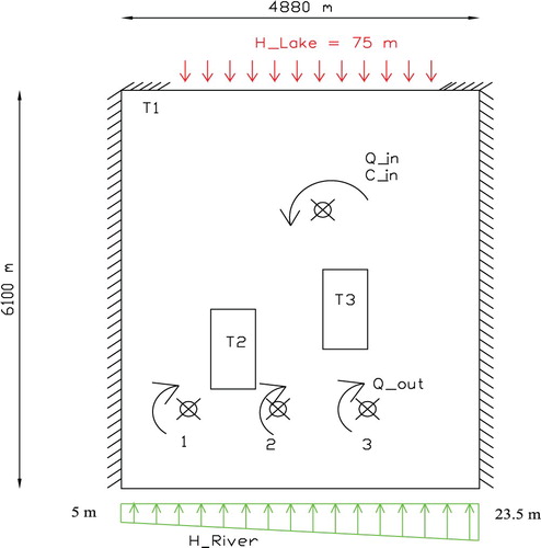
We consider an example inspired from a simplified representation of the Rocky Mountain Arsenal aquifer, Denver, Colorado in USA, based on the detailed model in [28]. It's the simplified idealization studied as a test case in SUTRA code developed by Voss in [29]. This example has the particularity of being composed of three very different transmissivity zones: ranging from ${10}^{-7}{\mathrm{m}}^2/\mathrm{s}$ to ${10}^{-3}{\mathrm{m}}^2/\mathrm{s}$.

This aquifer is supposed to be isotropic and heterogeneous. Figure 4 shows the geometry and boundary conditions data. The domain is $6100\times 4880{\mathrm{m}}^2$ heterogeneous rectangle with a porosity $\omega =0.2$, a constant transmissivity $T_1=2.5\times {10}^{-4}{\mathrm{m}}^2/\mathrm{s}$ and two impermeable bedrock outcrops represented by two rectangles with relative low transmissivities $T_2=T_3=2.5\times {10}^{-7}{\mathrm{m}}^2/\mathrm{s}$. It is bounded by a lake at the north with a constant hydraulic head $h_n=75\mathrm{m}$ and a river at the south with linear hydraulic head, varying from $5\mathrm{m}$ to $23.5\mathrm{m}$ and two impervious lateral borders. The Rocky Mountain aquifer includes three wells (1, 2 and 3) respectively located at ($900\mathrm{m},1200\mathrm{m}$), ($2100\mathrm{m},1200\mathrm{m}$) and ($3300\mathrm{m},1200\mathrm{m}$). A contamination enters the system through a leaking waste isolation pond situated in the north at ($2700\mathrm{m},4200\mathrm{m}$).

Figure 4. Geometry of the Rocky Mountain aquifer.

In [30], authors deal with the same example. They study the identification of the parameterization of both parameters transmissivity and storage coefficient having complete information on the wells.

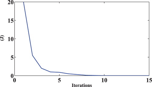
In the following numerical experience data are numerical measurements of the hydraulic head at each node of the computing mesh (full data). The following figures (Figures 5 and 6) show, respectively, the location of the wells and the transmissivities' distribution at different iterations of the Algorithm 2 (iteration 1, 3, 6 for Figure 5 and iteration 12, 15 for Figure 6). The algorithm stops at iteration 15 when the cost function is close to zero; Figure 7 shows the decrease of the cost function during the iterations. We note the convergence towards the sought values of the wells' locations and of the aquifer transmissivities.

Figure 5. Wells' position and parameterization at iterations 1, 3 and 6 with full data.

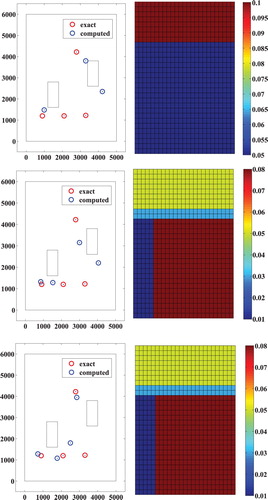
Figure 6. Wells' position and parameterization at iterations 12 and 15 with full data.

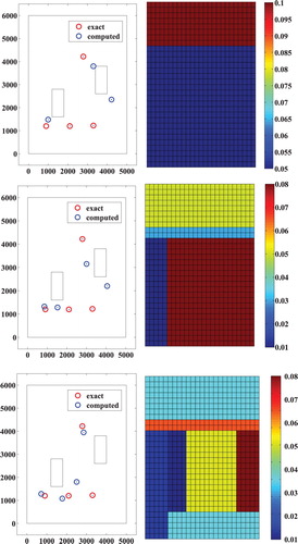
Figure 7. Decrease of the cost function during the iterations in the case of full data (Rocky Mountain example).

4.2.1. Sensitivity to the number of measurements

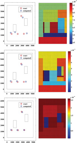
Let's reduce the number of measurements by taking only one measurement in each forth node of the computing mesh. The obtained parametrizations and locations of the wells during different iterations of the Algorithm 2 are presented in Figure 8 and in Figure 9. The algorithm stops at iteration 20 when the cost function is close to zero.

Figure 8. Wells' position and parameterization at iterations 1,3 and 6 with $25\mathrm{\%}$ measurements.

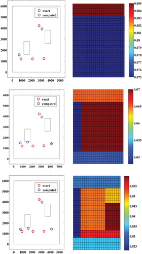
Figure 9. Wells' position and parameterization at iterations 12,15 and 19 with $25\mathrm{\%}$ measurements.

Tables 4 and 5 show the computed locations and corresponding relative errors respectively using full data and $25\mathrm{\%}$ of data. We remark that in the two cases relative errors on the estimated locations of the wells are relatively small (less than $6\mathrm{\%}$).

Table 4. Wells' computed locations and corresponding relative errors using full data (Rocky Mountain example).

Wells	$z_1$	$z_2$	$z_3$	$z_4$
$z_{ex}(\mathrm{m})$	$(900,1200)$	$(2100,1200)$	$(3300,1200)$	$(2700,4200)$
$z_{id}(\mathrm{m})$	$(831,1176)$	$(2106,1199)$	$(3210,1175)$	$(2650,4290)$
${ϵ}_z[\mathrm{\%}]$	4.00	2.14	2.65	0.99

Table 5. Wells' computed locations and corresponding relative errors using $25\mathrm{\%}$ data (Rocky Mountain example).

Wells	$z_1$	$z_2$	$z_3$	$z_4$
$z_{ex}(\mathrm{m})$	$(900,1200)$	$(2100,1200)$	$(3300,1200)$	$(2700,4200)$
$z_{id}(\mathrm{m})$	$(815,1350)$	$(1910,1289)$	$(3398,1190)$	$(2610,4081)$
${ϵ}_z[\mathrm{\%}]$	5.12	4.73	2.53	2.97

For transmissivities' recovering, Tables 6 and 7 present the computed values at different iterations of Algorithm 2, using respectively full data and $25\mathrm{\%}$ of data. On Table 8 the obtained results are summarized and as expected in the first case relative error ($2.46\mathrm{\%}$) is smaller than in the second case ($12.01\mathrm{\%}$).

Table 6. Transmissivities' values at different iterations: Rocky Mountain example with full data.

$T({10}^{-3}{\mathrm{m}}^2/\mathrm{s})$	$T_1$	$T_3$	$T_6$	$T_9$	$T_{12}$	$T_{15}$
iter. 1	9
iter. 3	3.7	7.9
iter. 6	0.9	2.5	5.5
iter. 12	0.25	0.47	0.31	0.25	0.35
iter. 15	0.25	0.249	0.25	0.23	0.25	$2.52\times {10}^{-4}$
$T_{ex}$	0.25	0.25	0.25	0.25	0.25	$2.5\times {10}^{-4}$
${ϵ}_T[\mathrm{\%}]$				2.46

Table 7. Transmissivities' values at different iterations: Rocky Mountain example with $25\mathrm{\%}$ data.

$T({10}^{-3}{\mathrm{m}}^2/\mathrm{s})$	$T_1$	$T_3$	$T_6$	$T_9$	$T_{12}$	$T_{15}$	$T_{19}$
iter. 1	9
iter. 3	5.6	7.9
iter. 6	3.59	4.9	5.51
iter. 12	0.89	0.46	0.35	0.55	0.35
iter. 15	0.39	0.27	0.29	0.23	0.27	$2.1\times {10}^{-3}$
iter. 19	0.259	0.22	0.266	0.231	0.257	0.198	$2.751\times {10}^{-4}$
$T_{ex}$	0.25	0.25	0.25	0.25	0.25	0.25	$2.5\times {10}^{-4}$
${ϵ}_T[\mathrm{\%}]$					12.01

Table 8. Recovered transmissivities and corresponding relative errors with full and reduced data (Rocky Mountain example).

$T({10}^{-3}{\mathrm{m}}^2/\mathrm{s})$	$T_{1ex}$	$T_{1id}^{min}÷T_{1id}^{max}$	$T_{2ex}$	$T_{2id}^{min}÷T_{2id}^{max}$	${ϵ}_T[\mathrm{\%}]$
Full data	0.25	$0.23÷0.258$	$2.5\times {10}^{-4}$	${2.210}^{-4}÷2.52\times {10}^{-4}$	2.46
$25\mathrm{\%}$ data	0.25	$0.198÷0.282$	$2.5\times {10}^{-4}$	${2.1210}^{-4}÷2.75\times {10}^{-4}$	12.01

In conclusion, the relative errors obtained on the transmissivities values as well as those on the wells' location are good taking into account that the number of measurements are relatively small in the second considered case.

4.2.2. Sensitivity to noisy data

In realistic situations, measurements are usually polluted by errors due to measurement devices, technicians handling them, and so on. To study the sensitivity of the Algorithm 2 with respect to noise, a uniform white noise, with zero mean, is applied to the hydraulic head data.

We consider that noised full data is available. Figures 10–12 show wells' location and parameterization at different iterations of Algorithm 2, obtained, respectively, with a noise level of $2\mathrm{\%}$, $4\mathrm{\%}$ and $8\mathrm{\%}$. For tests with noise level of $2\mathrm{\%}$ and $4\mathrm{\%}$, the algorithm stops when the cost function is close to zero. This condition is reached respectively at iteration 21 and 23, while for the test with noise level of $8\mathrm{\%}$, the algorithm stops at iteration 19 when the cost function does not decrease (see Tables 9–11).

Figure 10. Wells' position and parameterization at iterations 12, 15 and 19 with $2\mathrm{\%}$ noise on full data.

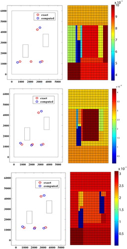
Figure 11. Wells' position and parameterization at iterations 12, 15 and 23 with $4\mathrm{\%}$ noise on full data.

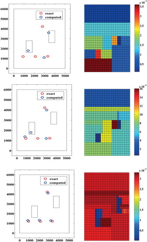
Figure 12. Wells' position and parameterization at iterations 12, 15 and 19 with $8\mathrm{\%}$ noise on full data.

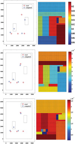
Table 9. Transmissivities' values at different iterations: Rocky Mountain example with $2\mathrm{\%}$ noise level.

$T({10}^{-3}{\mathrm{m}}^2/\mathrm{s})$	$T_1$	$T_3$	$T_6$	$T_9$	$T_{12}$	$T_{15}$	$T_{18}$	$T_{21}$
iter. 1	15.8
iter. 3	10.36	8.7
iter. 6	6.35	5.32	7.31
iter.12	0.84	0.69	0.56	0.55	0.53
iter. 15	0.55	0.36	0.35	0.32	0.37	0.45
iter. 21	0.259	0.202	0.266	0.231	0.257	0.282	0.269	$2.9\times {10}^{-4}$
$T_{ex}$	0.25	0.25	0.25	0.25	0.25	0.25	0.25	$2.5\times {10}^{-4}$
${ϵ}_T[\mathrm{\%}]$					11

Table 10. Transmissivities' values at different iterations: Rocky Mountain example with $4\mathrm{\%}$ noise level.

$T({10}^{-3}{\mathrm{m}}^2/\mathrm{s})$	$T_1$	$T_3$	$T_6$	$T_9$	$T_{12}$	$T_{15}$	$T_{18}$	$T_{23}$
iter. 1	13.4
iter. 3	9.2	8.9
iter. 6	5.3	4.9	0.52
iter.12	0.85	0.56	0.34	0.61	0.44
iter. 15	0.49	0.39	0.26	0.28	0.31	$3.6\times {10}^{-4}$
iter. 18	0.272	0.279	0.259	0.26	0.29	$2.98\times {10}^{-4}$	$2.75\times {10}^{-4}$
iter. 23	0.271	0.268	0.257	0.257	0.284	$2.78\times {10}^{-4}$	$2.69\times {10}^{-4}$	$2.66\times {10}^{-4}$
$T_{ex}$	0.25	0.25	0.25	0.25	0.25	0.25	$2.5\times {10}^{-4}$	$2.5\times {10}^{-4}$
${ϵ}_T[\mathrm{\%}]$					19.6

Table 11. Transmissivities' values at different iterations: Rocky Mountain example with $8\mathrm{\%}$ noise level.

$T({10}^{-3}{\mathrm{m}}^2/\mathrm{s})$	$T_1$	$T_3$	$T_6$	$T_9$	$T_{12}$	$T_{15}$	$T_{19}$
iter. 1	11.2
iter. 3	8.32	7.5
iter. 6	4.69	4.12	6.33
iter. 12	0.89	0.46	0.42	0.46	0.5
iter. 15	0.41	0.3	0.33	0.27	0.2	0.45
iter. 19	0.261	0.241	0.255	0.229	$2.8\times {10}^{-4}$	$2.12\times {10}^{-4}$	0.23
$T_{ex}$	0.25	0.25	0.25	0.25	$2.5\times {10}^{-4}$	$2.5\times {10}^{-4}$	0.25
${ϵ}_T[\mathrm{\%}]$				27

The obtained results for different noise levels are summarized in Tables 12 and 13 which shows respectively the wells' location and the values of the transmissivity. We remark that until $8\mathrm{\%}$ of noise level relative errors are acceptable and identification is reached.

Table 12. Well's locations and corresponding relative errors for different noise levels (Rocky Mountain example).

Noise level	$z_{ex}(\mathrm{m})$	$(900,1200)$	$(2100,1200)$	$(3300,1200)$	$(2700,4200)$
$2\mathrm{\%}$	$z_{id}(\mathrm{m})$	(809, 1319)	(2050, 1140)	(3201, 1150)	(2811, 4308)
	${ϵ}_z(\mathrm{\%})$	3.15	2.81	4	3.1
$4\mathrm{\%}$	$z_{id}(m)$	(850, 1341)	(1945, 1295)	(3101, 1290)	(2760, 3984)
	${ϵ}_z[\mathrm{\%}]$	5.02	3.39	4.35	2.8
$8\mathrm{\%}$	$z_{id}(m)$	(790, 1380)	(2351, 1322)	(3096, 1150)	(2808, 3868)
	${ϵ}_z[\mathrm{\%}])$	6	11.51	5.94	4.27

Table 13. Recovered transmissivities and corresponding relative errors for different noise levels (Rocky Mountain example).

$T({10}^{-3}{\mathrm{m}}^2/\mathrm{s})$	$T_{1ex}$	$T_{1id}^{min}÷T_{1id}^{max}$	$T_{2ex}$	$T_{2id}^{min}÷T_{2id}^{max}$	${ϵ}_T[\mathrm{\%}]$
$2\mathrm{\%}$ noise	0.25	$0.202÷0.282$	$2.5\times {10}^{-4}$	${2.9}^{-4}÷3.6\times {10}^{-4}$	11
$4\mathrm{\%}$ noise	0.25	$0.253÷0.315$	$2.5\times {10}^{-4}$	${2.32}^{-4}÷2.78\times {10}^{-4}$	19.63
$8\mathrm{\%}$ noise	0.25	$0.229÷0.302$	$2.5\times {10}^{-4}$	${2.12}^{-4}÷2.8\times {10}^{-4}$	27

Remark

However, we note that with high noise levels ($10\mathrm{\%}$, $20\mathrm{\%}$ and $30\mathrm{\%}$) the presented algorithm does not converge and neither the position of the wells nor the transmissivity distribution are identified. This fact is normal, since we do not introduce regularization methods in the developed approach we do not expect good results with high noise levels. Indeed, without regularization and without further information, errors between the exact and noisy solution of such inverse problem can be arbitrarily large.

5. Conclusion

In this paper, is developed an algorithm that makes benefits of the advantages of the topological gradient method, which is known to be low cost and efficient for detection of small inclusions, and the adaptive parameterization approach, which avoids over parameterization for parameter estimation problem. The main contribution of this work is the incorporation of these two existing independent methods to solve a complex inverse problem in porous media where the unknowns are the parameterization, the values of the transmissivities and the location of wells.

The developed algorithm is appliyed to a simplified model inspired by the Rocky mountain model [28], an often used benchmark example in groundwater community. The obtained results show their potential applicability, especially since the studied domain consists of very different transmissivity zones ranging from ${10}^{-7}{\mathrm{m}}^2/\mathrm{s}$ to ${10}^{-3}{\mathrm{m}}^2/\mathrm{s}$.

Note that in the literature, we find two kind of wells' model: when the diameter of the well is not negligible with respect to its depth and the domain's dimensions then the well can be considered as a circular hole with a radius r; if not wells can be described as point sinks (Dirac functions) [31]. So the topological gradient method can be applied with a geometrical perturbation for the first kind, as done here, or with a source term perturbation for the wells' Dirac representation. Authors are writing a note in which we compare the two methods.

Acknowledgements

The Partenariat Hubert Curien – Utique program is acknowledged for its financial funding through the project indexed 14G1103, as well as the Euro – Mediterranean $3+3$ program through the project 12/MED/03 (Hydrinv).

Disclosure statement

No potential conflict of interest was reported by the authors.

References

- Atmadja J, Bagtzoglou AC. Pollution source identification in heterogeneous porous media. Water Resour Res. 2001;37:2113–2125. doi: 10.1029/2001WR000223
- Atmadja J, Bagtzoglou AC. State of the art report on mathematical methods for groundwater pollution source identification. Environ Forensics. 2001;2:205–214. doi: 10.1006/enfo.2001.0055
- Ben Abda A, Ben Hassen F, Leblond J, et al. Sources recovery from boundary data: a model related to electroencephalography. Math Comput Model. 2009;49:2213–2223. doi: 10.1016/j.mcm.2008.07.016
- Ben Abda A, Mdimagh R, Saada A. Identification of pointwise sources and small size flaw via the reciprocity gap principle; stability estimates. Int J Tomogr Stat. 2006;4.
- Hamdi A. The recovery of a time-dependent point source in a linear transport equation: application to surface water pollution. Inverse Probl. 2009;25:075006.
- Hariga NT, Bouhlila R, Ben Abda A. Identification of aquifer point sources and partial boundary condition from partial overspecified boundary data. Comptes Rendus Geoscience. 2008;340:245–250. doi: 10.1016/j.crte.2007.11.006
- Hariga NT, Bouhlila R, Ben Abda A. Recovering data in groundwater: boundary conditions and wells' positions and fluxes. Comput Geosci. 2011;15:637–645. doi: 10.1007/s10596-011-9231-9
- Mansouri W, Baranger TN, Benameur H, et al. Identification of injection and extraction wells from overspecified boundary data. Inverse Probl Sci Eng. 2017;25:1091–1111. doi: 10.1080/17415977.2016.1222527
- Schumacher A. Topologieoptimierung von Bauteilstrukturen unter Verwendung von Lochpositionierungskriterien [Dr.-Thesis]. Universität-GH Siegen; 1996. TIM-Bericht Nr. T09-01.
- Sokolowski J, Zochowski A. On the topological derivative in shape optimization. SIAM J Control Optim. 1999;37:1251–1272. doi: 10.1137/S0363012997323230
- Amstutz S. The topological asymptotic for Navier Stokes equations. ESAIM Control Optim Cal Var. 2005;11:401–425. doi: 10.1051/cocv:2005012
- Bonnet M, Guzina B. Sounding of finite solid bodies by way of topological derivative. Int J Numer Methods Eng. 2004;61:2344–2373. doi: 10.1002/nme.1153
- Garreau S, Guillaume Ph, Masmoudi M. The topological asymptotic for pde systems the elasticity case. SIAM J Cont Optim. 2001;39:1756–1778. doi: 10.1137/S0363012900369538
- Benameur H, Chavent G, Clèment F, et al. The multi-dimensional refinement indicators algorithm for optimal parameterization. Inverse Ill Posed Probl. 2008;16:107–126.
- Benameur H, Chavent G, Jaffré J. Refinement and coarsening indicators for adaptive parameterization application to the estimation of hydraulic transmissivities. Inverse Probl. 2002;18:775–797. doi: 10.1088/0266-5611/18/3/317
- Yeah WG. Review of parameter identification procedures in groundwater hydrology: the inverse problem. Water Resour Res. 1986;22:95–108. doi: 10.1029/WR022i002p00095
- Bear J. Hydraulics of groundwater; Sections 5 and 8. New York: McGraw-Hill; 1979. 563 pages. ISBN 0070041709.
- De Marsily G. Hydrogèologie quantitative; Section 7. Paris: Masson; 1981. 215 pages. ISBN 2225755.
- Freeze A, Cherry JA. Groundwater; Section 6. Upper Saddle River (NJ): Prentice Hall; 1979. 604 pages.
- Dupuit J. Mouvement de l'eau à travers les terrains permèables. R Hebd Seances Acad Sci. 1857;45:92–96.
- De Marsily G. Quantitative hydrogeology: groundwater hydrology for engineers; Section 7. New-York: Academic Press; 1986. ISBN 0122089162.
- Zienkiewicz OC, Taylor RL, Zhu JZ. The finite element method: its basis and fundamentals; Section 3. 7th ed. 2013. 708 pages. Available from: https://doi.org/10.1016/C2009-0-24909-9. ISBN 978-1-85617-633-0.
- Maatoug H, Masmoudi M. The topological sensitivity analysis for the Quasi-Stokes problem. ESAIM. 2004;10:478–504.
- Masmoudi M, Pommier J, Samet B. The topological asymptotic expansion for the Maxwell equations and some applications. Inverse Probl. 2005;21:547–564. doi: 10.1088/0266-5611/21/2/008
- Masmoudi M. The topological asymptotic, computational methods for control applications. GAKUTO Internat Ser Math Sci Appl. 2001;16:53–72.
- Novotny AA, Feijoo RA, Padra C, et al. Topological sensitivity analysis. Methods Appl Mech Engine. 2003;192:803–829. doi: 10.1016/S0045-7825(02)00599-6
- Samet B, Amstutz S, Masmoudi M. The topological asymptotic for the Helmholtz equation. SIAM J Control Optim. 2003;42:1523–1544. doi: 10.1137/S0363012902406801
- Konikow L. Modeling chloride movement in the alluvial aquifer at the Rocky Mountain Arsenal. Colorado: 1979. (Technical report water-supply paper, USGS; 2044).
- Voss CI. Sutra a model for saturated-unsaturated, variable-density ground-water flow with solute or energy transport. U.S. Geological Survey, U.S. Department of the Interior; 2003. (Technical report; Report 02-4231).
- Riahi MH, Benameur H, Jaffré J, et al. Refinement indicators for estimating hydrogeologic parameters. Inverse Probl Sci Eng. 2018;27:317–339.
- Slodicka M. Finite elements in modeling of flow in porous media: how to describe wells. Acta Math Univ Comenianae. 1998;67:197–214.