Estimating a pressure dependent thermal conductivity coefficient with applications in food technology

ABSTRACT

In this paper, we introduce a method to estimate a pressure dependent thermal conductivity coefficient arising in a heat diffusion model with applications in food technology. The strong smoothing effect of the corresponding direct problem renders the inverse problem under consideration severely ill-posed. Thus specially tailored methods are necessary in order to obtain a stable solution. Consequently, we model the uncertainty of the conductivity coefficient as a hierarchical Gaussian Markov random field (GMRF) restricted to uniqueness conditions for the solution of the inverse problem established in Fraguela et al. [A uniqueness result for the identification of a time-dependent diffusion coefficient. Inverse Probl. 2013;29(12):125009]. Furthermore, we propose a Single Variable Exchange Metropolis–Hastings algorithm (SVEMH) to sample the corresponding conditional probability distribution of the conductivity coefficient given observations of the temperature. Sensitivity analysis of the direct problem suggests that large integration times are necessary to identify the thermal conductivity coefficient. Numerical evidence indicates that a signal to noise ratio of roughly ${10}^3$ suffices to reliably retrieve the thermal conductivity coefficient.

KEYWORDS:

• Metropolis–Hastings
• food technology
• thermal conductivity coefficient
• Gaussian Markov random field
• hierarchical model

2010 MATHEMATICS SUBJECT CLASSIFICATION:

• 62P30

1. Introduction

In this paper, we introduce a method to estimate a time-dependent thermal conductivity coefficient arising in a heat diffusion model with applications in food technology. Therefore, we are interested in an inverse problem governed by a linear parabolic partial differential equation. Of note, this inverse problem is severely ill-posed and stable solution methods demand special mathematical treatment.

According to Infante et al. [1] ‘…In high-pressure processes, food is treated with mild temperatures and high pressures in order to inactivate enzymes and preserve as many of its organoleptic properties as possible’. Consequently, there are several research efforts to model the dynamics of food preservation processes which rely on high pressures away from thermal equilibrium [1–10]. A related problem is to infer thermal properties of materials associated to food preservation processes given measurements of the temperature, see [11]. Accordingly, some authors (see, for example, [12,13]) identify the thermal conductivity coefficient under the assumption that it depends on the temperature. In [14,15] a temporal dependence of such a coefficient in different contexts is considered. Often, solution uniqueness conditions for the inverse problem are not explicitly given, or depend on the geometry of the spatial domain in the model under consideration. A noteworthy approach to the inverse problem in consideration is based on homogenization methods, see Łydżba et al. [16]. There, authors introduce a new method to estimate the equivalent microstructure of a porous medium such that preserves the thermal conductivity that is equivalent to a real porous material.

In this paper, we deal with the identification of a coefficient of thermal conductivity under the assumption that it depends on the pressure applied inside the processing device being modelled. Furthermore, in this work, known sufficient solution uniqueness conditions are taken into account when designing the data acquisition strategy, e.g. increasing pressure linearly during the data acquisition process renders the thermal conductivity coefficient as a function of time. Of note, results on the structural identifiability of the thermal conductivity coefficient are important towards the solution of the inverse problem, see [17].

On the other hand, inferring a thermal conductivity coefficient from temperature observations is a statistical inference problem. Indeed, it is necessary to model first a forward mapping defined by a well posed problem for a partial differential equation with initial and boundary conditions (e.g. Fraguela et al. [17] give conditions for a mapping from thermal conductivity coefficient to temperature to be well defined). Secondly, we must postulate an observation mapping from state variables to data taking into account a signal to noise ratio. This double tier modelling renders the inverse problem as a statistical inference problem. Related previous work includes boundary heat flux and heat source reconstruction in heat conduction problems using the Bayesian paradigm by Wang and Zabaras [18,19]. More in general, Kaipio and Fox [20] offer a review of results and challenges in the Bayesian solution of heat transfer inverse problems. We remark that inverse heat conduction problems are difficult given the smoothing nature of the diffusion operator, see Isakov [21], giving rise to a situation where careful modelling and a large signal to noise ratio are necessary in order to be able to solve the inverse problem in a practical setting. Of note, thermocouples, which are data acquisition devices in the setting considered here, have a signal to noise ratio of roughly ${10}^3$ within all the working temperature regime.

In this paper, we rely on the Bayesian paradigm to model the prior information about the parameter to be inferred. The rationale is as follows. In the solution of inverse problems defined by partial differential equations, it is of paramount importance to model prior distributions that are informed with theoretical features of the governing differential equation. On the other hand, Zellner [22] shows that if Bayes theorem is regarded as a learning process in the context of information theory, then the amount of input information is preserved into the output information coded in the posterior distribution. Consequently, in this paper, we construct a prior distribution that incorporates Theorem 14 of [17], giving rise to an unimodal posterior distribution.

We analyze the arising posterior probability distribution using a specially tailored variant of the Metropolis–Hastings algorithm. Consequently, we use a general purpose probability transition kernel, that commutes with affine transformations of the parameter space and has no tuning parameters, known as the twalk, see Christen and Fox [23]. A related important problem is the development of approximation methods towards fast and efficient sampling the target distribution that arises in the Bayesian solution of inverse problems. See for example, Constantine et al. [24], Wilcox et al. [25] or Zhang et al. [26].

The paper is organized as follows: In Section 1 we describe the direct problem that defines the forward mapping, as well as all theoretical results necessary to pose the two tier formulation of the inverse problem as a statistical inference problem. In Section 3 we show our results and discuss our findings. Finally, in Section 4 we reflect upon the reaches and limitations of our approach and offer some perspectives, as well as some remarks on an implementation procedure for thermal conductivity coefficient identification.

2. Problem statement

We shall consider the mathematical modelling of a food preserving method based on high pressure processing away from thermal equilibrium, see Infante et al. [1]. The physical system is partially observed, thus it gives rise to an inverse problem where we want to infer a thermal conductivity coefficient given temperature observations. We assume that the thermal conductivity coefficient of the food sample depends on pressure only, e.g. $k=k\left(P\right)$, see [9]. There is a wide range of materials for which the thermal conductivity coefficient is known at atmospheric pressure. However, this coefficient is not well-known when the pressure reaches values as the used ones in high-pressure processes. This lack of information makes it important to identify the values of this coefficient at different pressures. Thus, the overall goal is identifying $k\left(P\right)$ from measurements of the temperature T.

2.1. Direct problem or forward mapping

According to Smith et al. [9], a mathematical model of the high pressure food preserving method under consideration can be cast as an initial and boundary value problem for a parabolic partial differential equation as follows (1) $\begin{array}{rl}& \varrho C_p\frac{\mathrm{\partial }T}{\mathrm{\partial }t}-k\left(P\right(t\left)\right)\mathrm{\Delta }T=\alpha \frac{\mathrm{d}P}{\mathrm{d}t}\left(t\right)T\mathrm{i}\mathrm{n}{B}_R\times (0,t_{\mathrm{f}})\\ & k\left(P\right(t\left)\right)\frac{\mathrm{\partial }T}{\mathrm{\partial }\mathbf{n}}=h\left(T^e\left(t\right)-T\right)\mathrm{o}\mathrm{n}\mathrm{\partial }{B}_R\times (0,t_{\mathrm{f}})\\ & T=T_0\mathrm{o}\mathrm{n}{B}_R\times \left\{0\right\},\end{array}$(1) where $B_R\subset R^2$ is a disk with center $(0,0)$ and radius R>0, and $t_{\mathrm{f}}>0$ is the final time. Other model components are as follows: $\alpha >0$ is the coefficient of thermal expansion, $\varrho >0$ the density and $C_p>0$ the specific heat; $P\in {\mathcal{C}}^1\left(\right[0,t_{\mathrm{f}}\left]\right)$ is the pressure applied to the food sample inside the device at time t; $k\ge k_0>0$ is the thermal conductivity; $T^e$ is the external temperature; $\mathbf{n}$ is the outward unit normal vector at the boundary of $B_R$; h>0 is a heat exchange coefficient and $T_0$ is the initial temperature (assumed to be constant).

Other conditions being equal, problem (1(1) $\begin{array}{rl}& \varrho C_p\frac{\mathrm{\partial }T}{\mathrm{\partial }t}-k\left(P\right(t\left)\right)\mathrm{\Delta }T=\alpha \frac{\mathrm{d}P}{\mathrm{d}t}\left(t\right)T\mathrm{i}\mathrm{n}{B}_R\times (0,t_{\mathrm{f}})\\ & k\left(P\right(t\left)\right)\frac{\mathrm{\partial }T}{\mathrm{\partial }\mathbf{n}}=h\left(T^e\left(t\right)-T\right)\mathrm{o}\mathrm{n}\mathrm{\partial }{B}_R\times (0,t_{\mathrm{f}})\\ & T=T_0\mathrm{o}\mathrm{n}{B}_R\times \left\{0\right\},\end{array}$(1) ) has a unique (classical) radial solution T, and defines a forward mapping (2) $F\left(k\right)=T,$(2) i.e. given a thermal conductivity coefficient k, it is possible to evaluate a unique temperature T. In the context in inverse problems, we care about conditions on Equation (2(2) $F\left(k\right)=T,$(2) ) to render parameter k uniquely identifiable given data T. We shall summarize known uniqueness results for the inverse problem in the next section and use them to pose the inverse problem as a statistical inference problem.

2.2. Inverse problem

The inverse problem that we will consider in the paper is to estimate the thermal conductivity coefficient k given experimental measurements of the temperature T.

Remark 2.1

We will assume that the acquisition of the data has been carried out during an experiment designed in such a way that the food sample has been subjected to a known pressure $P\left(t\right)$ monotonously increasing in time. Thus, since P is an injective function, the problem of identifying $k\left(P\right)$ is equivalent to identifying $k\left(t\right)=k\left(P\right(t\left)\right)$. For this reason, from now on we consider k as a time-dependent function.

Fraguela et al. (see Theorem 14 of [17]) established a context in order to ensure the uniqueness of function k. This context is described in the following result:

Theorem 2.1

Let us consider the problem (1(1) $\begin{array}{rl}& \varrho C_p\frac{\mathrm{\partial }T}{\mathrm{\partial }t}-k\left(P\right(t\left)\right)\mathrm{\Delta }T=\alpha \frac{\mathrm{d}P}{\mathrm{d}t}\left(t\right)T\mathrm{i}\mathrm{n}{B}_R\times (0,t_{\mathrm{f}})\\ & k\left(P\right(t\left)\right)\frac{\mathrm{\partial }T}{\mathrm{\partial }\mathbf{n}}=h\left(T^e\left(t\right)-T\right)\mathrm{o}\mathrm{n}\mathrm{\partial }{B}_R\times (0,t_{\mathrm{f}})\\ & T=T_0\mathrm{o}\mathrm{n}{B}_R\times \left\{0\right\},\end{array}$(1) ) and assume that the following hypotheses hold

1. $T^e\left(t\right)\equiv T_0$ for all $t\in [0,t_{\mathrm{f}}]$.

2. P is a linear function in $[0,t_{\mathrm{f}}]$ with $\left(\mathrm{d}P/\mathrm{d}t\right)\equiv \beta >0$ and $P\left(0\right)$ reaches the atmospheric pressure value (therefore, $k\left(0\right)$ is known).

3. k is a right locally analytic function in $[0,t_{\mathrm{f}})$.

4. ${\int }_0^{t_{\mathrm{f}}}k\left(t\right)\mathrm{d}t\le \varrho C_p\frac{(R-r_0{)}^2}{4}.$

5. (3) $\frac{dk}{\mathrm{d}t}\left(t\right)\le \frac{\alpha \beta }{\varrho C_p}\frac{k\left(t\right)}{e^{\left(\alpha \beta /\varrho C_p\right)t}-1},t\in [0,t_{\mathrm{f}}].$(3)

Then, the values of temperature T at two points, one of them on the boundary of $B_R$ and the other one at distance $r_0$ of the center point of $B_R$, determine uniquely the coefficient k.

Note that hypothesis (H5) means an upper estimate of the logarithmic derivative of k. Then, taking in account the positivity of k, we write (4) $k\left(t\right)=\exp \left(u\right(t\left)\right).$(4) In order to discretize u, we shall use an equidistant grid on interval $[0,t_{\mathrm{f}}]$ $t_j=j\tau ,j=0,1,\dots ,n,n\in \mathbb{N},\tau =\frac{t_{\mathrm{f}}}{n}$ and the finite element basis of piecewise linear functions $\{{\varphi }_i{\}}_{i=0}^n$ on $[t_j,t_{j+1}],i=0,1,\dots ,n-1$ such that ${\varphi }_i\left(t_j\right)={\delta }_{ij}$ (Kronecker delta). We assume that (5) $u\left(t\right)=\sum _{i=0}^n{u}_i{\varphi }_i\left(t\right)$(5) and we want to determine $u_i=u\left(t_i\right)$ for $i\ge 1$ ($u_0=\log \left(k\right(0\left)\right)$ is known).

From (5(5) $u\left(t\right)=\sum _{i=0}^n{u}_i{\varphi }_i\left(t\right)$(5) ), hypothesis (H4) can be discretized as follows (6) $\tau \sum _{i=0}^{n-1}\frac{\exp \left(u_{i+1}\right)-\exp \left(u_i\right)}{u_{i+1}-u_i}\le \varrho C_p\frac{(R-r_0{)}^2}{4}.$(6)

On the other hand, in order to increase the robustness of our approximations, we weaken restriction (H5) posing it in variational form. First, if we write (3(3) $\frac{dk}{\mathrm{d}t}\left(t\right)\le \frac{\alpha \beta }{\varrho C_p}\frac{k\left(t\right)}{e^{\left(\alpha \beta /\varrho C_p\right)t}-1},t\in [0,t_{\mathrm{f}}].$(3) ) in terms of u we have (7) $\frac{\mathrm{d}u}{\mathrm{d}t}\left(t\right)\le f\left(t\right),t\in [0,t_{\mathrm{f}}],$(7) where $f\left(t\right)=\left(\alpha \beta /\varrho C_p\right)\left(1/e^{\left(\alpha \beta /\varrho C_p\right)t}-1\right)$.

Now, multiplying Equation (7(7) $\frac{\mathrm{d}u}{\mathrm{d}t}\left(t\right)\le f\left(t\right),t\in [0,t_{\mathrm{f}}],$(7) ) by ${\varphi }_i\left(t\right),i=1,2,\dots ,n$, integrating by parts and using Simpson's rule to approximate the definite integrals, hypothesis (H5) becomes (8) $\frac{u_{i+1}-u_{i-1}}{2}\le \frac{\tau }{3}\left(f\left(\frac{t_i+t_{i-1}}{2}\right)+f\left(t_i\right)+f\left(\frac{t_{i+1}+t_i}{2}\right)\right),$(8) for $i=1,2,\dots ,n-1$.

Let us introduce the following notation. Let us denote by Q the set of functions u such that the corresponding $k\left(t\right)$ in Equation (4(4) $k\left(t\right)=\exp \left(u\right(t\left)\right).$(4) ) satisfies $k_i\ge k_0,i=1,2,\dots ,n$ and hypotheses (H1)–(H5) hold, i.e. u satisfies Equations (6(6) $\tau \sum _{i=0}^{n-1}\frac{\exp \left(u_{i+1}\right)-\exp \left(u_i\right)}{u_{i+1}-u_i}\le \varrho C_p\frac{(R-r_0{)}^2}{4}.$(6) ) and (8(8) $\frac{u_{i+1}-u_{i-1}}{2}\le \frac{\tau }{3}\left(f\left(\frac{t_i+t_{i-1}}{2}\right)+f\left(t_i\right)+f\left(\frac{t_{i+1}+t_i}{2}\right)\right),$(8) ). In Section 2.3 we shall use the above notation to introduce a two tiered formulation of the inverse problem.

2.3. Statistical inversion

In this Subsection we shall use the optimality property of Bayes formula as a learning process, see Zellner [22], to incorporate hypotheses (H1)–(H5) into our prior model of the thermal conductivity coefficient, which we discretize as Equation (5(5) $u\left(t\right)=\sum _{i=0}^n{u}_i{\varphi }_i\left(t\right)$(5) ). Next, we shall correct the prior model with a likelihood function that depends on both, the forward mapping (2(2) $F\left(k\right)=T,$(2) ) and data. Finally, we propose a variant of the Metropolis–Hastings algorithm to explore the arising posterior distribution.

For the sake of clarity, throughout the current Subsection we shall use bold uppercase letters to denote random variables, while instances of the random variables are denoted as in the direct problem.

Let $\hat{\mathbf{U}}=({\mathbf{U}}_0,\dots ,{\mathbf{U}}_n)$ denote the coefficients in Equation (5(5) $u\left(t\right)=\sum _{i=0}^n{u}_i{\varphi }_i\left(t\right)$(5) ) and ${\mathbf{\Sigma }}_2$ its standard deviation, which we assume is the same for all ${\mathbf{U}}_i$, $i=0,\dots ,n.$

We model the prior probability density of $\mathbf{\Theta }=(\hat{\mathbf{U}},{\mathbf{\Sigma }}_2)$ using a hierarchical strategy as follows (9) ${\pi }_{\mathbf{\Theta }}\left(\theta \right)={\pi }_{\mathbf{\Theta }}(\hat{u},{\sigma }_2)={\pi }_{\hat{\mathbf{U}}|{\mathbf{\Sigma }}_2}\left(\hat{u}|{\sigma }_2\right){\pi }_{{\mathbf{\Sigma }}_2}\left({\sigma }_2\right){\chi }_Q\left(\hat{u}\right),$(9) where we denote $\hat{u}=(u_0,u_1,\dots ,u_n{)}^T$. First, we define the indicator function ${\chi }_Q\left(u\right)=\left\{\begin{array}{ll}1& \mathrm{i}\mathrm{f}u\left(t\right)=\sum _{i=0}^n{u}_i{\varphi }_i\left(t\right)\mathrm{s}\mathrm{a}\mathrm{t}\mathrm{i}\mathrm{s}\mathrm{f}\mathrm{i}\mathrm{e}\mathrm{s}\left(6\right),\left(8\right)\mathrm{a}\mathrm{n}\mathrm{d}{u}_i\ge u_0,\\ 0& \mathrm{o}\mathrm{t}\mathrm{h}\mathrm{e}\mathrm{r}\mathrm{w}\mathrm{i}\mathrm{s}\mathrm{e}.\end{array}\right.$

Next, based in the principle of maximum entropy (POME), see [27], we model the prior distribution of ${\sigma }_2$ using a Gamma distribution with probability density function ${\pi }_{{\mathbf{\Sigma }}_{\mathbf{2}}}\left({\sigma }_2\right)=\frac{1}{\mathrm{\Gamma }\left(a\right)b^a}{\sigma }_2^{a-1}\exp \left(-\frac{{\sigma }_2}{b}\right),$ which is characterized by shape and scale parameters a and b, i.e. $\mathbb{E}\left({\sigma }_2\right)=ab$, $\mathrm{v}\mathrm{a}\mathrm{r}\left({\sigma }_2\right)=a{b}^2$. The rationale is that if we only know that the hyperparameter ${\mathrm{\Sigma }}_2$ has support on the set of non-negative real numbers, then the Gamma distribution is the first option as the least informative prior distribution if we maximize the distribution entropy subject to two conditions prescribing the expected value of ${\mathrm{\Sigma }}_2$ and the expected value of the logarithm of ${\mathrm{\Sigma }}_2$, which is equivalent to prescribing the shape and scale parameters. In the examples below we choose a=b=1 such that the prior distribution is monotonically decreasing.

Now, in order to model ${\pi }_{\hat{\mathbf{U}}|{\mathbf{\Sigma }}_2}\left(\hat{u}|{\sigma }_2\right)$, let us consider the following tridiagonal matrix $\hat{A}\in {\mathbb{R}}^{(n+1)\times (n+1)}$ $\hat{A}=\frac{1}{{\tau }^2}\left(\begin{array}{ccccc}2& -1& & & \\ -1& 2& -1& & \\ & \ddots & \ddots & \ddots & \\ & & -1& 2& -1\\ & & & -1& 2\end{array}\right),$ where $\tau =t_{\mathrm{f}}/n$ as before. Of note, $\hat{A}$ is a symmetric positive definite matrix arising if we discretize the negative Laplacian operator with Dirichlet boundary conditions using centred finite differences. Let us denote $\hat{\mathrm{\Sigma }}={\hat{A}}^{-1}$. Then, according to Bardsley [28], the expression $det(2\pi \hat{\mathrm{\Sigma }}{)}^{-1/2}\exp \left(-\frac{1}{2}{\hat{u}}^T\hat{A}\hat{u}\right)$ defines a Gaussian Markov Random Field (GMRF) with precision matrix $\hat{A}$ (and, covariance matrix $\hat{\mathrm{\Sigma }}$). Moreover, we must condition this GMRF to the fact that the first value $u_0$ is known. Let us consider $(1,n)$–block partition of matrices $\hat{\mathrm{\Sigma }}$ and $\hat{A}$ $\hat{\mathrm{\Sigma }}=\left(\begin{array}{cc}{\hat{\mathrm{\Sigma }}}_{11}& {\hat{\mathrm{\Sigma }}}_{12}\\ {\hat{\mathrm{\Sigma }}}_{21}& {\hat{\mathrm{\Sigma }}}_{22}\end{array}\right),\hat{A}=\left(\begin{array}{cc}\alpha & v^T\\ v& A\end{array}\right).$

Then, our conditional density can be taken as a multivariate normal $N(\mu ,\mathrm{\Sigma })$, where the mean μ is the vector $u_0{\hat{\mathrm{\Sigma }}}_{21}{\hat{\mathrm{\Sigma }}}_{11}^{-1}$ and the covariance matrix Σ is the Schur complement of matrix ${\hat{\mathrm{\Sigma }}}_{22}$ in $\hat{\mathrm{\Sigma }}$, i.e. $\mathrm{\Sigma }={\hat{\mathrm{\Sigma }}}_{22}-{\hat{\mathrm{\Sigma }}}_{21}{\hat{\mathrm{\Sigma }}}_{11}^{-1}{\hat{\mathrm{\Sigma }}}_{12}.$

Now, letting $u=(u_1,\dots ,u_n)$ we are ready to set ${\pi }_{\hat{\mathbf{U}}|{\mathbf{\Sigma }}_2}\left(\hat{u}|{\sigma }_2\right)=\left(h(u,{\sigma }_2)\right)/\left(Z_0\left({\sigma }_2\right)\right)$ where $h(u,{\sigma }_2)=det(2\pi \mathrm{\Sigma }{)}^{-1/2}\exp \left(-\frac{1}{2}(u-\mu {)}^{T}A(u-\mu )\right),$ and $Z_0\left({\sigma }_2\right)$ is some unknown normalization constant.

Therefore, our prior probability density in Equation (9(9) ${\pi }_{\mathbf{\Theta }}\left(\theta \right)={\pi }_{\mathbf{\Theta }}(\hat{u},{\sigma }_2)={\pi }_{\hat{\mathbf{U}}|{\mathbf{\Sigma }}_2}\left(\hat{u}|{\sigma }_2\right){\pi }_{{\mathbf{\Sigma }}_2}\left({\sigma }_2\right){\chi }_Q\left(\hat{u}\right),$(9) ) can be written as (10) ${\pi }_{\mathbf{\Theta }}\left(\theta \right)=\frac{h(u,{\sigma }_2)}{Z_0\left({\sigma }_2\right)}{\pi }_{{\mathbf{\Sigma }}_2}\left({\sigma }_2\right){\chi }_Q\left(u\right).$(10)

Remark 2.2

The single variable exchange variant of the Metropolis–Hastings algorithm described below does not require the knowledge of $Z_0\left({\sigma }_2\right)$ although it depends on ${\sigma }_2$.

Next, we derive a formula to evaluate the likelihood of data T given an instance of the parameter $u=(u_1,\dots ,u_n)$, assuming $u_0=\log \left(k\right(0\left)\right)$ is known. Let us denote $G(u{)}_j=\exp (\sum _{l=0}^n{u}_l{\varphi }_l\left(t_j\right))$. We assume that data satisfies (11) $T_{ij}=F\left(G\right(u{)}_j{)}_i+{\xi }_{ij}$(11) where data $T_{ij}=T(r_i,t_j)$ is a measurement of the temperature at points $r_i$ and times $t_j$, while $F\left(G\right(u{)}_j{)}_i$ is the forward mapping (2(2) $F\left(k\right)=T,$(2) ) acting on a instance u of the parameters, while ${\xi }_{ij}$ is Gaussian noise with mean 0, standard deviation ${\sigma }_1$ and probability distribution ${\xi }_{ij}\sim \mathcal{N}(0,{\sigma }_1^2)$. Under the hypothesis of independence of the ${\xi }_{ij}$, we can approximate the conditional probability distribution ${\pi }_{\mathbf{T}|\mathbf{\Theta }}\left(T|\theta \right)$ of T by the product (12) ${\pi }_{\mathbf{T}|\mathbf{\Theta }}\left(T|\theta \right)=\prod _{i,j}\frac{1}{(\sqrt{2\pi }{\sigma }_1{)}^{2n}}\exp \left(-\frac{1}{2{\sigma }_1^2}{\left(T_{ij}-F{\left(G(u{)}_j\right)}_i\right)}^2\right)$(12)

Likelihood (12(12) ${\pi }_{\mathbf{T}|\mathbf{\Theta }}\left(T|\theta \right)=\prod _{i,j}\frac{1}{(\sqrt{2\pi }{\sigma }_1{)}^{2n}}\exp \left(-\frac{1}{2{\sigma }_1^2}{\left(T_{ij}-F{\left(G(u{)}_j\right)}_i\right)}^2\right)$(12) ) is equivalent to $T_{ij}\sim \mathcal{N}\left(F\right(G(u{)}_j{)}_i,{\sigma }_1^2)$, where the mean of T is the solution of the direct problem. Given the likelihood (12(12) ${\pi }_{\mathbf{T}|\mathbf{\Theta }}\left(T|\theta \right)=\prod _{i,j}\frac{1}{(\sqrt{2\pi }{\sigma }_1{)}^{2n}}\exp \left(-\frac{1}{2{\sigma }_1^2}{\left(T_{ij}-F{\left(G(u{)}_j\right)}_i\right)}^2\right)$(12) ) and the prior distribution (10(10) ${\pi }_{\mathbf{\Theta }}\left(\theta \right)=\frac{h(u,{\sigma }_2)}{Z_0\left({\sigma }_2\right)}{\pi }_{{\mathbf{\Sigma }}_2}\left({\sigma }_2\right){\chi }_Q\left(u\right).$(10) ), we obtain a model of the posterior distribution of Θ given T using Bayes identity (13) ${\pi }_{\mathbf{\Theta }|\mathbf{T}}\left(\theta |T\right)\propto {\pi }_{\mathbf{T}|\mathbf{\Theta }}\left(T|\theta \right){\pi }_{\mathbf{\Theta }}\left(\theta \right).$(13)

Of note, no analytical expressions are available of the posterior distribution (13(13) ${\pi }_{\mathbf{\Theta }|\mathbf{T}}\left(\theta |T\right)\propto {\pi }_{\mathbf{T}|\mathbf{\Theta }}\left(T|\theta \right){\pi }_{\mathbf{\Theta }}\left(\theta \right).$(13) ), hence we resort to sampling with Markov Chain Monte Carlo Methods. This is achieved by means of the Metropolis–Hastings algorithm.

Let us denote by $q\left({\theta }^{\mathrm{\prime }}|\theta \right)$ a proposal for a probability transition kernel (in the numerical examples in Section 3 we shall use the probability transition kernel known as twalk of Christen and Fox [23]). Let us denote ${\theta }_m$ a state in the parameter space and ${\theta }^{\mathrm{\prime }}=(u^{\mathrm{\prime }},{\sigma }_2^{\mathrm{\prime }})$ a sample drawn from the proposed probability transition kernel.

In the standard Metropolis–Hastings algorithm the computation of (14) $min\left\{1,\frac{{\pi }_{\mathbf{\Theta }|\mathbf{T}}\left({\theta }^{\prime }|T\right)q\left({\theta }^{\prime }|{\theta }_m\right)}{{\pi }_{\mathbf{\Theta }|\mathbf{T}}\left({\theta }_m|T\right)q\left({\theta }_m|{\theta }^{\prime }\right)}\right\}$(14) is needed. Of note, quotient in (14(14) $min\left\{1,\frac{{\pi }_{\mathbf{\Theta }|\mathbf{T}}\left({\theta }^{\prime }|T\right)q\left({\theta }^{\prime }|{\theta }_m\right)}{{\pi }_{\mathbf{\Theta }|\mathbf{T}}\left({\theta }_m|T\right)q\left({\theta }_m|{\theta }^{\prime }\right)}\right\}$(14) ) has to be calculated through Equation (10(10) ${\pi }_{\mathbf{\Theta }}\left(\theta \right)=\frac{h(u,{\sigma }_2)}{Z_0\left({\sigma }_2\right)}{\pi }_{{\mathbf{\Sigma }}_2}\left({\sigma }_2\right){\chi }_Q\left(u\right).$(10) ), which involves the unknown normalizing constant $Z_0\left({\sigma }_2\right)$.

In order to circumvent this problem, we modify the Single Variable Exchange algorithm described in Nicholls et al. [29], by means of the unbiased estimator $E=\frac{{\pi }_{\mathbf{\Theta }|\mathbf{T}}\left({\theta }^{\prime }|T\right){\pi }_{\mathbf{U}\mathbf{|}{\mathbf{\Sigma }}_{\mathbf{2}}}\left(x|{\sigma }_2\right)q\left({\theta }^{\prime }|\theta \right)}{{\pi }_{\mathbf{\Theta }|\mathbf{T}}\left(\theta |T\right){\pi }_{\mathbf{U}|{\mathbf{\Sigma }}_2}\left(x|{\sigma }_2^{\prime }\right)q\left(\theta |{\theta }^{\prime }\right)}$ of the ratio in (14(14) $min\left\{1,\frac{{\pi }_{\mathbf{\Theta }|\mathbf{T}}\left({\theta }^{\prime }|T\right)q\left({\theta }^{\prime }|{\theta }_m\right)}{{\pi }_{\mathbf{\Theta }|\mathbf{T}}\left({\theta }_m|T\right)q\left({\theta }_m|{\theta }^{\prime }\right)}\right\}$(14) ). Here $\theta =(u,{\sigma }_2)$ and x denotes a sample drawn from the conditional probability distribution ${\pi }_{\mathbf{U}\mathbf{|}{\mathbf{\Sigma }}_{\mathbf{2}}}(\cdot |{\sigma }_2^{\prime })$. Then, Equations (10(10) ${\pi }_{\mathbf{\Theta }}\left(\theta \right)=\frac{h(u,{\sigma }_2)}{Z_0\left({\sigma }_2\right)}{\pi }_{{\mathbf{\Sigma }}_2}\left({\sigma }_2\right){\chi }_Q\left(u\right).$(10) ) and (13(13) ${\pi }_{\mathbf{\Theta }|\mathbf{T}}\left(\theta |T\right)\propto {\pi }_{\mathbf{T}|\mathbf{\Theta }}\left(T|\theta \right){\pi }_{\mathbf{\Theta }}\left(\theta \right).$(13) ) allow us to write (15) $\begin{array}{rl}E& =\frac{{\pi }_{\mathbf{T}|\mathbf{\Theta }}\left(T|{\theta }^{\prime }\right){\displaystyle \frac{h(u^{\prime },{\sigma }_2^{\prime })}{Z_0\left({\sigma }_2^{\prime }\right)}}{\pi }_{{\mathbf{\Sigma }}_2}\left({\sigma }_2^{\prime }\right){\chi }_Q\left(u^{\prime }\right){\displaystyle \frac{h(x,{\sigma }_2)}{Z_0\left({\sigma }_2\right)}}q\left({\theta }^{\prime }|\theta \right)}{{\pi }_{\mathbf{T}\mathbf{|}\mathbf{\Theta }}\left(T|\theta \right){\displaystyle \frac{h(u,{\sigma }_2)}{Z_0\left({\sigma }_2\right)}}{\pi }_{{\mathbf{\Sigma }}_2}\left({\sigma }_2\right){\chi }_Q\left(u\right){\displaystyle \frac{h(x,{\sigma }_2^{\prime })}{Z_0\left({\sigma }_2^{\prime }\right)}}q\left(\theta |{\theta }^{\prime }\right)}\\ & =\frac{{\pi }_{\mathbf{T}\mathbf{|}\mathbf{\Theta }}\left(T|{\theta }^{\prime }\right)h(u^{\prime },{\sigma }_2^{\prime }){\pi }_{{\mathbf{\Sigma }}_2}\left({\sigma }_2^{\prime }\right){\chi }_Q\left(u^{\prime }\right)h(x,{\sigma }_2)q\left({\theta }^{\prime }|\theta \right)}{{\pi }_{\mathbf{T}\mathbf{|}\mathbf{\Theta }}\left(T|\theta \right)h(u,{\sigma }_2){\pi }_{{\mathbf{\Sigma }}_2}\left({\sigma }_2\right){\chi }_Q\left(u\right)h(x,{\sigma }_2^{\prime })q\left(\theta |{\theta }^{\prime }\right)}.\end{array}$(15)

Note that the unknown normalizing constants $Z_0\left({\sigma }_2\right)$ and $Z_0\left({\sigma }_2^{\prime }\right)$ do not appear in Equation (15(15) $\begin{array}{rl}E& =\frac{{\pi }_{\mathbf{T}|\mathbf{\Theta }}\left(T|{\theta }^{\prime }\right){\displaystyle \frac{h(u^{\prime },{\sigma }_2^{\prime })}{Z_0\left({\sigma }_2^{\prime }\right)}}{\pi }_{{\mathbf{\Sigma }}_2}\left({\sigma }_2^{\prime }\right){\chi }_Q\left(u^{\prime }\right){\displaystyle \frac{h(x,{\sigma }_2)}{Z_0\left({\sigma }_2\right)}}q\left({\theta }^{\prime }|\theta \right)}{{\pi }_{\mathbf{T}\mathbf{|}\mathbf{\Theta }}\left(T|\theta \right){\displaystyle \frac{h(u,{\sigma }_2)}{Z_0\left({\sigma }_2\right)}}{\pi }_{{\mathbf{\Sigma }}_2}\left({\sigma }_2\right){\chi }_Q\left(u\right){\displaystyle \frac{h(x,{\sigma }_2^{\prime })}{Z_0\left({\sigma }_2^{\prime }\right)}}q\left(\theta |{\theta }^{\prime }\right)}\\ & =\frac{{\pi }_{\mathbf{T}\mathbf{|}\mathbf{\Theta }}\left(T|{\theta }^{\prime }\right)h(u^{\prime },{\sigma }_2^{\prime }){\pi }_{{\mathbf{\Sigma }}_2}\left({\sigma }_2^{\prime }\right){\chi }_Q\left(u^{\prime }\right)h(x,{\sigma }_2)q\left({\theta }^{\prime }|\theta \right)}{{\pi }_{\mathbf{T}\mathbf{|}\mathbf{\Theta }}\left(T|\theta \right)h(u,{\sigma }_2){\pi }_{{\mathbf{\Sigma }}_2}\left({\sigma }_2\right){\chi }_Q\left(u\right)h(x,{\sigma }_2^{\prime })q\left(\theta |{\theta }^{\prime }\right)}.\end{array}$(15) ) and the quotient is well defined if $u\in Q$. 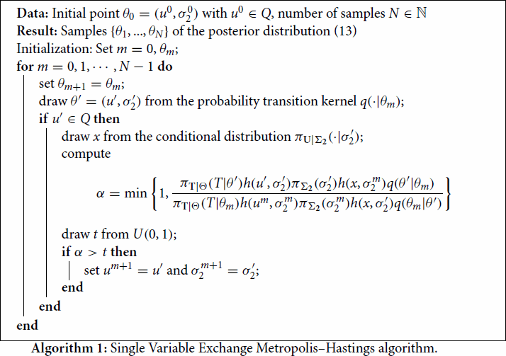This gives rise to Algorithm 1.

Remark 2.3

Algorithm 1 belongs to a wide class of Metropolis–Hastings algorithms with randomized acceptance probability discussed by Nicholls et al. [29], where the ratio of two target distributions is not available (e.g. we do not know the normalizing constant), but can be approximated by an unbiased estimator, e.g. E in Equation (15(15) $\begin{array}{rl}E& =\frac{{\pi }_{\mathbf{T}|\mathbf{\Theta }}\left(T|{\theta }^{\prime }\right){\displaystyle \frac{h(u^{\prime },{\sigma }_2^{\prime })}{Z_0\left({\sigma }_2^{\prime }\right)}}{\pi }_{{\mathbf{\Sigma }}_2}\left({\sigma }_2^{\prime }\right){\chi }_Q\left(u^{\prime }\right){\displaystyle \frac{h(x,{\sigma }_2)}{Z_0\left({\sigma }_2\right)}}q\left({\theta }^{\prime }|\theta \right)}{{\pi }_{\mathbf{T}\mathbf{|}\mathbf{\Theta }}\left(T|\theta \right){\displaystyle \frac{h(u,{\sigma }_2)}{Z_0\left({\sigma }_2\right)}}{\pi }_{{\mathbf{\Sigma }}_2}\left({\sigma }_2\right){\chi }_Q\left(u\right){\displaystyle \frac{h(x,{\sigma }_2^{\prime })}{Z_0\left({\sigma }_2^{\prime }\right)}}q\left(\theta |{\theta }^{\prime }\right)}\\ & =\frac{{\pi }_{\mathbf{T}\mathbf{|}\mathbf{\Theta }}\left(T|{\theta }^{\prime }\right)h(u^{\prime },{\sigma }_2^{\prime }){\pi }_{{\mathbf{\Sigma }}_2}\left({\sigma }_2^{\prime }\right){\chi }_Q\left(u^{\prime }\right)h(x,{\sigma }_2)q\left({\theta }^{\prime }|\theta \right)}{{\pi }_{\mathbf{T}\mathbf{|}\mathbf{\Theta }}\left(T|\theta \right)h(u,{\sigma }_2){\pi }_{{\mathbf{\Sigma }}_2}\left({\sigma }_2\right){\chi }_Q\left(u\right)h(x,{\sigma }_2^{\prime })q\left(\theta |{\theta }^{\prime }\right)}.\end{array}$(15) ).

According to Nicholls et al. [29], the equilibrium distribution of the modified algorithm is the original target distribution.

3. Numerical experiments

In the first part of this Section we explore numerically how the forward mapping propagates uncertainty in the thermal conductivity coefficient. Later, we explore the posterior distribution (13(13) ${\pi }_{\mathbf{\Theta }|\mathbf{T}}\left(\theta |T\right)\propto {\pi }_{\mathbf{T}|\mathbf{\Theta }}\left(T|\theta \right){\pi }_{\mathbf{\Theta }}\left(\theta \right).$(13) ) using Algorithm 1 in three numerical examples. Hypotheses (H1)–(H5) are assumed to hold in all cases. We have used Tylose parameters, a setup of parameter values and dimensions described in Table 1. This parameter set has already been used as a valid synthetic setting in [9]. We have solved the direct problem (1(1) $\begin{array}{rl}& \varrho C_p\frac{\mathrm{\partial }T}{\mathrm{\partial }t}-k\left(P\right(t\left)\right)\mathrm{\Delta }T=\alpha \frac{\mathrm{d}P}{\mathrm{d}t}\left(t\right)T\mathrm{i}\mathrm{n}{B}_R\times (0,t_{\mathrm{f}})\\ & k\left(P\right(t\left)\right)\frac{\mathrm{\partial }T}{\mathrm{\partial }\mathbf{n}}=h\left(T^e\left(t\right)-T\right)\mathrm{o}\mathrm{n}\mathrm{\partial }{B}_R\times (0,t_{\mathrm{f}})\\ & T=T_0\mathrm{o}\mathrm{n}{B}_R\times \left\{0\right\},\end{array}$(1) ) approximating the polar Laplacian and the derivatives in the boundary conditions by means of standard centred order two finite differences and using the classical Crank–Nicolson time stepping, resulting in a second order method, both in time and space. We have discretized the spatial domain with 102 grid points, and we have taken 350 timesteps. Synthetic data sets are created solving the same direct problem with a grid 100 times more fine in time. Observations of temperature at both, the center and a point of the boundary of the ball, are assumed to be polluted with noise according to likelihood (12(12) ${\pi }_{\mathbf{T}|\mathbf{\Theta }}\left(T|\theta \right)=\prod _{i,j}\frac{1}{(\sqrt{2\pi }{\sigma }_1{)}^{2n}}\exp \left(-\frac{1}{2{\sigma }_1^2}{\left(T_{ij}-F{\left(G(u{)}_j\right)}_i\right)}^2\right)$(12) ), where we have chosen the noise standard deviation ${\sigma }_1$ such that the signal to noise ratio (SNR) satisfies (16) $\mathrm{S}\mathrm{N}\mathrm{R}=\frac{\mathrm{m}\mathrm{e}\mathrm{a}\mathrm{n}\left(T\right)}{{\sigma }_1}={10}^3,$(16) and $\mathrm{m}\mathrm{e}\mathrm{a}\mathrm{n}\left(T\right)$ is the mean of the temperature $T=T(r,t)$ for $(t,r)\in B_R\times (0,t_{\mathrm{f}})$ measured in Kelvin degrees. We remark that thermocouples used in real applications to acquire temperature data have roughly the same signal to noise ratio (16(16) $\mathrm{S}\mathrm{N}\mathrm{R}=\frac{\mathrm{m}\mathrm{e}\mathrm{a}\mathrm{n}\left(T\right)}{{\sigma }_1}={10}^3,$(16) ).

Table 1. Parameter setup. We have used parameters and dimensions as described in [9].

Name	Symbol	Value and dimension
Thermal expansion coefficient	α	$4.217\times {10}^{-4}{\mathrm{K}}^{-1}$
Density	ϱ	$1000.6\mathrm{k}\mathrm{g}{\mathrm{m}}^{-3}$
Specific heat	$C_p$	$3780\mathrm{J}{\mathrm{k}\mathrm{g}}^{-1}{\mathrm{K}}^{-1}$
Heat exchange coefficient	h	$28\mathrm{W}{\mathrm{m}}^{-2}{\mathrm{K}}^{-1}$
Inner radius	$r_0$	$0\mathrm{m}$
Outer radius	R	$0.045\mathrm{m}$
Initial temperature	$T_0$	$295\mathrm{K}$
Pressure increase rate	β	$120/61\times {10}^6\mathrm{P}\mathrm{a}{\mathrm{s}}^{-1}$
Final time	$t_{\mathrm{f}}$	$1000\mathrm{s}$

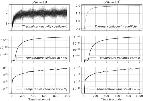
3.1. Sensitivity analysis

Figure 1 illustrates that perturbations in the thermal conductivity coefficient $k=k\left(t\right)$, given by Equation (17(17) $k\left(t\right)=\arctan \frac{t}{30}+\mathrm{0.45.}$(17) ), lead to rather small variance in the corresponding temperature $T=T(r,t)$ at r=0 and r=R. Left column has signal to noise ratio SNR=10 and right column has signal to noise ration $SNR={10}^3$. This feature of the forward mapping (2(2) $F\left(k\right)=T,$(2) ) pinpoints how difficult it is to solve the corresponding inverse problem. Indeed, as Kaipio and Fox [20] establish, such a narrow posterior distribution might give rise to a situation where a computational forward mapping leads to an unfeasible posterior model, e.g. a posterior model such that the true thermal conductivity coefficient has arbitrarily small probability. Of note, Figure 1 also illustrates that the temperature variance is an increasing function of time. Therefore it is possible to design observation times large enough to circumvent the smoothing effect of the forward problem. In the examples shown below we have chosen final time $t_f=1000\mathrm{s}$.

Figure 1. Uncertainty propagation. Subplots in the top row depict 100 perturbed samples of the thermal conductivity coefficient, given by Equation (17(17) $k\left(t\right)=\arctan \frac{t}{30}+\mathrm{0.45.}$(17) ), for $\mathrm{S}\mathrm{N}\mathrm{R}=10$ and $\mathrm{S}\mathrm{N}\mathrm{R}={10}^3$ respectively. Subplots in the middle and the bottom rows depict the variance of the numerical simulation of forward mapping (2(2) $F\left(k\right)=T,$(2) ) acting on the above conductivity coefficients at r=0 and r=R respectively. The smoothing nature of the forward mapping makes it necessary to acquire temperature data at large integration times, e.g. 1000 s.

3.2. Parameter estimation

In each case we have carried out $5\times {10}^5$ steps of the Markov Chain Monte Carlo. In Algorithm 1, we have used the proposal $q\left({\theta }^{\mathrm{\prime }}|\theta \right)$ given by the twalk of Christen and Fox [23]. Our choice was based on the facts that the twalk proposal has no tunning parameters and commutes with affine transformations of space. All programs for the numerical experiments below were coded in python 3.7 and are available in github (https://github.com/MarcosACapistran/diffusion) Following standard notation, we denote by ${\theta }_{\mathrm{M}\mathrm{A}\mathrm{P}}$ the maximum a posteriori probability estimate and by ${\theta }_{CM}$ the conditional mean estimate.

Example 3.1

In the first synthetic example we have used parameters described in Table 1 and thermal conductivity is given by the function (17) $k\left(t\right)=\arctan \frac{t}{30}+\mathrm{0.45.}$(17)

Example 3.2

In the second synthetic example, we have kept the same parameters from Example 3.1, except the thermal conductivity, taking in this case (18) $k\left(t\right)=\frac{1}{2}\left(\arctan \frac{t-450}{150}+3.5\right).$(18)

Example 3.3

Finally, in the third synthetic example the same parameters from previous examples, except the thermal conductivity, are cosidered. In this case we choose (19) $k\left(t\right)=0.4\left({\left(\frac{t}{1000}\right)}^2+\exp \left(-{\left(\frac{t}{1000}\right)}^2\right)\right)+\mathrm{0.05.}$(19)

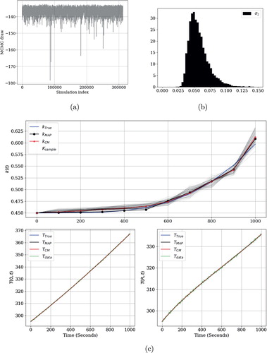
Figures 2,3 and 4 show the results of identifying the thermal conductivity coefficient $k\left(t\right)$ for Examples 3.1, 3.2 and 3.3 respectively. Figures 2(a), 3(a) and 4(a) are numerical evidence of the convergence of the Markov Chain Monte Carlo in the whole of the examples. On the other hand, Figures 2(b), 3(b) and 4(b) show roughly the same marginal posterior distribution for the standard deviation of the prior model for the examples. Of note, the marginal posterior distribution for this hyperparameter has variance smaller than the prior distribution, which we have set equal to 1. Finally, Figures 2(c), 3(c) and 4(c) provide further evidence of the smoothing property of the numerical simulation of the forward mapping (2(2) $F\left(k\right)=T,$(2) ). Although we have used a low dimensional representation (4(4) $k\left(t\right)=\exp \left(u\right(t\left)\right).$(4) ) and (5(5) $u\left(t\right)=\sum _{i=0}^n{u}_i{\varphi }_i\left(t\right)$(5) ) with n=10 in the three cases, it is apparent that the true value of the thermal conductivity coefficient lies in the support of the posterior model.

Figure 2. Example 1. (a) Trace plot. (b) Posterior distribution of ${\sigma }_2$. (c) True and estimators Middle row depicts 2000 samples of the posterior distribution of the thermal conductivity coefficient. At the bottom row are shown the corresponding temperatures evaluated at r=0 and r=R respectively. Hierarchical modelling.

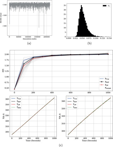
Figure 3. Example 2. (a) Trace plot. (b) Posterior distribution of ${\sigma }_2$. (c) True and estimators Middle row depicts 2000 samples of the posterior distribution of the thermal conductivity coefficient. At the bottom row are shown the corresponding temperatures evaluated at r=0 and r=R respectively. Hierarchical modelling.

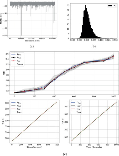
Figure 4. Example 3. (a) Trace plot. (b) Posterior distribution of ${\sigma }_2$. (c) True and estimators Middle row depicts 2000 samples of the posterior distribution of the thermal conductivity coefficient. At the bottom row are shown the corresponding temperatures evaluated at r=0 and r=R respectively. Hierarchical modelling.

In order to explore the accuracy of our method, Table 2 shows the absolute error in the $L^{\mathrm{\infty }}$ norm, between the true solution and the maximum a posteriori estimate, for each example and for $\mathrm{S}\mathrm{N}\mathrm{R}={10}^2,{10}^3$ and ${10}^4$. It is worth highlighting the good accuracy achieved for $\mathrm{S}\mathrm{N}\mathrm{R}={10}^3$, a ratio that, as has been said, is realistic since it is consistent with the margin of error which thermocouples work with. When increasing SNR, the accuracy also increases, but it is a scenario not reachable by the measuring devices. The identification is poorly accurate when a lower SNR is considered, as anticipated by the sensitivity analysis in Section 3.1.

Table 2. Absolute error. We have used ${10}^6$ samples of the MCMC to compute the absolute error $||k-k_{MAP}|{|}_{L^{\mathrm{\infty }}}$ for Examples 3.1, 3.2 and 3.3 at signal to noise ratio (SNR) ${10}^2$, ${10}^3$ and ${10}^4$. Although the MCMC is convergent in every case, a threshold effect is apparent at $\mathrm{S}\mathrm{N}\mathrm{R}={10}^3$.

SNR vs Example	Example 3.1	Example 3.2	Example 3.3
${10}^2$	$9.322234\times {10}^{-1}$	$3.319563\times {10}^{-1}$	$1.061651\times {10}^{-1}$
${10}^3$	$1.599418\times {10}^{-1}$	$1.191929\times {10}^{-1}$	$1.139235\times {10}^{-2}$
${10}^4$	$5.642748\times {10}^{-2}$	$2.620082\times {10}^{-2}$	$2.128011\times {10}^{-3}$

Finally, in order to provide numerical evidence of the efficiency of our algorithm, we present in Table 3 the normalized integrated autocorrelation time (IAT/n) for all the examples and the SNR considered. IAT is a known robust autocorrelation estimator, and normalized by the dimension of the parameter space provides a fair measure of algorithm efficacy.

Table 3. Efficiency. We have used ${10}^6$ samples of the MCMC to compute the measure of effficiency IAT$/n$ for Examples 3.1, 3.2 and 3.3 at signal to noise ratio (SNR) ${10}^2$, ${10}^3$ and ${10}^4$.

SNR	Example 3.1	Example3.2	Example 3.3
${10}^2$	81.5	74.2	95.9
${10}^3$	55.1	39.6	25.8
${10}^4$	29.7	32.9	24.6

4. Conclusions

In this paper we have shown a method to overcome the typical narrowness of the posterior distribution arising in an inverse heat diffusion problem with applications in food technology. Our strategy is to construct a hierarchical prior model of the thermal conductivity coefficient restricted to uniqueness conditions for the solution of the inverse problem. An important feature of our approach is that the variance of the prior model is a parameter to be inferred from data. Finally, we propose a Single Variable Exchange Metropolis–Hastings algorithm to correctly sample the arising posterior distribution. Numerical evidence indicates that the resulting posterior model of the thermal conductivity coefficient contains the true value.

In the numerical implementation, we have resorted to approximation methods to turn the inference of the thermal conductivity coefficient into a parametric problem. We have used a piecewise linear function to approximate the quantity of interest, and inference is carried out over a finite number of real coefficients.

In the context of food technology, the identification algorithm presented here could be applied through the following methodology: The temperature measurements will be acquired through an ad hoc experiment (see Remark 2.1). After that, our algorithm can be applied to identify the thermal conductivity coefficient. Once known its dependence on the pressure for a given food, it can be used for numerical simulation and optimization for high pressure processing of that food.

In the narrative of food technology, the results obtained in this paper might serve as a basis to explore the dimension of the data informed subspace as a function of the signal to noise ratio. The reliable solution of the inverse problem with quantifiable uncertainty provides a basis for industrial analysis towards better controlled food preservation methods.

Acknowledgments

M. A. C. acknowledges partially funding from ONRG, RDECOM and CONACYT CB-2017-284451 grants. J. A. I. R. acknowledges the financial support of the Spanish Ministry of Economy and Competitiveness under the project MTM2015-64865-P and the research group MOMAT (Ref. 910480) supported by Universidad Complutense de Madrid.

Disclosure statement

No potential conflict of interest was reported by the authors.

ORCID

Marcos A. Capistrán  http://orcid.org/0000-0002-7891-6380

Juan Antonio Infante del Río  http://orcid.org/0000-0002-3332-2589

References

- Infante JA, Ivorra B, Ramos AM, et al. On the modelling and simulation of high pressure processes and inactivation of enzymes in food engineering. Math Models Methods Appl Sci. 2009;19(12):2203–2229.
- Adams JB. Enzyme inactivation during heat processing of food-stuffs. Int J Food Sci Technol. 1991;26(1):1–20.
- Cardoso JP, Emery AN. A new model to describe enzyme inactivation. Biotechnol Bioeng. 1978;20(9):1471–1477.
- Hendrickx M, Ludikhuyze L, den Broeck IV, et al. Effects of high pressure on enzymes related to food quality. Trends Food Sci Technol. 1998;9(5):197–203.
- Denys S, Van Loey AM, Hendrickx ME. A modeling approach for evaluating process uniformity during batch high hydrostatic pressure processing: combination of a numerical heat transfer model and enzyme inactivation kinetics. Innovat Food Sci Emerg Technol. 2000;1(1):5–19.
- Otero L, Ramos AM, De Elvira C, et al. A model to design high-pressure processes towards an uniform temperature distribution. J Food Eng. 2007;78(4):1463–1470.
- Norton T, Sun D-W. Recent advances in the use of high pressure as an effective processing technique in the food industry. Food Bioproc Tech. 2008;1(1):2–34.
- Otero L, Guignon B, Aparicio C, et al. Modeling thermophysical properties of food under high pressure. Crit Rev Food Sci Nutr. 2010;50(4):344–368.
- Smith NAS, Mitchell SL, Ramos AM. Analysis and simplification of a mathematical model for high-pressure food processes. Appl Math Comput. 2014;226:20–37.
- Serment-Moreno V, Barbosa-Cánovas G, Torres JA, et al. High-pressure processing: kinetic models for microbial and enzyme inactivation. Food Eng Rev. 2014;6(3):56–88.
- Infante JA, Molina-Rodríguez M, Ramos AM. On the identification of a thermal expansion coefficient. Inverse Probl Sci Eng. 2015;23(8):1405–1424.
- Albu AF, Zubov VI. Identification of thermal conductivity coefficient using a given temperature field. Comput Math Math Phys. 2018;58(10):1585–1599.
- Alifanov OM, Nenarokomov AV, Budnik SA, et al. Identification of thermal properties of materials with applications for spacecraft structures. Inverse Probl Sci Eng. 2004;12(5):579–594.
- Huntul MJ, Lesnic D. An inverse problem of finding the time-dependent thermal conductivity from boundary data. Int Commun Heat Mass Transf. 2017;85:147–154.
- Vabishchevich PN, Klibanov MV. Numerical identification of the leading coefficient of a parabolic equation. Diff Eqs. 2016;52(7):855–862.
- Łydżba D, Różański A, Stefaniuk D. Equivalent microstructure problem: mathematical formulation and numerical solution. Int J Eng Sci. 2018;123:20–35.
- Fraguela A, Infante JA, Ramos AM, et al. A uniqueness result for the identification of a time-dependent diffusion coefficient. Inverse Probl. 2013;29(12):125009.
- Wang J, Zabaras N. A bayesian inference approach to the inverse heat conduction problem. Int J Heat Mass Transf. 2004;47(17-18):3927–3941.
- Wang J, Zabaras N. Hierarchical bayesian models for inverse problems in heat conduction. Inverse Probl. 2004;21(1):183.
- Kaipio JP, Fox C. The bayesian framework for inverse problems in heat transfer. Heat Transf Eng. 2011;32(9):718–753.
- Isakov V. Inverse problems for partial differential equations. Vol. 127. New York: Springer; 2006.
- Zellner A. Optimal information processing and bayes's theorem. Am Stat. 1988;42(4):278–280.
- Christen JA, Fox C. A general purpose sampling algorithm for continuous distributions (the t-walk). Bayesian Anal. 2010;5(2):263–281.
- Constantine PG, Kent C, Bui-Thanh T. Accelerating markov chain monte carlo with active subspaces. SIAM J Sci Comput. 2016;38(5):A2779–A2805.
- Martin J, Wilcox LC, Burstedde C, et al. A stochastic newton MCMC method for large-scale statistical inverse problems with application to seismic inversion. SIAM J Sci Comput. 2012;34(3):A1460–A1487.
- Zhang W, Liu J, Cho C, et al. A fast bayesian approach using adaptive densifying approximation technique accelerated mcmc. Inverse Probl Sci Eng. 2016;24(2):247–264.
- Singh VP, Singh K. Derivation of the gamma distribution by using the principle of maximum entropy (POME) 1. J Am Water Resour Assoc. 1985;21(6):941–952.
- Bardsley JM. Gaussian markov random field priors for inverse problems. Inverse Probl Imaging. 2013;7(2):397–416.
- Nicholls GK, Fox C, Watt AM. Coupled MCMC with a randomized acceptance probability. arXiv preprint arXiv:1205.6857; 2012.