An extended direct factorization method for inverse scattering with limited aperture data

ABSTRACT

In this paper, we propose an extended direct factorization method for solving inverse scattering problems with limited aperture data. It assembles and generalizes two recently developed methods: the extended sampling method and the direct factorization method. With some suitable modification of the direct factorization method, the case with limited aperture data can be effectively handled within the framework of extended sampling method. To further improve the robustness of the original extended sampling method, a novel heuristic iterative algorithm is developed for more accurately estimating the radius of the reconstructed fitting ball which approximately fits the location and size of the unknown scatterer. Moreover, as a major advantage of the direct factorization method, the proposed method does not require any explicit regularization and the knowledge of the noise level in the far-field data. Numerical examples are presented to illustrate the promising efficiency of our proposed method.

KEYWORDS:

• Direct factorization method
• direct sampling method
• extended sampling method
• inverse acoustic scattering
• limited aperture

2010 MATHEMATICS SUBJECT CLASSIFICATIONS:

• 65R32
• 35P25

1. Introduction

Inverse scattering problems [1,2] appear in many fields of science and engineering, such as radar and sonar, biomedical imaging, and non-destructive testing. For solving such nonlinear inverse problems with full aperture data, many efficient and robust numerical algorithms have been developed, see e.g. [3–10]. However, in many real world applications, such as underground mining and underwater submarine detection, only limited aperture data are available and hence the corresponding inverse scattering problem becomes more challenging. This paper is concerned with a new sampling type qualitative method for solving such inverse scattering problems with noisy limited aperture data.

Existing numerical reconstruction algorithms for inverse scattering problems can be roughly categorized into two classes: (i) nonlinear optimization methods, and (ii) qualitative methods. The nonlinear optimization approaches [11–13] often involve an expensive iterative procedure, where a direct (forward) scattering problem needs to be (approximately) solved at each iteration. Although such optimization approaches require less number of incident fields, they do need a priori knowledge of the boundary conditions of the unknown scatterer (e.g. sound-soft or not), and its number of connected components, which may not be available in many practical applications. Furthermore, the optimization iterations may converge to an incorrect approximation of the true scatterer when the provided a priori information (initial guess) is far away from the truth. The qualitative methods [14–17], including the linear sampling method (LSM) [18], the factorization method (FM) [19], direct sampling method (DSM) [9,20], and topological sensitivity method [21–25], have the advantage of not requiring the aforementioned a priori information about the unknown scatterer. Moreover, qualitative methods were shown to be computationally faster than the nonlinear optimization methods, since they determine only an approximation of the scatterer shape and very limited information about its physical/material properties. Our recently proposed direct factorization method (DFM) [26] also belongs to such qualitative methods described above and it was shown to be capable of achieving better reconstruction accuracy than both the regularized FM and the DSM [9]. It is well-known that both LSM and FM also suffer from the severely ill-conditioned discretized far-field operator, which often requires a costly Tikhonov regularization process in order to achieve a robust approximation accuracy in the presence of noise in data. To improve the overall efficiency of the standard FM, the authors [27] recently developed an adaptive quadrature-based factorization method (AFM), which dramatically speeds up the standard FM while produces very reliable and accurate reconstructions. Moreover, the knowledge of the noise level, that is usually required a priori, for the effective implementation of the Tikhonov regularization is not necessary anymore for the case of the newly developed DSM and DFM. Therefore, the regularization-free DSM and DFM are more attractive to real world applications.

All inversion methods discussed above often require a large amount (full aperture) of far-field measurements in order to achieve a satisfactory reconstruction of the shape of the scatterer, which obviously restricts their usefulness in more practical applications. Numerical algorithms for inverse scattering problems with limited aperture data are currently not very widely developed compared to the ones using full aperture. For example see [28–34]. There are also some recent development and generalizations of the above mentioned methods to handle limited aperture data. For example, the approach in [35] only approximately recovers the convex hull of obstacles, while the generalized linear sampling method in [36,37] with carefully chosen penalty regularization terms shows less satisfactory reconstruction quality as the aperture angles get narrower. The DSM indicator function was recently modified in [38] to handle limited observation directions but with full incident directions. In [38], the authors also proposed two data recovery techniques to reconstruct the full aperture far-field data from limited aperture data, and their algorithms were shown to noticeably improve the reconstruction accuracy. To extend the framework of LSM to the case of limited aperture data, an interesting extended sampling method (ESM) was very recently proposed in [39], where the exact far-field pattern of a predefined ball is used to build a new far-field integral equation, with the right-hand-side being the limited aperture noisy far-field data at a fixed incident direction. Based on this new far-field integral equation and some theoretical analysis, an indicator function was computed to identify a ball that provides the approximate support of the scatterer. The ball's radius was estimated through a multilevel procedure which keeps track of the ball centre as the initial guess of the radius is halved along with a refined sampling mesh. A similar far-field integral equation was constructed in the range test method [40], but its main task was to directly obtain a convex support of the scatterer as the intersection of many convex test domains. There is also a short discussion on one possible generalization of the FM to limited aperture data in [19, Section 2.3] via the inf-criterion, but its usefulness was not verified by numerical implementations. In view of the breadth and depth of research works with full aperture data, the more practical problems with limited aperture data are in greater demand, which motivates our current paper.

To summarize, this paper contributes to the generalization and improvement of the original ESM via the DFM framework in terms of the better handling of limited aperture data. In particular, based on our numerical experiments, we found that the current multilevel procedure employed in ESM is not very robust with respect to the initial guess of radius, level of noise and stopping condition. Moreover, all far-field equations are different at each sampling point and hence computational cost is high. In addition, due to ill-conditioness, Tikhonov regularization will further slow down the computation. To address all of these issues, we propose an extended direct factorization method (EDFM), which takes under consideration the advantages of both the ESM and DFM. In particular, the DFM was modified to effectively handle limited aperture data within the framework of ESM. As a significant improvement over the original ESM, a novel iterative algorithm is developed for estimating the radius of the reconstructed ball in a more robust way.

The paper is organized as follows. In Section 2, we provide a brief review of the several related methods (including DFM and DSM) for qualitatively solving inverse acoustic obstacle scattering problems. In Section 3, we formulate and describe the new extended direct factorization method (EDFM). An iterative algorithm for estimating the ball's radius is developed and discussed in detail. In Section 4, a variety of numerical examples with both full and limited aperture data are presented to demonstrate the promising performance of our method. Finally, some conclusions are provided in Section 5.

2. Two recent methods for inverse scattering

Following [1,2], we briefly describe the standard inverse obstacle scattering problem along with two recent numerical methods that are fundamental to build up our proposed method. Let $D\subset {\mathbb{R}}^2$ be a bounded impenetrable sound-soft obstacle with a $C^2$ boundary $\mathrm{\partial }D$. Let θ be an incident direction on the unit circle $\mathbb{S}$ and $\kappa >0$ be the wave number (with wavelength $\lambda =2\pi /\kappa$). Given a time-harmonic incident plane wave field $u^i\left(x\right)=e^{i\kappa x\cdot \theta }$, its propagation in the presence of the obstacle D which is situated in a homogeneous medium will lead to a scattered wave field $u^s$. The obtained total field $u=u^i+u^s$ then solves the following scalar exterior Helmholtz equation (1) $\mathrm{\Delta }u\left(x\right)+{\kappa }^{2}u\left(x\right)=0,x\in {\mathbb{R}}^2\mathrm{\setminus }\overline{D}$(1) subject to the Dirichlet boundary condition (sound-soft) (2) $u=0,\text{on}\mathrm{\partial }D$(2) and the Sommerfeld radiation condition (here $|x|$ denotes the distance between x and the origin) (3) $\underset{|x|\to \mathrm{\infty }}{lim}{|x|}^{1/2}\left(\frac{\mathrm{\partial }{u}^s}{\mathrm{\partial }|x|}-i\kappa u^s\right)=0.$(3) The above direct obstacle scattering problem (1(1) $\mathrm{\Delta }u\left(x\right)+{\kappa }^{2}u\left(x\right)=0,x\in {\mathbb{R}}^2\mathrm{\setminus }\overline{D}$(1) )–(3(3) $\underset{|x|\to \mathrm{\infty }}{lim}{|x|}^{1/2}\left(\frac{\mathrm{\partial }{u}^s}{\mathrm{\partial }|x|}-i\kappa u^s\right)=0.$(3) ) admits a unique solution $u\in C^2\left({\mathbb{R}}^2\mathrm{\setminus }\overline{D}\right)\bigcap C^1\left({\mathbb{R}}^2\mathrm{\setminus }D\right)$. Moreover, the scattered field $u^s$ has an asymptotic behaviour (as $|x|\to \mathrm{\infty }$) $u^s\left(x\right)=\frac{e^{i\kappa |x|}}{{|x|}^{1/2}}{u}_{\mathrm{\infty }}(\hat{x},\theta )+O\left({|x|}^{-3/2}\right)$ uniformly in all directions, where $\hat{x}=x/|x|$ is the observation direction on the unit circle $\mathbb{S}$ and $u_{\mathrm{\infty }}$ is called the far-field pattern. Obviously, the far-field pattern $u_{\mathrm{\infty }}$ depends nonlinearly on the obstacle's shape $\mathrm{\partial }D$.

The standard inverse obstacle scattering problem is then introduced to recover $\mathrm{\partial }D$ from noisy far-field measurement data $u_{\mathrm{\infty }}(\hat{x},\theta )$ with a fixed $\kappa >0$ for all incident $\theta \in {\mathrm{\Gamma }}_s$ and observation directions $\hat{x}\in {\mathrm{\Gamma }}_m$. In the aforementioned discussion of LSM, FM, DSM and DFM, one usually assumes full aperture i.e. ${\mathrm{\Gamma }}_s=[0,2\pi ]$ and ${\mathrm{\Gamma }}_m=[0,2\pi ]$. The case in which ${\mathrm{\Gamma }}_m⊊[0,2\pi ]$ (regardless of the range of ${\mathrm{\Gamma }}_s$), is referred to as the limited aperture data case.

Define the compact far-field integral operator $\mathcal{F}:L^2\left(\mathbb{S}\right)\to L^2\left(\mathbb{S}\right)$ by $\left(\mathcal{F}g\right)\left(\hat{x}\right):={\int }_{\mathbb{S}}{u}_{\mathrm{\infty }}(\hat{x},d)g\left(d\right)\mathrm{d}s\left(d\right).$ Let ${\mathrm{\Phi }}_{\mathrm{\infty }}(\hat{x},z):=\left(e^{i\pi /4}\right)/\left(\sqrt{8\pi \kappa }\right)e^{-i\kappa \hat{x}\cdot z}$ denotes the far-field pattern of the fundamental solution Φ of the Helmholtz equation given by $\mathrm{\Phi }(x,y):=\frac{i}{4}{H}_0^{\left(1\right)}(\kappa |x-y|),x\ne y,$ with $H_0^{\left(1\right)}$ being the Hankel function of the first kind and order zero. The standard LSM and FM are built upon the following linear integral equation (defined for any sampling point $z\in {\mathbb{R}}^2$) $\left(\mathcal{F}{g}_z\right)\left(\hat{x}\right)={\mathrm{\Phi }}_{\mathrm{\infty }}(\hat{x},z),$ and $\left(\right({\mathcal{F}}^{\ast }\mathcal{F}{)}^{1/4}{g}_z\left)\right(\hat{x})={\mathrm{\Phi }}_{\mathrm{\infty }}(\hat{x},z),$ respectively. In general, the FM has more complete mathematical justification than the LSM.

We begin our discussion by defining $2N$ equidistantly distributed angles on the unit circle $\mathbb{S}$: ${\theta }_j=(\cos t_j,\sin t_j),t_j=(j-1)\pi /N,j=1,\dots ,2N.$ Here we naturally extend ${\theta }_j$ as a periodic function of its integer indices: that is ${\theta }_{2N+j}={\theta }_j$ and ${\theta }_{2N-j}={\theta }_{-j}$. We also define a set of incident (source) directions: ${\mathrm{\Gamma }}_s=[{\theta }_{s_1},{\theta }_{s_J}]\mathrm{o}\mathrm{r}\mathrm{i}\mathrm{n}\mathrm{d}\mathrm{i}\mathrm{s}\mathrm{c}\mathrm{r}\mathrm{e}\mathrm{t}\mathrm{e}\mathrm{f}\mathrm{o}\mathrm{r}\mathrm{m}{\mathrm{\Gamma }}_s=\{{\theta }_{s_1},\dots ,{\theta }_{s_j},\dots {\theta }_{s_J}\}$ and a set of observation (measurement) directions: ${\mathrm{\Gamma }}_m=[{\theta }_{m_1},{\theta }_{m_L}]\mathrm{o}\mathrm{r}\mathrm{i}\mathrm{n}\mathrm{d}\mathrm{i}\mathrm{s}\mathrm{c}\mathrm{r}\mathrm{e}\mathrm{t}\mathrm{e}\mathrm{f}\mathrm{o}\mathrm{r}\mathrm{m}{\mathrm{\Gamma }}_m=\{{\theta }_{m_1},\dots ,{\theta }_{m_l},\dots {\theta }_{m_L}\}.$ Let $F\in {\mathbb{C}}^{2N\times 2N}$ denotes an appropriate full aperture discretization of the far-field data operator $\mathcal{F}$, where its columns and rows represent the incident and observation directions, respectively. In the limited aperture case, however, we introduce the limited far-field data matrix, denoted by $F^{lim}$, and which is just a suitable sub-matrix of F that depends on the incident and observation directions. More specifically, using the standard MATLAB matrix operations notations, we construct a rectangular matrix $F^{lim}=F\left([s_1,\dots ,s_J],[m_1,\dots ,m_L]\right)\in {\mathbb{C}}^{J\times L}.$ For example, if there is only one incident wave (J=1 and $s_1=s_J=N/2+1$) at the direction ${\theta }_{N/2+1}=\pi /2$, we will obtain only one row vector of far-field data $F^{lim}\in {\mathbb{C}}^{1\times L}$. If, in addition, this far-field data $F^{lim}$ can only be measured in limited observation directions, say e.g. $[0,\pi /2]$, then we would have access to only one fourth of the full vector. With such kind of limited data, it is obvious that an accurate reconstruction of the unknown scatterer becomes very challenging. However, it is still possible to roughly estimate some limited information about the scatterer, such that its location and size. The extended sampling method developed in [39] achieves this by reconstructing a ball that approximately fits the location (ball centre) and size (ball radius) of the unknown scatterer. To facilitate our discussion, we now provide a short introduction of the recently developed DFM and ESM in the following two subsections respectively.

2.1. The direct factorization method

Given a set of full aperture incident directions ${\mathrm{\Gamma }}_s=\{{\theta }_j,j=1,\dots ,2N\}$, define the column vector $r_z:=\frac{e^{i\pi /4}}{\sqrt{8\pi \kappa }}{\left[e^{-i\kappa {\theta }_1\cdot z},e^{-i\kappa {\theta }_2\cdot z},\dots ,e^{-i\kappa {\theta }_{2N}\cdot z}\right]}^{⊺}$ at each sampling point z on a predefined uniform mesh. Here $v^{⊺}$ and $v^{\ast }$ denote the non-conjugate and conjugate transpose of v respectively. In the standard LSM or FM with full aperture observation data, one approximately solves the following ill-conditioned far-field square linear systems (4) $F{g}_z=r_z\text{or}(F^{\ast }F{)}^{1/4}{g}_z=r_z$(4) in terms of an appropriate indicator function (see below) through the SVD of F. $I_{\mathrm{L}\mathrm{S}\mathrm{M}}\left(z\right)=\parallel g_z{\parallel }_2^{-1}\text{or}{I}_{\mathrm{F}\mathrm{M}}\left(z\right)=\parallel g_z{\parallel }_2^{-1},$ Due to the ill-conditioness of F, some costly Tikhonov regularization techniques, often based on Morozov's discrepancy principle, are used, where the choice of a good regularization parameter is highly nontrivial, especially in real world applications, where the noise level in the data is unknown. In particular, the high computational cost is due to the fact that the Morozov's discrepancy principle requires the solution of a different nonlinear equation at each sampling point z. We refer to [41–43] for more discussion on this aspect.

Nevertheless, the recently developed direct sampling methods [9,20] do not require any Tikhonov regularization procedure and hence are much faster and more robust with respect to the measurement noise. Recall that the DSM in [9] is based on the following indicator function (5) $I_{\mathrm{D}\mathrm{S}\mathrm{M}}\left(z\right)=|r_z^{\ast }F{r}_z|,$(5) where $r_z^{\ast }$ denotes the conjugate transpose of $r_z$. In [38], this DSM indicator function was further modified to use only limited aperture observation directions (with full incident directions), that is (6) $I_{\mathrm{D}\mathrm{S}\mathrm{M}}^{lim}\left(z\right)=|r_z^{\ast }{F}^{lim}{r}_z^{lim}|,$(6) where $r_z^{lim}$ is the restriction of $r_z$ to the entries corresponding to limited aperture observation directions in ${\mathrm{\Gamma }}_m$. It is unclear how to generalize this indicator function to the case with limited incident directions.

Similar to the idea of DSM, two other direct factorization methods, based on truncated Neumann series expansion of $(F^{\ast }F{)}^{-1/4}$, were recently proposed by the authors [26], in which improved reconstruction accuracy was observed numerically for a wide range of different scatterers. Recall that the indicator function of the DFM-1 and DFM-2 in [26] reads (7) $I_{\mathrm{D}\mathrm{F}\mathrm{M}1}\left(z\right):=|r_z^{\ast }(F^{\ast }F{)}^{1/4}{r}_z|,$(7) and (8) $I_{\mathrm{D}\mathrm{F}\mathrm{M}2}\left(z\right):=\parallel (2I-\beta (F^{\ast }F{)}^{1/4})r_z{\parallel }_2,$(8) respectively. Here the optimal choice of β is (9) $\beta =\frac{2}{\sqrt{{\sigma }_1}+\sqrt{{\sigma }_N}},$(9) where ${\sigma }_1\ge {\sigma }_2\ge \cdots {\sigma }_N>0$ are the singular values (in a decreasing order) of F. Very recently, in [44] the DFM1 was shown to be equivalent to the above DSM (5(5) $I_{\mathrm{D}\mathrm{S}\mathrm{M}}\left(z\right)=|r_z^{\ast }F{r}_z|,$(5) ), and hence theoretically justified the numerical investigation in [26]. The DFM1 was constructed from the DSM by replacing F by $(F^{\ast }F{)}^{1/4}$, while the DFM2 was directly built upon the standard FM, which is based on a truncated Neumann series approximation of the inverse of an appropriately scaled factorized far-field operator (see [26]). However, both the DFM-1 and DFM-2 are also mathematically equivalent, hence we will only use the DFM-2 and refer to it from now on as DFM. To the best of our knowledge, the mathematical justification of both DSM and DFM is much less complete than that of LSM and FM, but their numerical performance is promising.

2.2. The extended sampling method

In contrast to the LSM or FM, the extended sampling method (ESM) [39] defines a new far-field integral equation with a kernel being the known exact far-field pattern [2,45], denoted by $u_{\mathrm{\infty }}^{B_z^R}$, of a given testing ball $B_z^R$ centred as z with radius R, and the right-hand-side is given by the non-conjugate transpose of the measured far-field data $F_z^{lim}$ (as a row vector) for each fixed incident direction. The authors in [39] presented the case where a single incident direction created full aperture observation directions. In our treatment below, we will formulate the ESM in the context of limited aperture observation data and multiple incident direction data as described in the conclusion section of [39].

For a given single incident direction ${\theta }_{s_j}\in {\mathrm{\Gamma }}_s$ and the set of limited aperture observation directions ${\mathrm{\Gamma }}_m$, the ESM's discretized far-field equation reads (10) $A^z{g}_z^j=\left(F_z^{lim}\right(j,:){)}^{⊺},$(10) where the matrix $A^z\in {\mathbb{C}}^{L\times 2N}$ has entries $A_{l,p}^z=e^{ikz\cdot m_p}{u}_{\mathrm{\infty }}^{B_0^R}(m_l;m_p),l=1,\dots ,L;p=1,\dots ,2N$ and the right-hand-side term has the expression $F_z^{lim}(j,l)=e^{ikz\cdot {\theta }_{m_l}}{F}^{lim}(j,l),l=1,\dots ,L.$ The formulation above makes use of the following translation property of the far-field pattern $u_{\mathrm{\infty }}^{B_z^R}(\alpha ;\mu )=e^{ikz\cdot (\mu -\alpha )}{u}_{\mathrm{\infty }}^{B_0^R}(\alpha ;\mu ),$ for any incident direction α and observation direction μ. Also notice that for the limited aperture case the matrix $A^z$ is rectangular and hence the resulting system is under-determined and admits a least-norm solution by fitting into the Tikhonov regularization minimization framework. It is also possible to project $A^z$ to the subspace spanned by the columns correspond to the limited aperture observation directions ${\mathrm{\Gamma }}_m$.

Upon solving all the different ESM far-field equations via suitable Tikhonov regularization for different incident directions in ${\mathrm{\Gamma }}_s$ at each sampling point z, the following indicator function is computed (11) $I_{\mathrm{E}\mathrm{S}\mathrm{M}}\left(z\right)=\sum _{j=1}^J\parallel g_z^j\parallel .$(11) The global minimum point $\hat{z}$ of $I_{\mathrm{E}\mathrm{S}\mathrm{M}}\left(z\right)$ is taken as the estimated centre of the ball. The estimation of the radius of the ball turns out to be more difficult. In [39], only the full aperture case with square system $A^z$ was implemented and the Tikhonov regularization parameter was fixed to be ${10}^{-5}$ for simplicity. The radius was estimated through a multilevel procedure based on a multilevel sampling mesh, where an initial large guess $R_0$ is halved (refined) until the new global minimum point $\hat{z}$ falls out of the estimated ball from the previous coarse sampling mesh level. As a heuristic technique, such a multilevel procedure is prone to either overestimate or underestimate of the ball radius, and this motivates us to develop more robust techniques for accurately estimating the ball radius. Such an extend sampling method can overcome the LSM and FM's drawback of requiring full aperture data, by only approximately determining the scatterer's location and size, but not its detail shape information.

3. An extended direct factorization method

In this section, we propose a new extended direct factorization method (EDFM), which improves the original multilevel DSM by blending a modified DFM designed for limited aperture data and a novel single level iterative algorithm for better estimating the ball radius. In particular, the costly Tikhonov regularization is not needed anymore due to the integrated direct factorization method.

We begin by looking closer into the SVD formulation of $\parallel g_z^j{\parallel }_2$ in the ESM indicator function (11(11) $I_{\mathrm{E}\mathrm{S}\mathrm{M}}\left(z\right)=\sum _{j=1}^J\parallel g_z^j\parallel .$(11) ), it turns out to be sufficient to use the same far-field pattern $A=A^0$ from the ball centred at the origin to replace $A^z$ which is different at each sampling point z. In this way, all far-field equations will now share the same matrix A with many different right-hand-sides, and hence the computation will be more efficient. In other words, instead of solving (10(10) $A^z{g}_z^j=\left(F_z^{lim}\right(j,:){)}^{⊺},$(10) ), we now solve the following unified ESM far-field equation (12) $A{g}_z^j=\left(F_z^{lim}\right(j,:){)}^{⊺},$(12) where $A\in {\mathbb{C}}^{L\times 2N}$ is a rectangular matrix ($L\le 2N$) for limited aperture data.

In order now to circumvent regularization in solving the above far-field Equations (12(12) $A{g}_z^j=\left(F_z^{lim}\right(j,:){)}^{⊺},$(12) ), we propose to extend our DFM indicator function to approximate the solution of (12(12) $A{g}_z^j=\left(F_z^{lim}\right(j,:){)}^{⊺},$(12) ) via the same truncated Neumann series expansions as used in defining DFM2 (8(8) $I_{\mathrm{D}\mathrm{F}\mathrm{M}2}\left(z\right):=\parallel (2I-\beta (F^{\ast }F{)}^{1/4})r_z{\parallel }_2,$(8) ). More specifically, the extended direct factorization method (EDFM) computes the following indicator function (13) $I_{\mathrm{E}\mathrm{D}\mathrm{F}\mathrm{M}}\left(z\right):=\sum _{j=1}^J{\left(\parallel (2I-\beta {\left(A^{\stackrel{\ast }{lim}}{A}^{lim}\right)}^{1/4}(F_z^{lim}(j,:){)}^{⊺}{\parallel }_2\right)}^{-1},$(13) where $A^{lim}=A\left(\right[m_1,\dots ,m_L],[m_1,\dots ,m_L\left]\right)$ denotes the projection of A to the limited aperture directions that correspond to the right hand side of (12(12) $A{g}_z^j=\left(F_z^{lim}\right(j,:){)}^{⊺},$(12) ) and β is computed via the formula (9(9) $\beta =\frac{2}{\sqrt{{\sigma }_1}+\sqrt{{\sigma }_N}},$(9) ) with $A^{lim}$. Notice that the far-field pattern A of the testing ball is completely known and $(A^{\ast }A{)}^{1/4}$ is not appropriately defined for a rectangular A. Here we have used the reciprocal (instead of the power) of the norm for better visualization. We expect that this EDFM indicator function $I_{\mathrm{E}\mathrm{D}\mathrm{F}\mathrm{M}}\left(z\right)$ will produce a similar profile as the ESM indicator function $I_{\mathrm{E}\mathrm{S}\mathrm{M}}\left(z\right)$, but without the need for regularization. Based on the discussion in [26], it is also recommended to use $A_{\mathrm{♯}}^{lim}$ defined by $A_{\mathrm{♯}}^{lim}=|\mathrm{R}\mathrm{e}\left(A^{lim}\right)|+|\mathrm{I}\mathrm{m}\left(A^{lim}\right)|,$ where $\mathrm{R}\mathrm{e}\left(A\right)=(A+A^{\ast })/2$, $\mathrm{I}\mathrm{m}\left(A\right)=(A-A^{\ast })/\left(2i\right)$, and $|A|=[A^{\ast }A{]}^{1/2}$. Numerically we observe that $A_{\mathrm{♯}}^{lim}$ delivers slightly better reconstruction accuracy, but we will only use $A^{lim}$ for its simplicity. It is also possible to treat the rectangular matrix A differently, by using the Neumann-type series expansion [46–48] of the generalized (Moore–Penrose) inverse of A. That way we can to obtain different indicator functions, but worse numerical performance is observed and hence this approach was not further considered.

We now proceed by proposing an iterative scheme for the geometric estimate of the ball radius which purely relies on the reconstructed indicator function profile. Such an iterative scheme turns out to be very robust and accurate in estimating the ball radius, regardless of the initial guess. To this end we select a large square domain $\mathrm{\Omega }=[-a,a{]}^2$ covering D and discretize it with a fine uniform sampling mesh ${\mathcal{T}}_h$ with a step size $h=2a/n$. For a given initial guess of ball radius R, based on the EDFM indicator function $I_{\mathrm{E}\mathrm{D}\mathrm{F}\mathrm{M}}\left(z\right)$, we can compute a scatterer profile by rescaling $I_{\mathrm{E}\mathrm{D}\mathrm{F}\mathrm{M}}\left(z\right)$ to $[0,1]$: $W(z;R)=\text{rescale}(I_{\mathrm{E}\mathrm{D}\mathrm{F}\mathrm{M}}\left(z\right),0,1),z\in {\mathcal{T}}_h$ which is expected to have much larger values for those sampling points z located within the support of the scatterer. Then the estimated ball centre is taken as the global maximum point (14) $\hat{z}\left(R\right)={\text{argmax}}_{z\in {\mathcal{T}}_h}W(z;R).$(14) For this fixed centre $\hat{z}\left(R\right)$, we define the following volume-to-circumference ratio function with $r\ge h$: $f(r;R)=\frac{1}{2\pi r}\left(h^2\sum _{z\in B_{\hat{z}}^{2r}}W(z;R)\right),$ which was designed to select those sampling points $W(z;R)$ with much larger values within a support ball of the scatterer centred at $\hat{z}$. On one hand, since $0\le W(z;R)\le 1$, we clearly have $\begin{array}{rl}f(r;R)& =\frac{1}{2\pi r}\left(h^2\sum _{z\in B_{\hat{z}}^{2r}}W(z;R)\right)\approx \frac{1}{2\pi r}{\iint }_{B_{\hat{z}}^{2r}}W(z;R)\mathrm{d}A\\ & \le \frac{1}{2\pi r}{\iint }_{B_{\hat{z}}^{2r}}1\mathrm{d}A=\frac{\pi (2r{)}^2}{2\pi r}=2r\end{array}$ which implies (as r becomes smaller) $\underset{r\to h^{+}}{lim}f(r;R)\approx O\left(h\right).$ On the other hand, due to the anticipated rapid decay of $W(z;R)$ for z far away from the centre $\hat{z}$, we would expect there exists a finite $\overline{r}>0$ such that $W(z;R)\approx 0$ for any $z\notin B_{\hat{z}}^{2\overline{r}}$. Hence, for a sufficiently large $r>2\overline{r}$ there holds $f(r;R)\approx \frac{1}{2\pi r}{\iint }_{B_{\hat{z}}^{2r}}W(z;R)\mathrm{d}A\approx \frac{1}{2\pi r}{\iint }_{B_{\hat{z}}^{2\overline{r}}}W(z;R)\mathrm{d}A\le \frac{\pi (2\overline{r}{)}^2}{2\pi r}=\frac{2{\overline{r}}^2}{r}$ which implies (assuming $\overline{r}>0$ is finite) $\underset{r\to \mathrm{\infty }}{lim}f(r;R)\approx 0.$

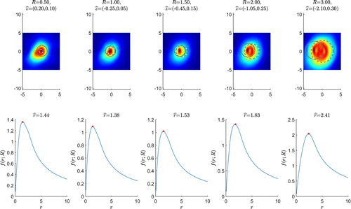
As an illustration of our algorithm, Figure 1 presents the profiles of a kite (dotted line) computed by the EDFM and the corresponding ratio function $f(r;R)$ with different testing radiuses $R\in \{0.1,1,1.5,2,3\}$ for a typical limited aperture data (${\mathrm{\Gamma }}_s={\mathrm{\Gamma }}_m=[0,\pi ]$). The decreasing of $f(r;R)$ as $r\to h^{+}$ and $r\to \mathrm{\infty }$ matches well with the preceding analysis. For a given testing ball (dash line) with either a too small or too large radius R, the reconstructed profile seems to have a much wider disk-shaped region (in red colour) with relatively large W values (in red colour) surrounding the true scatterer (dotted line). We mention that the definition of the ratio function $f(r;R)$ is motivated by the observation that the scatterer profile has a tight support that contains those large values of $W(z;R)$. Based on the graphs of $f(r;R)$ for a given R, we find that its global maximizer (seems to be unique): (15) $\hat{r}\left(R\right)={\text{argmax}}_{r\ge h}f(r;R)$(15) provides an effective estimate of the radius of a covering ball (solid line) that covers the major part of the large values in the profile $W(z;R)$.The numerical value of $\hat{r}$ can be efficiently computed via MATLAB's optimization function fminbnd. Notice that the values of both $\hat{r}$ and $\hat{z}$ are nonlinearly depend on the testing ball radius R (dashed line) and here they are actually estimated in two steps (first find $\hat{z}$ then determine $\hat{r}$). We remark that in our obtained profiles (as images), the transition from the central region (red colour) to the surrounding area (blue colour) is not sharp along the radial direction, hence it is not suitable to detect a circular ball by the Circle Hough Transform [49] algorithm, which is widely used in image processing.

Figure 1. The profiles and ratio functions $f(r;R)$ of a kite with a limited aperture data and different R.

Inspired by the main Theorem 3.1 in [39], we would expect that such a covering ball centred at $\hat{z}\left(R\right)$ with radius $\hat{r}\left(R\right)$, provides some critical feedback to our initial chosen testing ball of radius R, and hence it is natural to update the value of R according to the value of $\hat{r}\left(R\right)$. Based on our extensive numerical experiments, we propose a simple heuristic but effective strategy to adjust R until the difference $|R-\hat{r}\left(R\right)|$ becomes sufficiently small (for example, less than a given tolerance depending on the noise level δ), which turns out to be very satisfactory when the limited aperture is not too narrow. For very narrow limited aperture data, it is still unclear whether it is possible to accurately estimate such a radius in general.

To be more precise, we look for a fixed point $\hat{R}$ that (approximately) satisfies $\hat{R}=\hat{r}\left(\hat{R}\right).$ Without an explicit expression of the mapping $\hat{r}(\cdot )$, a simple iterative scheme would then be (starting with any initial guess $R_0$, e.g. $R_0=0.1$) $R_{k+1}=\hat{r}\left(R_k\right).$ Numerically, we do observe this simple fixed-point iteration often converges in only a few iterations, but there are also very few cases that no convergence was reached (showing periodic oscillations). In such cases, we can improve the convergence by taking a simple average, that is $R_{k+1}=\frac{R_k+\hat{r}\left(R_k\right)}{2}.$ Nevertheless, the convergence of such an iterative scheme is not guaranteed at this point, since the implicit mapping from $R_k$ to $R_{k+1}$ is highly nonlinear, and may not be a contraction. However, under the assumption that $W(z;R)$ has a compact support and takes large values only within a simply connected domain (as shown in Figure 1), we conjecture this nonlinear mapping is a contraction in the noise-free setting.

We finally summarize the above described EDFM in the above Algorithm 1, where the major for loop (with k from 1 to $k_{max}$) implements the proposed simple iteration for updating the fitting ball radius $R_k$. To be practical, the choice of the stopping tolerance tol should be based on the noise level. The rational behind such an iterative scheme, as illustrated in Figure 1, is to approximately match the testing ball's radius R with the fitting ball's radius $\hat{R}$, through the heuristically computed covering ball's radius $\hat{r}$ given by (15(15) $\hat{r}\left(R\right)={\text{argmax}}_{r\ge h}f(r;R)$(15) ). Notice that we have purposely defined three distinct terms for the different balls used in the algorithm: (i) the testing ball, which refers to the ball centred at origin with radius R that is used for generating the exact far-field data; (ii) the covering ball, which refers to the ball centred at $\hat{z}$ with radius $\hat{r}\left(R\right)$ that is computed at each iteration for covering the majority of the large values of indicator function; (iii) the fitting ball, which refers to the final ball centred at $\hat{z}$ with radius $\hat{R}$ that is constructed via the iterative scheme for fitting the scatterer. In our algorithm, we iteratively update the testing ball radius based on the radius of the covering ball to generate a number sequence $\{R_k{\}}_{k=0}^{\mathrm{\infty }}$. If the mapping $\hat{r}(\cdot )$ is assumed to be a contraction, this sequence is expected to be convergent and hence the iterative algorithm will eventually lead to a final fitting ball, which provides an estimated location and size (but not shape) of the scatterer.

4. Numerical results

In this section, we provide several 2D inverse acoustic scattering examples from impenetrable and sound-soft obstacles to demonstrate the effectiveness of our proposed method. All simulations are implemented using MATLAB 2017b on a Dell Precision workstation with Intel(R) Core(TM) i7-7700K [email protected] and 32GB RAM. To simulate the measurement noise, we added random noise to the far-field data F according to $F^{\delta }=F+\delta \parallel F\parallel \frac{S_1+S_{2}i}{\parallel S_1+S_{2}i\parallel },$ where $S_1$ and $S_2$ are two $N\times N$ random matrices (with a standard normal distribution) generated by the MATLAB function randn(N,N). Here the value of δ represents the level of noise based on relative error. In our numerical simulations, we choose the wave number $\kappa =3$ (with wavelength $\lambda =2\pi /\kappa \approx 2.1$), the total number of full aperture incident and observation directions N=64, the noise level $\delta =10\mathrm{\%}$, the sampling domain is $[-a,a{]}^2$ with a=5, the sampling mesh size n=200, the initial radius guess $R_0=0.1$, the stopping tolerance tol=0.1, and the maximum number of iterations $k_{max}=100$. We have also numerically implemented and tested the multilevel ESM in [39], but its estimated radius was very sensitive in terms of the selection of the initial guess and the level of noise in the data. Therefore, in order to keep the discussion fair, we elected not to include it in this paper. We would like to point out here once again that our proposed method, EDFM, doesn't suffer from such type of issues and hence is more attractive to practical applications.

We used the Nyström method [2] to generate synthetic far-field data for the following four impenetrable scatterers (with Dirichlet boundary condition) centred at the origin:

1. A circle with centre $(0,0)$ and radius 2 given by: $\left(x\right(t),y(t\left)\right)=2(\cos t,\sin t),0\le t\le 2\pi .$

2. A triangle given by the parametric equations: $\left(x\right(t),y(t\left)\right)=(1+0.15\cos 3t)(\cos t,\sin t),0\le t\le 2\pi .$

3. A single kite given by the parametric equations: $\left(x\right(t),y(t\left)\right)=(\cos t+0.65(\cos 2t-1),1.5\sin t),0\le t\le 2\pi .$

4. A peanut given by the parametric equations:: $\left(x\right(t),y(t\left)\right)=\sqrt{4{\cos }^{2}t+{\sin }^{2}t}(\cos t,\sin t),0\le t\le 2\pi .$

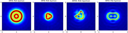
For comparison, Figure 2 shows the true scatterers (dotted line) and their reconstructed profiles by the DFM with a full aperture data. As expected, the scatterers are very accurately identified by their DFM profiles.

Figure 2. The reconstructed profile of the true scatterers by the DFM with full aperture data.

4.1. Backward scattering geometries

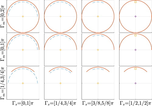
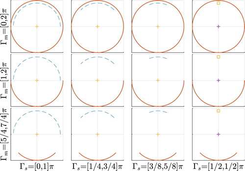
The first group of limited aperture data are specified by combining the given incident directions ${\mathrm{\Gamma }}_s\in \left\{\right[0,\pi ],[\pi /4,3\pi /4],[3\pi /8,5\pi /8],\{\pi /2\left\}\right\}$ with the following backward scattering observation directions ${\mathrm{\Gamma }}_m\in \left\{\right[0,2\pi ],[0,\pi ],[\pi /4,3\pi /4\left]\right\}$, as shown in Figure 3. Notice that the single incident direction case is marked as an empty square. We will report the reconstruction of each scatterer for all combinations and then compare their accuracy in a single figure, corresponding to geometries depicted in Figure 3.

Figure 3. Backward scattering: combinations of incident (dashed line) and observation (solid line) directions.

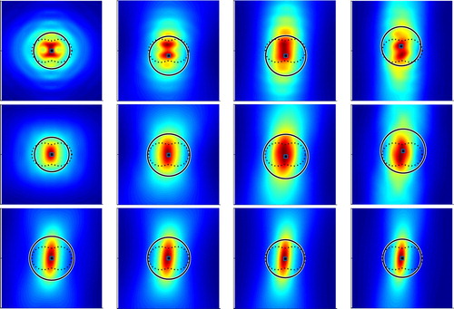
In Figures 4–7, the reconstructed balls and profiles with different combinations of backward scattering limited aperture data are plotted for each scatterer, respectively. Notice here that we have included the case (the first row) with full aperture data (i.e. ${\mathrm{\Gamma }}_m=[0,2\pi ]$) for the sake of comparison. In most cases, the reconstructed balls (solid line) seem to very accurately match the location and size of the true scatters (dotted line), and only occasionally the ball centre (solid square in black) slightly deviates from the scatterer centre. This mainly happens for the case of narrow limited aperture data (the last row) and one incident direction (the last column). In addition, the underlying indicator function profile suggests that the centre of the reconstructed ball accurately lies within the large values of $W(z;R)$. This implies that our iterative scheme works very well in estimating the ball radius, in spite of the possible inaccurate location of the ball centre due to very limited aperture data. The perfect fitting of the reconstructed ball with the scatterer (circle) in Figure 4 shows the great potential of our proposed method. This scatterer also serves as the benchmark for calibrating our iterative algorithm for better estimating the radius. Figure 5 with the triangle demonstrates the fitting ball may slightly overestimate the actual size of the scatterer, although the reconstruction quality is satisfactory in most cases. Figure 6 with the kite tells the reconstructed fitting ball could catch the irregular shaped scatterer in all cases. Figure 7 with the peanut indicates the reconstructed fitting ball tends to cover the whole scatterer along the major axis direction.

Figure 4. The reconstructions of the circle with backward-scattering limited aperture data.

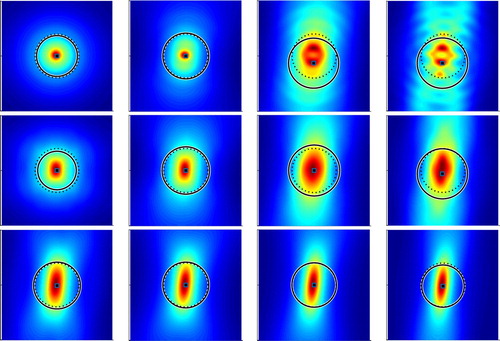
Figure 5. The reconstructions of the triangle with backward-scattering limited aperture data.

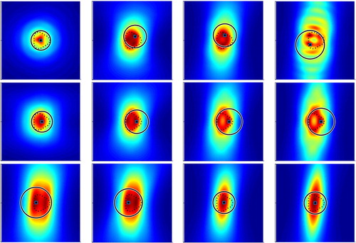
Figure 6. The reconstructions of the kite with backward-scattering limited aperture data.

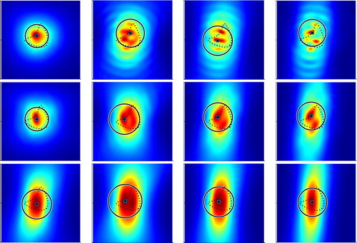
Figure 7. The reconstructions of the peanut with backward-scattering limited aperture data.

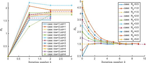
To demonstrate the convergence behaviour of the iterative scheme for estimating the ball radius, Figure 8 shows the convergence history of the values of the estimated radius $R_k$ for the kite under different combinations of limited aperture data and different initial guesses $R_0$, respectively. In the left subplot of Figure 8, each curve corresponds to a different type of limited aperture data with the same initial guess $R_0=0.1$. For simplicity, we denote each case depicted in Figure 3 according to its row and column number as ‘case: row=i,col=j’ with i=1,2,3 and j=1,2,3,4. It appears that for each case the corresponding iterations numerically converge to a marginally different value that always lies within 1.5 and 2.2 and hence indeed correctly capture the best radius that fits the scatterer which in this case is about 1.6–1.8. From the other hand, on the right subplot of Figure 8, each curve corresponds to a tighter tolerance (tol=0.01) and the same limited aperture angles (${\mathrm{\Gamma }}_s={\mathrm{\Gamma }}_m=[0,\pi ]$), but with different initial guess of radius $R_0\in \{0.5,1,1.5,2,2.5,3,3.5,4,4.5,5\}$. Clearly, our proposed iterative scheme exhibits rapid convergence to the same radius and is very robust with respect to various initial guesses, even in the presence of $\delta =10\mathrm{\%}$ level of noise. Such a robust convergence property is particularly useful, since the exact size of the scatterer is unknown in practice and the far-field data also contains unknown noise.

Figure 8. The convergence history of the iterative scheme for estimating the fitting ball radius of the kite with different limited aperture data (left, 12 cases) and different initial radius guess (right, 10 cases).

To illustrate the effects of the wave numbers and noise levels on our proposed EDFM, Figure 9 shows the reconstructed fitting ball for the kite with different wave numbers $\kappa =1,3,5,7,9$ for a fixed backward-scattering limited aperture data (${\mathrm{\Gamma }}_s=[3\pi /8,5\pi /8]$ and ${\mathrm{\Gamma }}_m=[\pi /4,3\pi /4]$, i.e. case: row=3,col=3 in Figure 3), and Figure 10 displays the reconstructed fitting ball for the kite with $\kappa =3$ and different levels of noise $\delta =10\mathrm{\%},20\mathrm{\%},30\mathrm{\%},40\mathrm{\%},50\mathrm{\%}$. Both figures demonstrate the proposed EDFM performs well for a range of wave numbers and noise levels, although the reconstruction accuracy is slightly different in each setting.

Figure 9. The reconstructions of the kite with different wave numbers $\kappa =1,3,5,7,9$ for a fixed backward-scattering limited aperture data (${\mathrm{\Gamma }}_s=[3\pi /8,5\pi /8]$ and ${\mathrm{\Gamma }}_m=[\pi /4,3\pi /4]$).

Figure 10. The reconstructions of the kite with $\kappa =3$ and different levels of noise $\delta =10\mathrm{\%},20\mathrm{\%},30\mathrm{\%},40\mathrm{\%},50\mathrm{\%}$ for a fixed backward-scattering limited aperture data (${\mathrm{\Gamma }}_s=[3\pi /8,5\pi /8]$ and ${\mathrm{\Gamma }}_m=[\pi /4,3\pi /4]$).

4.2. Forward scattering geometries

The second group of the limited aperture data is specified by combining the given incident directions ${\mathrm{\Gamma }}_s\in \left\{\right[0,\pi ],[\pi /4,3\pi /4],[3\pi /8,5\pi /8],\{\pi /2\left\}\right\}$ with the following forward scattering observation directions ${\mathrm{\Gamma }}_m\in \left\{\right[0,2\pi ],[\pi ,2\pi ],[5\pi /4,7\pi /4\left]\right\}$, as shown in Figure 11. The limited aperture observation directions are now located at the opposite side of the incident directions, which is expected to be more difficult due to the impenetrable obstacles.

Figure 11. Forward scattering: combinations of incident (dashed line) and observation (solid line) directions.

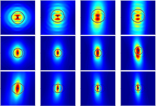
In Figures 12–15, the reconstructed balls and profiles with different combinations of forward scattering limited aperture data are plotted for each scatterer, respectively. The overall reconstruction quality is slightly worse compared to the previous backward scattering cases. Here we do observe issues with overestimating or underestimating the ball radius for the case of narrow limited aperture data (the last row). This may be explained by the fact that for the cases in discussion the scatterer largely blocks incident waves and hence the measured limited aperture far-field data contain very limited and incomplete information regarding the scatterer's shape. In this perspective, it is even desirable to get an overestimated ball that could account for the uncertainty in the far-field data regarding the true location and size of the scatterer. It is a common practice to further improve the reconstruction accuracy by using multifrequency data for a range of different wave numbers.

Figure 12. The reconstructions of the circle with forward-scattering limited aperture data.

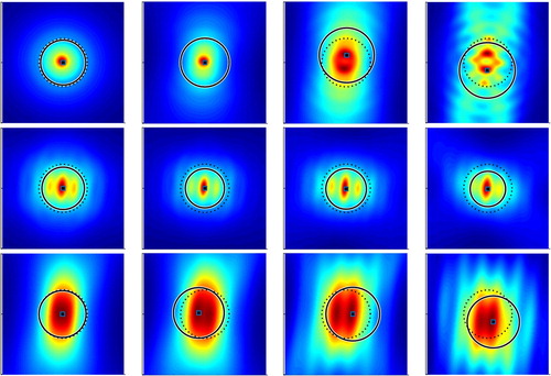
Figure 13. The reconstructions of the triangle with forward-scattering limited aperture data.

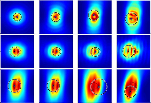
Figure 14. The reconstructions of the kite with forward-scattering limited aperture data.

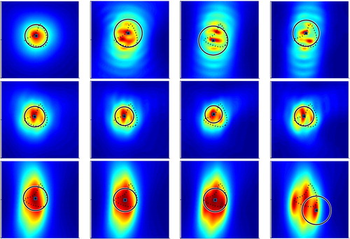
Figure 15. The reconstructions of the peanut with forward-scattering limited aperture data.

5. Conclusion

In this paper, we proposed a novel extended direct factorization method (EDFM) for qualitatively solving inverse scattering problems with limited aperture data. The proposed EDFM generalizes the extended sampling method to the framework of the direct factorization method, where a new iterative scheme is developed for estimating the ball radius. Numerical results with limited aperture data are presented to illustrate the promising performance of the proposed EDFM. An inexpensive estimation of a fitting ball presented in this paper closely fits the unknown scatterer, which can also serve as a good initial guess for locally convergent nonlinear optimization algorithms and Bayesian method [50].

Our future work include the development of more robust techniques for estimating the centre of the fitting ball and assembling the multiple incident directions data. In the setting of very limited aperture data, the currently used global maximum/minimum of the reconstructed profile seems likely to significantly deviate from the true scatterer centre. The straightforward summation of the indicator function for multiple incident directions data may not be the most effective way to obtain an improved reconstruction profile than a single incident direction. For the case with multiple connected scatterers, the current approach seems to not directly applicable to reconstruct their locations and sizes, which deserves further studies.

Following the idea of ESM, it is possible to fit a scatterer by any desirable shape (e.g. an ellipse or a triangle), which may be able to better reconstruct non-round shape scatterers (e.g. peanut). Nevertheless, we remark that the simple circle (or ball) is preferred since: (i) it has an exact formula for generating far-field pattern A; (ii) it is invariant under rotation about the centre; and (iii) only one degree of freedom (i.e. the radius) is required to compute once the centre is determined. It would be interesting to gradually ‘learn’ a good testing geometry (other than a ball) from the limited aperture data within the framework of ESM.

Acknowledgments

The authors appreciate the two anonymous referees for their valuable comments and detailed suggestions that have greatly contributed to improving the quality of this paper. The authors also would like to thank Dr. Juan Liu and Dr. Jiguang Sun for some inspiring discussion and generously sharing with us their multilevel ESM codes.

Disclosure statement

No potential conflict of interest was reported by the authors.

ORCID

Jun Liu http://orcid.org/0000-0003-1904-2350

References

- Colton D, Coyle J, Monk P. Recent developments in inverse acoustic scattering theory. SIAM Rev. 2000;42:369–414. doi: 10.1137/S0036144500367337
- Colton D, Kress R. Inverse acoustic and electromagnetic scattering theory. New York: Springer; 2012.
- Ammari H, Chow YT, Zou J. Phased and phaseless domain reconstructions in the inverse scattering problem via scattering coefficients. SIAM J Appl Math. 2016;76:1000–1030. doi: 10.1137/15M1043959
- Cakoni F, Rezac JD. Direct imaging of small scatterers using reduced time dependent data. J Comput Phys. 2017;338:371–387. doi: 10.1016/j.jcp.2017.02.061
- Fotopoulos G, Harju M. Inverse scattering with fixed observation angle data in 2D. Inverse Problems Sci Eng. 2016;25:1492–1507. doi: 10.1080/17415977.2016.1267170
- Guo Y, Hmberg D, Hu G, et al. A time domain sampling method for inverse acoustic scattering problems. J Comput Phys. 2016;314:647–660. doi: 10.1016/j.jcp.2016.03.046
- Li J, Liu H, Wang Q. Enhanced multilevel linear sampling methods for inverse scattering problems. J Comput Phys. 2014;257:554–571. doi: 10.1016/j.jcp.2013.09.048
- Liu K, Xu Y, Zou J. A parallel radial bisection algorithm for inverse scattering problems. Inverse Prob Sci Eng. 2013;21:197–209. doi: 10.1080/17415977.2012.686498
- Liu X. A novel sampling method for multiple multiscale targets from scattering amplitudes at a fixed frequency. Inverse Prob. 2017;33:085011.
- Liu X, Zhang B. Recent progress on the factorization method for inverse acoustic scattering problems. SCIENTIA SINICA Math. 2015;45:873–890.
- Giorgi G, Brignone M, Aramini R, et al. Application of the inhomogeneous Lippmann–Schwinger equation to inverse scattering problems. SIAM J Appl Math. 2013;73:212–231. doi: 10.1137/120869584
- Murch RD, Tan DGH, Wall DJN. Newton-Kantorovich method applied to two-dimensional inverse scattering for an exterior Helmholtz problem. Inverse Prob. 1988;4:1117–1128. doi: 10.1088/0266-5611/4/4/012
- Roger A. Newton-kantorovitch algorithm applied to an electromagnetic inverse problem. IEEE Trans Antennas Propagat. 1981;29:232–238. doi: 10.1109/TAP.1981.1142588
- Arens T, Lechleiter A. The linear sampling method revisited. J Integral Equ Appl. 2009;21:179–202. doi: 10.1216/JIE-2009-21-2-179
- Cakoni F, Colton D. A qualitative approach to inverse scattering theory. New York: Springer; 2013.
- Colton D, Haddar H, Piana M. The linear sampling method in inverse electromagnetic scattering theory. Inverse Prob. 2003;19:S105–S137. doi: 10.1088/0266-5611/19/6/057
- Potthast R. A survey on sampling and probe methods for inverse problems. Inverse Prob. 2006;22:R1–R47. doi: 10.1088/0266-5611/22/2/R01
- Cakoni F, Colton D, Monk P. The linear sampling method in inverse electromagnetic scattering. Philadelphia (PA): SIAM; 2011.
- Kirsch A, Grinberg N. The factorization method for inverse problems. Oxford: OUP; 2008.
- Ito K, Jin B, Zou J. A direct sampling method to an inverse medium scattering problem. Inverse Prob. 2012;28:025003. doi: 10.1088/0266-5611/28/2/025003
- Bellis C, Bonnet M, Cakoni F. Acoustic inverse scattering using topological derivative of far-field measurements-basedL2cost functionals. Inverse Prob. 2013;29:075012. doi: 10.1088/0266-5611/29/7/075012
- Bonnet M, Cakoni F. Analysis of topological derivative as a tool for qualitative identification. Inverse Problems. 2019.
- Lour FL, Rapún M-L. Topological sensitivity for solving inverse multiple scattering problems in three-dimensional electromagnetism. part i: One step method. SIAM J Imag Sci. 2017;10:1291–1321. doi: 10.1137/17M1113850
- Lour FL, Rapún M-L. Topological sensitivity for solving inverse multiple scattering problems in three-dimensional electromagnetism. part II: Iterative method. SIAM J Imag Sci. 2018;11:734–769. doi: 10.1137/17M1148359
- Yuan H, Bracq G, Lin Q. Inverse acoustic scattering by solid obstacles: topological sensitivity and its preliminary application. Inverse Problems Sci Eng. 2015;24:92–126. doi: 10.1080/17415977.2015.1017483
- Leem KH, Liu J, Pelekanos G. Two direct factorization methods for inverse scattering problems. Inverse Prob. 2018;34:125004.
- Leem KH, Liu J, Pelekanos G. An adaptive quadrature-based factorization method for inverse acoustic scattering problems. Inverse Problems Sci Engin. 2019;27(3):299–316. doi: 10.1080/17415977.2018.1459600
- Bao G, Liu J. Numerical solution of inverse scattering problems with multi-experimental limited aperture data. SIAM J Sci Comput. 2003;25:1102–1117. doi: 10.1137/S1064827502409705
- Barucq H, Bekkey C, Djellouli R. A multi-step procedure for enriching limited two-dimensional acoustic far-field pattern measurements. J Inverse Ill-posed Prob. 2010;18.
- Barucq H, Bekkey C, Djellouli R. Full aperture reconstruction of the acoustic far-field pattern from few measurements. Commun Comput Phys. 2012;11:647–659. doi: 10.4208/cicp.281209.150610s
- Djellouli R, Tezaur R, Farhat C. On the solution of inverse obstacle acoustic scattering problems with a limited aperture. Mathematical and Numerical Aspects of Wave Propagation WAVES 2003, Springer Berlin Heidelberg, 2003, pp. 625–630.
- Ochs Jr RL. The limited aperture problem of inverse acoustic scattering: Dirichlet boundary conditions. SIAM J Appl Math. 1987;47:1320–1341. doi: 10.1137/0147087
- You Y-X, Miao G-P, Liu Y-Z. A numerical method for solving the limited aperture problem in three-dimensional inverse obstacle scattering. Int J Nonlinear Sci Numer Simul. 2001;2. doi: 10.1515/IJNSNS.2001.2.1.29
- Zinn A. On an optimisation method for the full- and the limited-aperture problem in inverse acoustic scattering for a sound-soft obstacle. Inverse Prob. 1989;5:239–253. doi: 10.1088/0266-5611/5/2/009
- Ikehata M, Niemi E, Siltanen S. Inverse obstacle scattering with limited-aperture data. Inverse Prob Imag. 2012;6:77–94. doi: 10.3934/ipi.2012.6.77
- Audibert L, Haddar H. A generalized formulation of the linear sampling method with exact characterization of targets in terms of farfield measurements. Inverse Prob. 2014;30:035011. doi: 10.1088/0266-5611/30/3/035011
- Audibert L, Haddar H. The generalized linear sampling method for limited aperture measurements. SIAM J Imag Sci. 2017;10:845–870. doi: 10.1137/16M110112X
- Liu X, Sun J. Data recovery in inverse scattering: from limited-aperture to full-aperture. J Comput Phys. 2019;386:350–364. doi: 10.1016/j.jcp.2018.10.036
- Liu J, Sun J. Extended sampling method in inverse scattering. Inverse Prob. 2018;34:085007. doi: 10.1088/1361-6420/aaca90
- Potthast R, Sylvester J, Kusiak S. A range test for determining scatterers with unknown physical properties. Inverse Prob. 2003;19:533–547. doi: 10.1088/0266-5611/19/3/304
- Aramini R, Brignone M, Piana M. The linear sampling method without sampling. Inverse Prob. 2006;22:2237–2254. doi: 10.1088/0266-5611/22/6/020
- Benning M, Burger M. Modern regularization methods for inverse problems. Acta Numer. 2018;27:1–111. doi: 10.1017/S0962492918000016
- Brignone M, Bozza G, Aramini R, et al. A fully no-sampling formulation of the linear sampling method for three-dimensional inverse electromagnetic scattering problems. Inverse Prob. 2008;25:015014.
- Harris I, Kleefeld A. Analysis of new direct sampling indicators for far-field measurements. Inverse Prob. 2019;35:054002. doi: 10.1088/1361-6420/ab08be
- Liu H, Zou J. Zeros of the bessel and spherical bessel functions and their applications for uniqueness in inverse acoustic obstacle scattering. IMA J Appl Math. 2007;72:817–831. doi: 10.1093/imamat/hxm013
- Ben-Israel A, Charnes A. Contributions to the theory of generalized inverses. J Soc Ind Appl Math. 1963;11:667–699. doi: 10.1137/0111051
- Climent J-J, Thome N, Wei Y. A geometrical approach on generalized inverses by neumann-type series. Linear Algebra Appl. 2001;332–334:533–540. doi: 10.1016/S0024-3795(01)00309-3
- Tanabe K. Neumann-type expansion of reflexive generalized inverses of a matrix and the hyperpower iterative method. Linear Algebra Appl. 1975;10:163–175. doi: 10.1016/0024-3795(75)90008-7
- Atherton T, Kerbyson D. Size invariant circle detection. Image Vision Comput. 1999;17:795–803. doi: 10.1016/S0262-8856(98)00160-7
- Li Z, Deng Z, Sun J. Limited aperture inverse scattering problems using Bayesian approach and extended sampling method. arXiv e-prints, (2019), p. arXiv:1905.12222.