Numerical differentiation for two-dimensional functions by a Fourier extension method

ABSTRACT

Based on the idea of Fourier extension, we develop a new method for numerical differentiation of two-dimensional functions on an arbitrary domain. The function will be extended to a periodic function on a larger domain. The Tikhonov regularization method in Hilbert scales is presented to deal with the ill-posedness of the problem. The Sobolev norm defined on the larger domain will be used as a stabilizer. An error analysis is provided with a regularization parameter chosen by a discrepancy principle. Numerical experiments are also presented to illustrate the effectiveness of the proposed method.

KEYWORDS:

• Ill-posed problem
• regularization
• numerical differentiation
• Fourier extension

2010 MATHEMATICS SUBJECT CLASSIFICATION:

• 47A52

1. Introduction

Numerical differentiation is an interesting topic in the field of numerical analysis. This arises in a lot of mathematical models and engineering problems [1–6]. The main difficulty of numerical differentiation is that it is ill-posed, i.e. the small errors in the input data may lead to huge errors in its approximated derivatives. In the past years, a wide range of computational methods have been reported to treat the numerical differentiation problem [7–20]. According to the types of regularization techniques, these methods can be classified into difference methods, mollification methods, truncation methods and Tikhonov methods. Most of these papers focused on a one-dimensional case, but only a few results on the high dimensional cases have been reported [12,21–24]. In particular, based on radial basis functions approximation [15], the authors used a semi-norm in the global space as the regularization functional on a finite interval. By solving numerically a smoothing functional, a regularization solution based on Green's function was constructed [12]. Wei et al.[21] gave a regularization algorithm for reconstruction of numerical derivatives from two-dimensional scattered noisy data based on the thin plate spline approximation theory.

In [23], a truncated Fourier series method was proposed for the numerical differentiation of 2D periodic functions. This method is effective for calculating arbitrary derivatives of periodic functions. However, the situation changes completely when the function is non-periodic. The reason lies in the well-known Gibbs phenomenon, and rapid convergence of Fourier series is available only for periodic functions. Recently, Fourier extension method has attracted more and more attentions of the researchers [25–30]. It has been proved successfully to ameliorate the Gibbs phenomenon. If a function $f\in H^p({\mathrm{\Omega }}_2)$, the idea of the Fourier extension is to extend the function f to the function g that is periodic on a rectangular domain ${\mathrm{\Omega }}_1\supset {\mathrm{\Omega }}_2$.

For numerical differentiation, our aim is to obtain approximation derivatives of f from its perturbed data $f^{\delta }$ satisfying (1) $\Vert f-f^{\delta }{\Vert }_{L^2({\mathrm{\Omega }}_1)}\le \delta ,$(1) where $\delta >0$ is a given constant called the error level. In this paper, we construct an approximation function f by using the Fourier extension method. Considering the features of numerical differentiation problems, we present a modified Tikhonov regularization method to obtain a stable Fourier extension. The Sobolev norm defined on a larger domain will be used as a stabilizer, and an error analysis is provided when we choose the regularization parameter by a discrepancy principle.

The structure of the paper is as follows. In Section 2, we present the mathematical formulation of the Fourier extension by using the Tikhonov method. The choice of the regularization parameter and corresponding convergence results are shown in Section 3. Section 4 provides a variety of numerical results to demonstrate the effectiveness of our method.

2. Formulation of problem and solution

We first introduce some notations. Let ${\mathrm{\Omega }}_1=(-\pi ,\pi )\times (-\pi ,\pi )$ and ${\mathrm{\Omega }}_2$ be a subdomain of ${\mathrm{\Omega }}_1$. Let $\mathbf{x}=(x_1,x_2)$, $\mathbf{l}=(l_1,l_2)$ and $l_i$ be integers. Set $|\mathbf{l}|=max\{|l_1|,|l_2|\}$ and $\mathbf{l}\cdot \mathbf{x}=l_1{x}_1+l_2{x}_2$. Next, let $\mathbb{N}$ be the set of all non-negative integers. For any two-tuples $\alpha =({\alpha }_1,{\alpha }_2)\in {\mathbb{N}}^2$, $|\alpha {|}_1={\alpha }_1+{\alpha }_2$. The notation ${\mathrm{\partial }}_j$ stands for $\mathrm{\partial }/\mathrm{\partial }{x}_j$ and $D^{\alpha }f={\mathrm{\partial }}_{x_1}^{{\alpha }_1}{\mathrm{\partial }}_{x_2}^{{\alpha }_2}f$. For any positive integer q, we define $D^{q}f=\{D^{\alpha }f:|\alpha {|}_1=q\}$ and (2) $|D^{q}f|={\left(\sum _{|\alpha {|}_1=q}|D^{\alpha }f{|}^2\right)}^{1/2}.$(2) $\Vert \cdot {\Vert }_{s,{\mathrm{\Omega }}_k},k=1,2,$ denotes the norm in Sobolev space $H^s({\mathrm{\Omega }}_k),$ and we defined $\Vert \cdot {\Vert }_{s,{\mathrm{\Omega }}_k},k=1,2$ as (3) $\Vert f{\Vert }_{s,{\mathrm{\Omega }}_i}:={({\int }_{{\mathrm{\Omega }}_i}(|f{|}^2+|D^{s}f{|}^2))}^{1/2},$(3) where s = 0 and $\Vert \cdot {\Vert }_{0,{\mathrm{\Omega }}_k}$ denotes the $L^2({\mathrm{\Omega }}_k)$ norm. Let $H_p^s({\mathrm{\Omega }}_1)$ be the subspace of $H^s({\mathrm{\Omega }}_1)$ containing all functions with period $2\pi$ for all variables.

Fourier transformation of a function $f\in L^2({\mathrm{\Omega }}_1)$ is (4) $\mathcal{F}[f(\mathbf{x})]=\sum _{|\mathbf{l}|=0}^{\mathrm{\infty }}{\mathbf{f}}_{\mathbf{l}}{e}^{i\mathbf{l}\cdot \mathbf{x}}$(4) with the Fourier coefficients (5) ${\mathbf{f}}_{\mathbf{l}}=\frac{1}{4{\pi }^2}{\int }_{{\mathrm{\Omega }}_1}f(\mathbf{x})e^{-i\mathbf{l}\cdot \mathbf{x}}\mathrm{d}\mathbf{x}.$(5) Accordingly, for any vector $\mathbf{v}=\{v_{\mathbf{l}}{\}}_{|\mathbf{l}|=0}^{\mathrm{\infty }}\in l^2$, we define the operator (6) $(\mathcal{F}\mathbf{v})(\mathbf{x})=\sum _{|\mathbf{l}|=0}^{\mathrm{\infty }}{v}_{\mathbf{l}}{e}^{i\mathbf{l}\cdot \mathbf{x}}$(6) and (7) $({\mathcal{P}}_N\mathbf{v})(\mathbf{x})=\sum _{|\mathbf{l}|=0}^N{v}_{\mathbf{l}}{e}^{i\mathbf{l}\cdot \mathbf{x}}$(7) Suppose that we know the perturbed data $f^{\delta }$ of $f\in L^2({\mathrm{\Omega }}_2)$ satisfying (8) $\Vert f^{\delta }-f{\Vert }_{0,{\mathrm{\Omega }}_2}\le \delta ,$(8) where $\delta >0$ is a given error level; our aim is to obtain approximation derivatives of f from $f^{\delta }$.

By using the Tikhonov regularization method, we treat this problem as follows: define a cost functional (9) $\mathrm{\Phi }(\mathbf{v})=\Vert \mathcal{F}\mathbf{v}-f^{\delta }{\Vert }_{0,{\mathrm{\Omega }}_2}^2+\beta \Vert \mathcal{F}\mathbf{v}{\Vert }_{q,{\mathrm{\Omega }}_1}^2,$(9) where β is a regularization parameter and q is a positive integer. If we let (10) $d_q(\mathbf{l})={[1+\sum _{|\alpha {|}_1=q}\sum _{|\mathbf{l}|=0}^{\mathrm{\infty }}|l_1{|}^{2{\alpha }_1}|l_2{|}^{2{\alpha }_2}]}^{1/2}\text{and}{\mathcal{D}}_q\mathbf{v}=[d_q(\mathbf{l})v_{\mathbf{l}}],$(10) then we can verify that (11) $\Vert \mathcal{F}\mathbf{v}{\Vert }_{q,{\mathrm{\Omega }}_1}=\frac{1}{2\pi }\Vert {\mathcal{D}}_q\mathbf{v}{\Vert }_{l^2}.$(11) So cost functional (9(9) $\mathrm{\Phi }(\mathbf{v})=\Vert \mathcal{F}\mathbf{v}-f^{\delta }{\Vert }_{0,{\mathrm{\Omega }}_2}^2+\beta \Vert \mathcal{F}\mathbf{v}{\Vert }_{q,{\mathrm{\Omega }}_1}^2,$(9) ) can be converted to (12) $\mathrm{\Phi }(\mathbf{v})=\Vert \mathcal{F}\mathbf{v}-f^{\delta }{\Vert }_{0,{\mathrm{\Omega }}_2}^2+\beta \Vert {\mathcal{D}}_q\mathbf{v}{\Vert }_{l^2}^2.$(12) Now if ${\mathbf{v}}_{\beta }^{\delta }$ is the minimizer of the functional Φ, then (13) $f_{\beta }^{\delta }=\mathcal{F}{\mathbf{v}}_{\beta }^{\delta }$(13) will be chosen as the approximate function of f. It is well known that ${\mathbf{v}}_{\beta }^{\delta }$ can be obtained by solving the following equation [31] (14) $({\mathcal{F}}^{\ast }\mathcal{F}+\beta {\mathcal{D}}_q^2)\mathbf{v}={\mathcal{F}}^{\ast }{f}^{\delta }.$(14)

Remark

${\mathcal{D}}_q$ is a diagonal matrix. The method can be easily implemented because of the Fourier transformation's differential properties.

Moreover, if we let $g_{\beta }(\lambda )=1/(\lambda +\beta )$ and $\mathcal{T}=\mathcal{F}{\mathcal{D}}_q^{-1}$, then (15) ${\mathbf{v}}_{\beta }^{\delta }={\mathcal{D}}_q^{-1}{g}_{\beta }({\mathcal{T}}^{\ast }\mathcal{T}){\mathcal{T}}^{\ast }{f}^{\delta },$(15) and the following lemma holds.

Remark 2.1

It is well known that the function $g_{\beta }(\lambda )$ has the following properties.

Lemma 2.2

[32]

(16) $\underset{\lambda >0}{sup}{\lambda }^{1/2}|g_{\beta }(\lambda )|\le \frac{1}{2\sqrt{\beta }},\underset{\lambda >0}{sup}\lambda |g_{\beta }(\lambda )|\le 1$(16) and (17) $\underset{\lambda >0}{sup}{\lambda }^{1/2}|1-\lambda g_{\beta }(\lambda )|\le \frac{\sqrt{\beta }}{2},\underset{\lambda >0}{sup}|1-\lambda g_{\beta }(\lambda )|\le 1.$(17)

By using the extension theorem in Sobolev spaces [33] and cut-off functions in [34,35], we can give the following lemma.

Lemma 2.3

For any $f\in H^s({\mathrm{\Omega }}_2),$ there exists a function $\hat{f}\in H_p^s({\mathrm{\Omega }}_1)$ such that (18) $\hat{f}(x)=f(x)\mathrm{\forall }x\in {\mathrm{\Omega }}_2\text{and}\Vert \hat{f}{\Vert }_{s,{\mathrm{\Omega }}_1}\le E$(18) with some constant E.

Lemma 2.4

Suppose that $f\in H^s({\mathrm{\Omega }}_2)$ and $\hat{f}$ is defined above, and the vector $\hat{\mathbf{v}}=\{{\hat{\mathbf{f}}}_{\mathbf{l}}{\}}_{|\mathbf{l}|=0}^{\mathrm{\infty }}$ contains all the Fourier coefficients of $\hat{f};$ if we let ${\hat{\mathbf{v}}}_N={\mathcal{P}}_N\hat{\mathbf{v}},$ then for $q\ge s$ (19) $\Vert \hat{\mathbf{v}}-{\hat{\mathbf{v}}}_N{\Vert }_{l^2}\le N^{-s}E\text{and}\Vert {\mathcal{D}}_q{\hat{\mathbf{v}}}_N{\Vert }_{l^2}\le \frac{q}{s}{N}^{q-s}E,$(19)

Proof.

(20) $\begin{array}{rl}\Vert \hat{\mathbf{v}}-{\hat{\mathbf{v}}}_N{\Vert }_{l^2}& =\Vert (I-{\mathcal{P}}_N)\hat{\mathbf{v}}{\Vert }_{l^2}^2=\sum _{|\mathbf{l}|=N+1}^{\mathrm{\infty }}{\hat{\mathbf{f}}}_{\mathbf{l}}^2\\ & =N^{-2s}\sum _{|\mathbf{l}|=N+1}^{\mathrm{\infty }}{N}^{2s}{\hat{\mathbf{f}}}_{\mathbf{l}}^2\\ & \le N^{-2s}\sum _{|\mathbf{l}|=N+1}^{\mathrm{\infty }}[d_s(\mathbf{l}){]}^2{\hat{\mathbf{f}}}_{\mathbf{l}}^2\\ & \le N^{-2s}\sum _{|\mathbf{l}|=0}^{\mathrm{\infty }}[d_s(\mathbf{l}){]}^2{\hat{\mathbf{f}}}_{\mathbf{l}}^2\\ & =N^{-2s}\Vert {\mathcal{D}}_s\hat{\mathbf{v}}{\Vert }_{l^2}^2\end{array}$(20) and (21) $\begin{array}{rl}\Vert {\mathcal{D}}_q{\hat{\mathbf{v}}}_N{\Vert }_{l^2}^2& =\sum _{|\mathbf{l}|=0}^N[d_q(\mathbf{l}){]}^2{\hat{\mathbf{f}}}_{\mathbf{l}}^2\\ & \le \frac{q}{s}{N}^{2(q-s)}\sum _{|\mathbf{l}|=0}^N[d_s(\mathbf{l}){]}^2{\hat{\mathbf{f}}}_{\mathbf{l}}^2\\ & \le \frac{q}{s}{N}^{2(q-s)}\Vert {\mathcal{D}}_s\mathbf{v}{\Vert }_{l^2}^2\end{array}$(21) The assertion of the lemma follows from (11(11) $\Vert \mathcal{F}\mathbf{v}{\Vert }_{q,{\mathrm{\Omega }}_1}=\frac{1}{2\pi }\Vert {\mathcal{D}}_q\mathbf{v}{\Vert }_{l^2}.$(11) ), (18(18) $\hat{f}(x)=f(x)\mathrm{\forall }x\in {\mathrm{\Omega }}_2\text{and}\Vert \hat{f}{\Vert }_{s,{\mathrm{\Omega }}_1}\le E$(18) ), (20(20) $\begin{array}{rl}\Vert \hat{\mathbf{v}}-{\hat{\mathbf{v}}}_N{\Vert }_{l^2}& =\Vert (I-{\mathcal{P}}_N)\hat{\mathbf{v}}{\Vert }_{l^2}^2=\sum _{|\mathbf{l}|=N+1}^{\mathrm{\infty }}{\hat{\mathbf{f}}}_{\mathbf{l}}^2\\ & =N^{-2s}\sum _{|\mathbf{l}|=N+1}^{\mathrm{\infty }}{N}^{2s}{\hat{\mathbf{f}}}_{\mathbf{l}}^2\\ & \le N^{-2s}\sum _{|\mathbf{l}|=N+1}^{\mathrm{\infty }}[d_s(\mathbf{l}){]}^2{\hat{\mathbf{f}}}_{\mathbf{l}}^2\\ & \le N^{-2s}\sum _{|\mathbf{l}|=0}^{\mathrm{\infty }}[d_s(\mathbf{l}){]}^2{\hat{\mathbf{f}}}_{\mathbf{l}}^2\\ & =N^{-2s}\Vert {\mathcal{D}}_s\hat{\mathbf{v}}{\Vert }_{l^2}^2\end{array}$(20) ) and (21(21) $\begin{array}{rl}\Vert {\mathcal{D}}_q{\hat{\mathbf{v}}}_N{\Vert }_{l^2}^2& =\sum _{|\mathbf{l}|=0}^N[d_q(\mathbf{l}){]}^2{\hat{\mathbf{f}}}_{\mathbf{l}}^2\\ & \le \frac{q}{s}{N}^{2(q-s)}\sum _{|\mathbf{l}|=0}^N[d_s(\mathbf{l}){]}^2{\hat{\mathbf{f}}}_{\mathbf{l}}^2\\ & \le \frac{q}{s}{N}^{2(q-s)}\Vert {\mathcal{D}}_s\mathbf{v}{\Vert }_{l^2}^2\end{array}$(21) ).

The following interpolation inequality is needed for our theoretical analysis.

Lemma 2.5

[33]

Let Ω be a domain in ${\mathbb{R}}^d$ satisfying the cone condition. There exists a constant K depending on ${ϵ}_0$ and j, s such that for any $0<ϵ\le {ϵ}_0$ and $0\le j\le s$ (22) $\Vert f{\Vert }_{j,\mathrm{\Omega }}\le K(ϵ\Vert f{\Vert }_{s,\mathrm{\Omega }}+{ϵ}^{-j/(s-j)}\Vert f{\Vert }_{0,\mathrm{\Omega }}).$(22)

3. The choice of regularization parameter β and convergence results

Morozov's discrepancy principle will be used to choose the regularization parameter β: for a given constant $C\ge 1$, choose β as the solution of the nonlinear scalar equation (23) $\Vert \mathcal{F}{\mathbf{v}}_{\beta }^{\delta }-f^{\delta }{\Vert }_{0,{\mathrm{\Omega }}_2}=C\delta .$(23) Then, we can get the following error estimate.

Theorem 3.1

Suppose that $\mathcal{F}{\mathbf{v}}_{\beta }^{\delta }$ is defined by (13(13) $f_{\beta }^{\delta }=\mathcal{F}{\mathbf{v}}_{\beta }^{\delta }$(13) ) and (23(23) $\Vert \mathcal{F}{\mathbf{v}}_{\beta }^{\delta }-f^{\delta }{\Vert }_{0,{\mathrm{\Omega }}_2}=C\delta .$(23) ) and $f\in H^s({\mathrm{\Omega }}_2),$ then for any $k<s\le q$ we have (24) $\Vert D^k(\mathcal{F}{\mathbf{v}}_{\beta }^{\delta }-f)\Vert =O({\delta }^{(s-k)/s}).$(24)

Proof.

Let$\hat{f}$ be some a certain Fourier extension of f which satisfies (18(18) $\hat{f}(x)=f(x)\mathrm{\forall }x\in {\mathrm{\Omega }}_2\text{and}\Vert \hat{f}{\Vert }_{s,{\mathrm{\Omega }}_1}\le E$(18) ) and β be chosen by (23(23) $\Vert \mathcal{F}{\mathbf{v}}_{\beta }^{\delta }-f^{\delta }{\Vert }_{0,{\mathrm{\Omega }}_2}=C\delta .$(23) ). We set (25) ${\displaystyle N_0={\left[\frac{(C-1)\delta }{2E}\right]}^{-1/s},{\hat{\mathbf{v}}}_{N_0}={\mathcal{P}}_{N_0}\hat{\mathbf{v}},f_0=\mathcal{F}{\hat{\mathbf{v}}}_{N_0}.}$(25) If we let ${\mathbf{v}}_{\beta ,0}={\mathcal{D}}_q^{-1}{g}_{\beta }({\mathcal{T}}^{\ast }\mathcal{T})\mathcal{T}\mathcal{F}{\hat{\mathbf{v}}}_{N_0}$, it can be deduced that (26) $\begin{array}{rl}\mathcal{F}({\mathbf{v}}_{\beta }^{\delta }-{\mathbf{v}}_{\beta ,0})& =\mathcal{T}{g}_{\beta }({\mathcal{T}}^{\ast }\mathcal{T}){\mathcal{T}}^{\ast }(f^{\delta }-\mathcal{F}{\hat{\mathbf{v}}}_{N_0}),\\ \mathcal{F}({\hat{\mathbf{v}}}_{N_0}-{\mathbf{v}}_{\beta ,0})& =\mathcal{T}[I-g_{\beta }({\mathcal{T}}^{\ast }\mathcal{T}){\mathcal{T}}^{\ast }T]{\mathcal{D}}_q{\hat{\mathbf{v}}}_{N_0},\\ {\mathcal{D}}_q({\mathbf{v}}_{\beta }^{\delta }-{\mathbf{v}}_{\beta ,0})& =g_{\beta }({\mathcal{T}}^{\ast }\mathcal{T}){\mathcal{T}}^{\ast }(f^{\delta }-\mathcal{F}{\hat{\mathbf{v}}}_{N_0}),\\ {\mathcal{D}}_q({\hat{\mathbf{v}}}_{N_0}-{\mathbf{v}}_{\beta ,0})& =[I-g_{\beta }({\mathcal{T}}^{\ast }\mathcal{T}){\mathcal{T}}^{\ast }\mathcal{T}]{\mathcal{D}}_q{\hat{\mathbf{v}}}_{N_0}.\end{array}$(26) By using the triangle inequality, (11(11) $\Vert \mathcal{F}\mathbf{v}{\Vert }_{q,{\mathrm{\Omega }}_1}=\frac{1}{2\pi }\Vert {\mathcal{D}}_q\mathbf{v}{\Vert }_{l^2}.$(11) ), (19(19) $\Vert \hat{\mathbf{v}}-{\hat{\mathbf{v}}}_N{\Vert }_{l^2}\le N^{-s}E\text{and}\Vert {\mathcal{D}}_q{\hat{\mathbf{v}}}_N{\Vert }_{l^2}\le \frac{q}{s}{N}^{q-s}E,$(19) ), (23(23) $\Vert \mathcal{F}{\mathbf{v}}_{\beta }^{\delta }-f^{\delta }{\Vert }_{0,{\mathrm{\Omega }}_2}=C\delta .$(23) ) and (25(25) ${\displaystyle N_0={\left[\frac{(C-1)\delta }{2E}\right]}^{-1/s},{\hat{\mathbf{v}}}_{N_0}={\mathcal{P}}_{N_0}\hat{\mathbf{v}},f_0=\mathcal{F}{\hat{\mathbf{v}}}_{N_0}.}$(25) ) (27) $\begin{array}{rl}\Vert \mathcal{F}({\mathbf{v}}_{\beta }^{\delta }-{\hat{\mathbf{v}}}_{N_0}){\Vert }_{0,{\mathrm{\Omega }}_2}& \le \Vert \mathcal{F}{\mathbf{v}}_{\beta }^{\delta }-f^{\delta }{\Vert }_{0,{\mathrm{\Omega }}_2}+\Vert f^{\delta }-f{\Vert }_{0,{\mathrm{\Omega }}_2}+\Vert f-\mathcal{F}({\hat{\mathbf{v}}}_{N_0}){\Vert }_{0,{\mathrm{\Omega }}_2}\\ & \le (C+1)\delta +\Vert \hat{f}-f_0{\Vert }_{0,{\mathrm{\Omega }}_1}\\ & =(C+1)\delta +\Vert \hat{\mathbf{v}}-{\hat{\mathbf{v}}}_{N_0}{\Vert }_{l^2}\\ & \le (C+1)\delta +N_0^{-s}E.\end{array}$(27) Moreover, in terms of the triangle inequality, (19(19) $\Vert \hat{\mathbf{v}}-{\hat{\mathbf{v}}}_N{\Vert }_{l^2}\le N^{-s}E\text{and}\Vert {\mathcal{D}}_q{\hat{\mathbf{v}}}_N{\Vert }_{l^2}\le \frac{q}{s}{N}^{q-s}E,$(19) ) and Lemma 2.2, we have (28) $\begin{array}{rl}\Vert {\mathcal{D}}_q({\mathbf{v}}_{\beta }^{\delta }-{\hat{\mathbf{v}}}_{N_0}){\Vert }_{l^2}& \le \Vert {\mathcal{D}}_q({\mathbf{v}}_{\beta }^{\delta }-{\mathbf{v}}_{\beta ,0}){\Vert }_{l^2}+\Vert {\mathcal{D}}_q({\mathbf{v}}_{\beta ,0}-{\hat{\mathbf{v}}}_{N_0}){\Vert }_{l^2}\\ & \le \frac{1}{2\sqrt{\beta }}\Vert f^{\delta }-\mathcal{F}{\mathbf{v}}_{N_0}{\Vert }_{0,{\mathrm{\Omega }}_2}+\Vert {\mathcal{D}}_q{\hat{\mathbf{v}}}_{N_0}{\Vert }_{l^2}\\ & \le \frac{1}{2\sqrt{\beta }}(\delta +N_0^{-s}E)+\frac{q}{s}{N}_0^{q-s}E.\end{array}$(28) Moreover, let ${\mathcal{S}}_{\beta }=I-g_{\beta }(\mathcal{T}{\mathcal{T}}^{\ast })\mathcal{T}{\mathcal{T}}^{\ast }$. We use the representation $f^{\delta }-\mathcal{F}{\mathbf{v}}_{\beta }^{\delta }={\mathcal{S}}_{\beta }{f}^{\delta }$ and obtain from (11(11) $\Vert \mathcal{F}\mathbf{v}{\Vert }_{q,{\mathrm{\Omega }}_1}=\frac{1}{2\pi }\Vert {\mathcal{D}}_q\mathbf{v}{\Vert }_{l^2}.$(11) ), (19(19) $\Vert \hat{\mathbf{v}}-{\hat{\mathbf{v}}}_N{\Vert }_{l^2}\le N^{-s}E\text{and}\Vert {\mathcal{D}}_q{\hat{\mathbf{v}}}_N{\Vert }_{l^2}\le \frac{q}{s}{N}^{q-s}E,$(19) ) and Lemma 2.2 (29) $\begin{array}{rl}C\delta & =\Vert \mathcal{F}{\mathbf{v}}_{\beta }^{\delta }-f^{\delta }{\Vert }_{0,{\mathrm{\Omega }}_2}\\ & \le \Vert {\mathcal{S}}_{\beta }(f^{\delta }-f){\Vert }_{0,{\mathrm{\Omega }}_2}+\Vert {\mathcal{S}}_{\beta }(f-f_0){\Vert }_{0,{\mathrm{\Omega }}_2}+\Vert {\mathcal{S}}_{\beta }{f}_0{\Vert }_{0,{\mathrm{\Omega }}_2}\\ & \le \delta +\Vert \hat{f}-f_0{\Vert }_{0,{\mathrm{\Omega }}_1}+\Vert {\mathcal{S}}_{\beta }{f}_0{\Vert }_{0,{\mathrm{\Omega }}_1}\\ & \le \delta +\Vert \hat{\mathbf{v}}-{\hat{\mathbf{v}}}_{N_0}{\Vert }_{l^2}+\Vert {\mathcal{S}}_{\beta }\mathcal{T}\Vert \cdot \Vert {\mathcal{D}}_q{\mathbf{v}}_0{\Vert }_{l^2}\\ & \le \delta +N_0^{-s}E+\frac{\sqrt{\beta }}{2}\frac{q}{s}{N}_0^{q-s}E,\end{array}$(29) then we have (30) $\frac{\delta }{\sqrt{\beta }}\le \frac{q}{(C-1)s}{N}_0^{q-s}E.$(30) From (25(25) ${\displaystyle N_0={\left[\frac{(C-1)\delta }{2E}\right]}^{-1/s},{\hat{\mathbf{v}}}_{N_0}={\mathcal{P}}_{N_0}\hat{\mathbf{v}},f_0=\mathcal{F}{\hat{\mathbf{v}}}_{N_0}.}$(25) ), (27(27) $\begin{array}{rl}\Vert \mathcal{F}({\mathbf{v}}_{\beta }^{\delta }-{\hat{\mathbf{v}}}_{N_0}){\Vert }_{0,{\mathrm{\Omega }}_2}& \le \Vert \mathcal{F}{\mathbf{v}}_{\beta }^{\delta }-f^{\delta }{\Vert }_{0,{\mathrm{\Omega }}_2}+\Vert f^{\delta }-f{\Vert }_{0,{\mathrm{\Omega }}_2}+\Vert f-\mathcal{F}({\hat{\mathbf{v}}}_{N_0}){\Vert }_{0,{\mathrm{\Omega }}_2}\\ & \le (C+1)\delta +\Vert \hat{f}-f_0{\Vert }_{0,{\mathrm{\Omega }}_1}\\ & =(C+1)\delta +\Vert \hat{\mathbf{v}}-{\hat{\mathbf{v}}}_{N_0}{\Vert }_{l^2}\\ & \le (C+1)\delta +N_0^{-s}E.\end{array}$(27) ), (28(28) $\begin{array}{rl}\Vert {\mathcal{D}}_q({\mathbf{v}}_{\beta }^{\delta }-{\hat{\mathbf{v}}}_{N_0}){\Vert }_{l^2}& \le \Vert {\mathcal{D}}_q({\mathbf{v}}_{\beta }^{\delta }-{\mathbf{v}}_{\beta ,0}){\Vert }_{l^2}+\Vert {\mathcal{D}}_q({\mathbf{v}}_{\beta ,0}-{\hat{\mathbf{v}}}_{N_0}){\Vert }_{l^2}\\ & \le \frac{1}{2\sqrt{\beta }}\Vert f^{\delta }-\mathcal{F}{\mathbf{v}}_{N_0}{\Vert }_{0,{\mathrm{\Omega }}_2}+\Vert {\mathcal{D}}_q{\hat{\mathbf{v}}}_{N_0}{\Vert }_{l^2}\\ & \le \frac{1}{2\sqrt{\beta }}(\delta +N_0^{-s}E)+\frac{q}{s}{N}_0^{q-s}E.\end{array}$(28) ) and (30(30) $\frac{\delta }{\sqrt{\beta }}\le \frac{q}{(C-1)s}{N}_0^{q-s}E.$(30) ), we can obtain (31) $\begin{array}{rl}& \Vert \mathcal{F}({\mathbf{v}}_{\beta }^{\delta }-{\hat{\mathbf{v}}}_{N_0}){\Vert }_{0,{\mathrm{\Omega }}_2}\le \frac{3C+1}{2}\delta ,\end{array}$(31) (32) $\begin{array}{rl}& \Vert {\mathcal{D}}_q({\mathbf{v}}_{\beta }^{\delta }-{\hat{\mathbf{v}}}_{N_0}){\Vert }_{l^2}\le \frac{(C+1)q}{4s}{\left[\frac{(C-1)}{2E}\right]}^{-q/s}{\delta }^{(s-q)/s}.\end{array}$(32) Noting that (33) $\Vert \mathcal{F}({\mathbf{v}}_{\beta }^{\delta }-{\hat{\mathbf{v}}}_{N_0}){\Vert }_{q,{\mathrm{\Omega }}_2}\le \Vert \mathcal{F}({\mathbf{v}}_{\beta }^{\delta }-{\hat{\mathbf{v}}}_{N_0}){\Vert }_{q,{\mathrm{\Omega }}_1}=\Vert {\mathcal{D}}_q({\mathbf{v}}_{\beta }^{\delta }-{\hat{\mathbf{v}}}_{N_0}){\Vert }_{l^2},$(33) and by using Lemma 2.5 with $ϵ={\delta }^{(q-s)/s}$, we can deduce that there exists a constant $E_1$ such that (34) $\Vert \mathcal{F}({\mathbf{v}}_{\beta }^{\delta }-{\hat{\mathbf{v}}}_{N_0}){\Vert }_{s,{\mathrm{\Omega }}_2}\le E_1.$(34) Therefore, (35) $\begin{array}{rl}\Vert \mathcal{F}{\mathbf{v}}_{\beta }^{\delta }-f{\Vert }_{s,{\mathrm{\Omega }}_2}& =\Vert \mathcal{F}({\mathbf{v}}_{\beta }^{\delta }-\hat{\mathbf{v}}){\Vert }_{s,{\mathrm{\Omega }}_2}\\ & \le \Vert \mathcal{F}({\mathbf{v}}_{\beta }^{\delta }-{\hat{\mathbf{v}}}_{N_0}){\Vert }_{s,{\mathrm{\Omega }}_2}+\Vert \mathcal{F}({\hat{\mathbf{v}}}_{N_0}-\hat{\mathbf{v}}){\Vert }_{s,{\mathrm{\Omega }}_2}\\ & \le \Vert \mathcal{F}({\mathbf{v}}_{\beta }^{\delta }-{\hat{\mathbf{v}}}_{N_0}){\Vert }_{s,{\mathrm{\Omega }}_2}+\Vert \mathcal{F}({\hat{\mathbf{v}}}_{N_0}-\hat{\mathbf{v}}){\Vert }_{s,{\mathrm{\Omega }}_1}\\ & \le E_1+E.\end{array}$(35) Moreover, (36) $\Vert \mathcal{F}{\mathbf{v}}_{\beta }^{\delta }-f{\Vert }_{0,{\mathrm{\Omega }}_2}\le \Vert \mathcal{F}{\mathbf{v}}_{\beta }^{\delta }-f^{\delta }{\Vert }_{0,{\mathrm{\Omega }}_2}+\Vert f-f^{\delta }{\Vert }_{0,{\mathrm{\Omega }}_2}\le (C+1)\delta .$(36)

Remark 3.2

The number ‘$N_0$’ is only needed in the proof. We don't need to compute it in the real example.

Remark 3.3

Actually, by the theoretical process in [32], the theorem conclusions are only needed to be always true for $s\le 2q$. The specific deduction can be referred to [32].

Remark 3.4

The main conclusion can be easily extended to n-dimensional space.

4. Numerical tests

To verify the effectiveness of the proposed method, we present several tests under various cases. All the examples are computed on Windows 7 system with Memory 8 GB, CPU Intel(R) Core(7m) is 3470 cpu@320 GHz by MATLAB 2017b. We take the perturbed data which is given by (37) $f^{\delta }(\overline{\mathbf{x}})=f(\overline{\mathbf{x}})+\text{randn}(\text{size}(\overline{\mathbf{x}}))\cdot {\delta }_1,$(37) where $\text{randn}(\text{size}(\overline{\mathbf{x}}))$ is a Matlab function.

To estimate the computational error of an approximate solution, we compute the relative error by the following formula: (38) ${\mathcal{E}}_k=\frac{\Vert \sum _{|\alpha {|}_1=k}[D^{\alpha }(f-f^{\delta })](\overline{\mathbf{x}}){\Vert }_{l^2}}{\Vert \sum _{|\alpha {|}_1=k}(D^{\alpha }f)(\overline{\mathbf{x}}){\Vert }_{l^2}}.$(38)

Example 4.1

Take a smooth function $f(x,y)=(x^2+y^3)\sin (xy),$ and Equation (14(14) $({\mathcal{F}}^{\ast }\mathcal{F}+\beta {\mathcal{D}}_q^2)\mathbf{v}={\mathcal{F}}^{\ast }{f}^{\delta }.$(14) ) is discretized by the collocation method. We take $f(x,y)$ as the unknown function to compute the numerical differentiation of its first- and second-order derivatives. The nodes $\overline{\mathbf{x}}$ are given as follows:

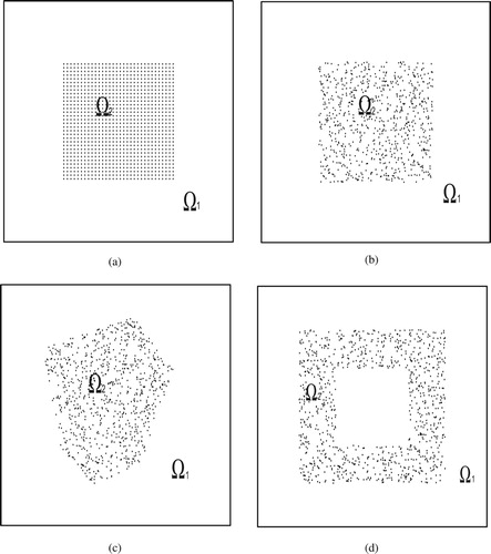
1. case 1: ${\mathrm{\Omega }}_1=[-\pi /2,\pi /2]\times [-\pi /2,\pi /2],$ and the nodes are equidistant (Figure 1(a)).

2. case 2: ${\mathrm{\Omega }}_1=[-\pi /2,\pi /2]\times [-\pi /2,\pi /2],$ and the nodes are random scatter (Figure 1(b)).

3. case 3: ${\mathrm{\Omega }}_1$ is a polygon with vertices at $(-2,-1.5)$, $(-1.5,-1.1)$, $(-0.6,-2.1)$, $(0.5,2.3)$, $(0.7,-1.5)$, $(1.6,0.9),$ and the nodes are random scatter (Figure 1(c)).

4. case 4: ${\mathrm{\Omega }}_1$ is a rectangular ring, and the nodes are random scatter (Figure 1(d)).

Figure 1. Domains and nodes for Example 4.1: (a) case 1, (b) case 2, (c) case 3, and (d) case 4.

Firstly, we observe that the impact of parameter q. The relative errors of Case 1 for various q are given in Table 1. The results show that the errors become smaller with the increase of q and the improvement becomes less obvious when q is lager than 32. So we test other cases with q = 32.

Table 1. The numerical results of Case 1 for Example 4.1.

	${\mathcal{E}}_1$					$\frac{{\mathcal{E}}_1}{{\delta }_1^{0.7}}$	${\mathcal{E}}_2$					$\frac{{\mathcal{E}}_2}{{\delta }_1^{0.5}}$
${\delta }_1$	q = 8	q = 16	q = 32	q = 64	q = 128	q = 32	q = 8	q = 16	q = 32	q = 64	q = 128	q = 32
1e−1	1.93e−1	1.26e−1	1.20e−1	1.24e−1	1.20e−1	6.05e−1	6.23e−1	4.77e−1	4.62e−1	4.75e−1	4.66e−1	1.46e+0
1e−2	5.86e−2	3.38e−2	2.73e−2	2.78e−2	2.77e−2	6.86e−1	3.83e−1	1.84e−1	1.39e−1	1.44e−1	1.44e−1	1.40e+0
1e−3	2.78e−2	7.89e−3	5.80e−3	5.78e−3	5.75e−3	7.30e−1	2.78e−1	6.46e−2	4.51e−2	4.40e−2	4.42e−2	1.43e+0
1e−4	2.25e−2	2.48e−3	1.30e−3	1.25e−3	1.26e−3	8.20e−1	2.54e−1	2.93e−2	1.42e−2	1.38e−2	1.41e−2	1.42e+0

The relative errors of Cases 2–4 are given in Table 2. Comparing the data of columns 2–3 in Table 2 with the ones of column 4 and column 10 in Table 1, we can see that the results of random scatter nodes are worse than the equidistant nodes. And from Table 2, we can see that the method works well for all cases.

Table 2. The numerical results of Case 2-4 with q = 32 for Example 4.1.

	Case 2				Case 3				Case 4
${\delta }_1$	${\mathcal{E}}_1$	${\mathcal{E}}_2$	$\frac{{\mathcal{E}}_1}{{\delta }_1^{0.5}}$	$\frac{{\mathcal{E}}_2}{{\delta }_1^{0.4}}$	${\mathcal{E}}_1$	${\mathcal{E}}_2$	$\frac{{\mathcal{E}}_1}{{\delta }_1^{0.7}}$	$\frac{{\mathcal{E}}_1}{{\delta }_1^{0.5}}$	${\mathcal{E}}_1$	${\mathcal{E}}_2$	$\frac{{\mathcal{E}}_1}{{\delta }_1^{0.7}}$	$\frac{{\mathcal{E}}_2}{{\delta }_1^{0.5}}$
1e−1	1.59e−1	5.13e−1	5.05e−1	1.29e+0	6.04e−2	3.92e−1	3.03e−1	1.24e+0	4.85e−2	1.56e−1	2.43e−1	4.93e−1
1e−2	5.44e−2	2.39e−1	5.44e−1	1.51e+0	9.00e−3	1.13e−1	2.26e−1	1.13e+0	1.14e−2	6.40e−2	2.86e−1	6.40e−1
1e−3	1.40e−2	7.41e−2	4.43e−1	1.17e+0	1.90e−3	3.56e−2	2.39e−1	1.13e+0	1.80e−3	1.54e−2	2.27e−1	4.87e−1
1e−4	4.50e−3	3.31e−2	4.50e−1	1.32e+0	5.60e−4	1.50e−2	3.53e−1	1.50e+0	3.20e−4	4.00e−3	2.02e−1	4.00e−1

The numbers in columns 7 and 13 in Table 1, and columns 4, 5, 8, 9, 12, 13 in Table 2 show that the ratios are stable when ${\delta }_1\to 0$. Moreover, fit the numbers in the above columns to (39) $k{\delta }_1^{{\omega }_i}={\mathcal{E}}_i,(i=1,2).$(39) (Find k and ${\omega }_i$, which can be determined by the data linearization method [36], so that $k{\delta }_1^{{\omega }_i}$ is the least-squares power curve.) We can get ${\omega }_1=0.6577,{\omega }_2=0.5030$ for case 1, ${\omega }_1=0.5241,{\omega }_2=0.4079$ for case 2, ${\omega }_1=0.6774,{\omega }_2=0.4751$ for case 3, ${\omega }_1=0.7343,{\omega }_2=0.5390$ for case 4 with q = 32.

From the above results, it can be seen that this method is suitable for several different node and region cases. We can also see that ${\omega }_i(i=1,2)$ in case 2 are worse than the other cases. The results may be caused by the discretization errors.

Now we present the results of two examples from [12,37]. The numerical processing of this method is simpler.

Example 4.2

[12]

Choose the exact function $f(x,y)=(2-(2x-1{)}^2{)}^2\cos (4y)$. Equation (14(14) $({\mathcal{F}}^{\ast }\mathcal{F}+\beta {\mathcal{D}}_q^2)\mathbf{v}={\mathcal{F}}^{\ast }{f}^{\delta }.$(14) ) is discretized by the collocation method, and the nodes $\overline{\mathbf{x}}$ are given as ${\mathrm{\Omega }}_1=[0,1]\times [0,\pi ]$ and are equidistant. We also create noisy data by adding some random errors to the exact values in manner of (37(37) $f^{\delta }(\overline{\mathbf{x}})=f(\overline{\mathbf{x}})+\text{randn}(\text{size}(\overline{\mathbf{x}}))\cdot {\delta }_1,$(37) ). The error is controlled by ${\delta }_1,$ and the numerical results are shown in Table 3 and Figures 2(a–c) and 3(a–c). We take $q=32,{\delta }_1={10}^{-3}$ in Figures 2 and 3.

Figure 2. The first-order derivative of $f(x,y)$ in Example 4.2 with q = 32 and ${\delta }_1={10}^{-3}$. (a) The exact function of $f_x+f_y$, (b) the constructed function of $f_x+f_y$, and (c) the constructed error function of $f_x+f_y$.

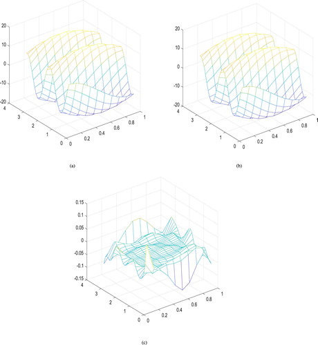
Figure 3. The second-order derivative of $f(x,y)$ in Example 4.2 with q = 32 and ${\delta }_1={10}^{-3}$. (a) The exact function of $f_{xx}+f_{xy}+f_{yy}$, (b) the constructed function of $f_{xx}+f_{xy}+f_{yy}$, and (c) the constructed error function of $f_{xx}+f_{xy}+f_{yy}$.

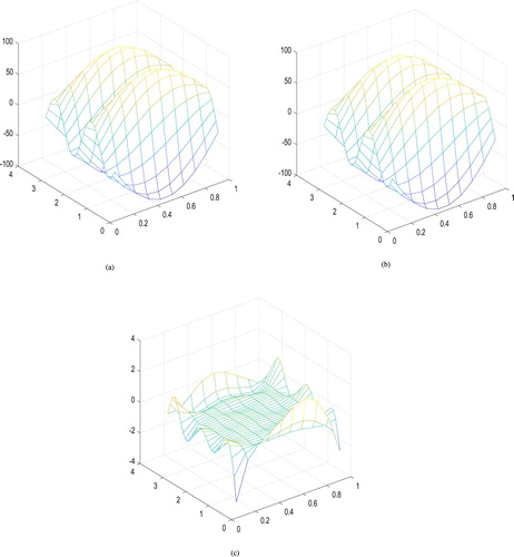
Table 3. The numerical results of Example 4.2.

	${\mathcal{E}}_1$					$\frac{{\mathcal{E}}_1}{{\delta }_1^{0.8}}$	${\mathcal{E}}_2$					$\frac{{\mathcal{E}}_2}{{\delta }_1^{0.7}}$
${\delta }_1$	q = 8	q = 16	q = 32	q = 64	q = 128	q = 32	q = 8	q = 16	q = 32	q = 64	q = 128	q = 32
1e−1	8.10e−2	5.48e−2	6.04e−2	1.13e−1	1.46e−1	3.81e−1	1.65e−1	1.22e−1	1.46e−1	4.39e−1	6.43e−1	7.33e−1
1e−2	2.11e−2	1.13e−2	1.27e−2	1.37e−2	1.72e−2	5.06e−1	7.99e−2	3.98e−2	4.96e−2	5.40e−2	8.05e−2	1.25e+0
1e−3	8.20e−3	3.10e−3	2.00e−3	1.80e−3	1.90e−3	5.02e−1	5.05e−2	1.68e−2	9.00e−3	7.20e−3	8.50e−3	1.33e+0
1e−4	5.60e−3	8.98e−4	2.80e−4	3.41e−4	3.55e−4	4.44e−1	4.24e−2	6.80e−3	1.50e−3	2.00e−3	2.20e−3	9.46e−1

Substitute the numbers in columns 7 and 13 in Table 3 into the right-hand side of the (39(39) $k{\delta }_1^{{\omega }_i}={\mathcal{E}}_i,(i=1,2).$(39) ), we can obtain ${\omega }_1=0.7804,{\omega }_2=0.6707$ with q = 32 for Example 4.2.

From the figures, we can see that the numerical results is quite good.

Example 4.3

[37]

Let $f(x,y)=\sin (\pi x)(\cos (2y)+0.5),(x,y)\in {\mathrm{\Omega }}_1$ where ${\mathrm{\Omega }}_1=\{(x,y)|\frac{1}{4}\le x\le \frac{3}{4},\frac{\pi }{2}\le y\le \frac{3\pi }{2}\}$ and the nodes are equidistant. Numerical results are shown in Table 4 and Figures 4(a–c) and 5(a–c). We take $q=32,{\delta }_1={10}^{-3}$ in Figures 4 and 5. And we give the cpu time denoted by T in Table 4 when q = 32 for ${\mathcal{E}}_1$ and ${\mathcal{E}}_2$.

Figure 4. The first-order derivative of $f(x,y)$ in Example 4.3 with q = 32 and ${\delta }_1={10}^{-3}$. (a) The exact function of $f_x+f_y$, (b) the constructed function of $f_x+f_y$, and (c) the constructed error function of $f_x+f_y$.

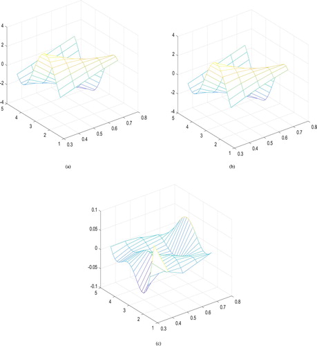
Figure 5. The second-order derivative of $f(x,y)$ in Example 4.3 with q = 32 and ${\delta }_1={10}^{-3}$. (a) The exact function of $f_{xx}+f_{xy}+f_{yy}$, (b) the constructed function of $f_{xx}+f_{xy}+f_{yy}$, and (c) the constructed error function of $f_{xx}+f_{xy}+f_{yy}$.

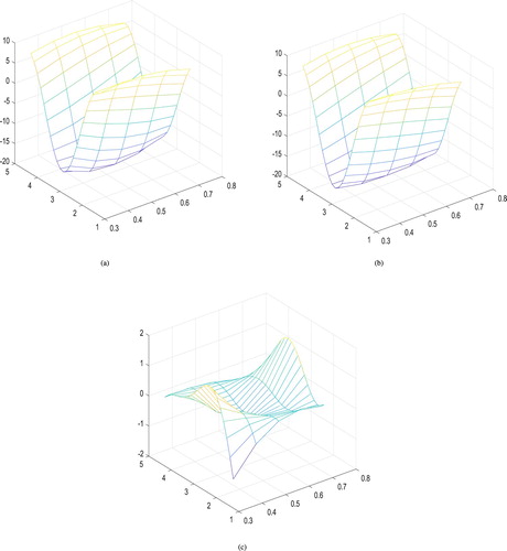
Table 4. The numerical results of Example 4.3

	${\mathcal{E}}_1$					$\frac{{\mathcal{E}}_1}{{\delta }_1^{0.7}}$	${\mathcal{E}}_2$					$\frac{{\mathcal{E}}_2}{{\delta }_1^{0.6}}$
${\delta }_1$	q = 8	q = 16	q = 32(T)	q = 64	q = 128	q = 32	q = 8	q = 16	q = 32(T)	q = 64	q = 128	q = 32
1e−1	2.78e−1	2.33e−1	2.19e−1 (26.29s)	6.10e−1	6.10e−1	0.110e−1	3.62e−1	3.05e−1	2.84e−1 (26.22s)	6.10e−1	6.10e−1	0.113e−1
1e−2	5.01e−2	5.48e−2	8.79e−2 (28.79s)	8.96e−2	8.90e−2	0.221e−1	9.49e−2	1.07e−1	2.14e−1 (28.50s)	8.96e−2	8.90e−2	0.339e−1
1e−3	1.65e−2	1.20e−2	1.38e−2 (27.97s)	1.47e−2	1.50e−2	0.174e−1	5.65e−2	4.10e−2	5.29e−2 (27.85s)	1.47e−2	1.50e−2	0.334e−1
1e−4	6.80e−3	2.20e−3	1.50e−3 (29.64s)	1.50e−3	1.50e−3	0.946e+0	3.39e−2	9.40e−3	5.60e−3 (29.69s)	1.50e−3	1.50e−3	0.141e−1

Substitute the numbers in columns 7 and 13 in Table 3 into the right-hand side of the (39(39) $k{\delta }_1^{{\omega }_i}={\mathcal{E}}_i,(i=1,2).$(39) ), we can get that ${\omega }_1=0.7300,{\omega }_2=0.5723$ with q = 32 for Example 4.3.

Compared with the results in [12,37], the performance of the method in this paper is satisfactory.

All the above examples are for infinitesimal differentiable functions. Now we give a less smooth function to test the validity of the method.

Example 4.4

Let (40) $f(x,y)=\cos 2\pi x\{\begin{array}{ll}-\frac{y^2}{2}& y\le 0\\ \frac{y^2}{2}& y\ge 0\end{array}$(40) $(x,y)\in {\mathrm{\Omega }}_1$, where ${\mathrm{\Omega }}_1=\{(x,y)|-1\le x\le 1,-1\le y\le 1\},$ and the nodes are equidistant. We take $f(x,y)$ as the unknown function to compute the numerical differentiation of its first-order derivatives. Numerical results are shown in Table 5 and Figure 6(a–c). We take $q=32,{\delta }_1={10}^{-3}$ in Figure 6 for ${\mathcal{E}}_1$.

Figure 6. The first-order derivative of $f(x,y)$ in Example 4.4 with q = 32 and ${\delta }_1={10}^{-3}$. (a) The exact function of $f_x+f_y$, (b) the constructed function of $f_x+f_y$, and (c) the constructed error function of $f_x+f_y$.

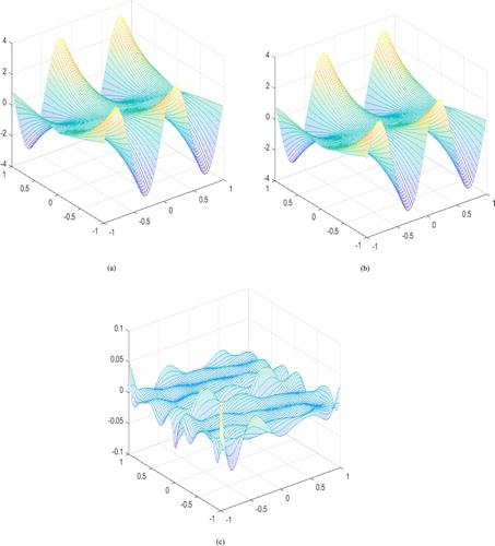
Table 5. The numerical results of Example 4.4.

	${\mathcal{E}}_1$					$\frac{{\mathcal{E}}_1}{{\delta }_1^{0.6}}$
${\delta }_1$	q = 8	q = 16	q = 32	q = 64	q = 128	q = 32
1e−1	2.31e−1	1.89e−1	2.08e−1	2.30e−1	2.38e−1	8.26e−1
1e−2	5.69e−2	3.84e−2	4.08e−2	4.40e−2	4.89e−2	6.47e−1
1e−3	6.90e−3	5.90e−3	6.50e−3	8.30e−3	8.50e−3	4.10e−1
1e−4	3.60e−3	3.80e−3	3.80e−3	3.60e−3	4.10e−3	9.55e−1

Substitute the numbers in columns 7 and 13 in Table 3 into the right-hand side of the (39(39) $k{\delta }_1^{{\omega }_i}={\mathcal{E}}_i,(i=1,2).$(39) ), we can obtain ${\omega }_1=0.6009$ with q = 32 for Example 4.4.

The reconstructed function are very similar to those of corresponding function. In general, we can see that our construction is effective. The above numerical results show that the proposed method is effective and promising for numerically computing the first- and second-order derivatives of functions with two variables from the noisy data.

5. Conclusions

A method based on Fourier extension has been proposed to obtain derivatives of two-dimensional functions. We have proved that the numerical method is stable. Numerical results for tests show that the method can work for any domain and the function with non-smooth derivatives. The method will be expected to deal with other ill-posed problem, which will be discussed in a future paper.

Disclosure statement

No potential conflict of interest was reported by the authors.

Additional information

Funding

This work was supported by the National Natural Science Foundation of China (No. 11201085, Q18306), Project of enhancing school with the innovation of Guangdong Ocean University (2016050202) and Class Discipline of Zhejiang-A (Zhejiang University of Finance and Economics-Statistics).

References

- Deans SR. The radon transform and some of its applications. New York: A Wiley-Interscience Publication; 1983.
- Egger H, Engl HW. Tikhonov regularization applied to the inverse problem of option pricing: convergence analysis and rates. Inverse Probl. 2005;21(3):1027–1045.
- Gorenflo R, Vessella S. Abel integral equations, analysis and applications. Berlin: Springer-Verlag; 1991. (Lecture Notes in Mathematics; vol. 1461).
- Hanke M, Scherzer O. Error analysis of an equation error method for the identification of the diffusion coefficient in a quasi-linear parabolic differential equation. SIAM J Appl Math. 1998;59(3):1012–1027.
- Wan XQ, Wang YB, Yamamoto M. Detection of irregular points by regularization in numerical differentiation and application to edge detection. Inverse Probl. 2006;22(3):1089–1103.
- Yin BB, Ye YZ. Recovering the local volatility in Black–Scholes model by numerical differentiation. Appl Anal. 2006;85(6–7):681–692.
- Cullum J. Numerical differentiation and regularization. SIAM J Numer Anal. 1971;8(2):254–265.
- Fu CL, Feng XL, Qian Z. Wavelets and high order numerical differentiation. Appl Math Model. 2010;34(10):3008–3021.
- Hanke M, Scherzer O. Inverse problems light: numerical differentiation. Am Math Mon. 2001;108:512–521.
- Hu B, Lu S. Numerical differentiation by a Tikhonov regularization method based on the discrete cosine transform. Appl Anal. 2012;91(4):719–736.
- Ramm A, Smirnova A. On stable numerical differentiation. Math Comput. 2001;70(235):1131–1153.
- Wang YB, Wei T. Numerical differentiation for two-dimensional scattered data. J Math Anal Appl. 2005;312(1):121–137.
- Wang YB, Jia XZ, Cheng J. A numerical differentiation method and its application to reconstruction of discontinuity. Inverse Probl. 2002;18(6):1461–1476.
- Wang ZW, Wen RS. Numerical differentiation for high orders by an integration method. J Comput Appl Math. 2010;234(3):941–948.
- Wei T, Hon YC. Numerical differentiation by radial basis functions approximation. Adv Comput Math. 2007;27(3):247–272.
- Xu HL, Liu JJ. Stable numerical differentiation for the second order derivatives. Adv Comput Math. 2010;33(4):431–447.
- Yang L. A perturbation method for numerical differentiation. Appl Math Comput. 2008;199(1):368–374.
- Zhao ZY. A truncated Legendre spectral method for solving numerical differentiation. Int J Comput Math. 2010;87(14):3209–3217.
- Zhao ZY, Meng ZH. Numerical differentiation for periodic functions. Inverse Probl Sci Eng. 2010;18(7):957–969.
- Zhao ZY, Meng ZH, He GQ. A new approach to numerical differentiation. J Comput Appl Math. 2009;232(2):227–239.
- Wei T, Hon YC, Wang YB. Reconstruction of numerical derivatives from scattered noisy data. Inverse Probl. 2005;21(2):657–672.
- Xie O, Zhao ZY. Numerical differentiation of 2d functions by a mollification method based on Legendre expansion. Int J Comput Sci. 2013;10(1):729–734.
- Zhao ZY, Meng ZH, Xu L, et al. A new mollification method for numerical differentiation of 2d periodic functions. International Joint Conference on Computational Sciences and Optimization, Cso 2009; April 24–26; Sanya, Hainan, China; 2009. p. 205–207.
- Ling L. Finding numerical derivatives for unstructured and noisy data by multiscale kernels. SIAM J Numer Anal. 2006;44(4):1780–1800.
- Adcock B, Huybrechs D, Martín-Vaquero J. On the numerical stability of Fourier extensions. Found Comput Math. 2014;14(4):635–687.
- Boyd JP. A comparison of numerical algorithms for Fourier extension of the first, second, and third kinds. J Comput Phys. 2002;178(1):118–160.
- Huybrechs D. On the Fourier extension of nonperiodic functions. SIAM J Numer Anal. 2010;47(6):4326–4355.
- Lyon M, Picard J. The Fourier approximation of smooth but non-periodic functions from unevenly spaced data. Adv Comput Math. 2014;40(5–6):1073–1092.
- Lyon M. A fast algorithm for Fourier continuation. SIAM J Sci Comput. 2011;33(6):3241–3260.
- Lyon M. Approximation error in regularized svd-based Fourier continuations. Appl Numer Math. 2012;62(12):1790–1803.
- Engl HW, Hanke M, Neubauer A. Regularization of inverse problems. Vol. 375. Dordrecht: Kluwer Academic Publishers; 2000.
- Nair MT, Pereverzev SV, Tautenhahn U. Regularization in Hilbert scales under general smoothing conditions. Inverse Probl. 2005;21(6):1851–1869.
- Adams RA. Sobolev spaces. New York (NY): Academic Press; 1975.
- Boyd JP. Fourier embedded domain methods: extending a function defined on an irregular region to a rectangle so that the extension is spatially periodic and C∞. Appl Math Comput. 2005;161(2):591–597.
- Boyd JP. Asymptotic Fourier coefficients for a C∞ bell (smoothed-top-hat) & the Fourier extension problem. J Sci Comput. 2006;29(1):1–24.
- Mathews JH, Fink KD. Numerical methods using MATLAB. 4th ed. Englewood Cliffs (NJ): Prentice-Hall; 2004.
- Nakamura G, Wang SZ, Wang YB. Numerical differentiation for the second order derivatives of functions of two variables. J Comput Appl Math. 2008;212(2):341–358.