Comparison of TVcDM and DDcTV algorithms in image reconstruction

ABSTRACT

The total variation (TV) minimization algorithms is a classical representative of the optimization algorithms and have been widely used for their simpleness, robustness, expandability and their potential of accurately reconstructing images from sparse data or noisy data. The commonly used constrained TV (cTV) program is the data-divergence constrained TV (DDcTV) minimization. The other recently proposed cTV program is the TV constrained data-divergence minimization (TVcDM). In the work, we compare the two programs the convergence rate and the reconstruction accuracy via the sparse-view projection set and the noisy projection set in the context of CT. Further, we compare their reconstruction accuracy via real data in electron paramagnetic resonance imaging (EPRI). The studies show that TVcDM has much faster convergence rate relative to DDcTV and that TVcDM may achieve higher accuracy in most cases no matter in sparse-view projections CT reconstructions or in noisy projections CT reconstructions or in EPRI sparse reconstructions. From a comprehensive perspective, TVcDM has superior convergence and accurate reconstruction performance relative to DDcTV and should be recommended in the application of TV reconstruction algorithms. The knowledge and insights gained in the work may be extended to the performance analysis of other optimization-based reconstruction algorithms.

KEYWORDS:

• Optimization-based reconstruction
• total variation minimization
• Chambolle–Pock algorithm
• constrained optimization
• image reconstruction

SUBJECT CLASSIFICATION CODE:

• 94A08

1. Introduction

Optimization-based image reconstruction algorithms have been systematically and deeply investigated in a variety of imaging modalities [1], including computed tomography (CT) [2], magnetic resonance imaging (MRI) [3–5] and electron paramagnetic resonance imaging (EPRI) [6]. Optimization-based algorithms may employ the compressed sensing (CS) theory [7] or partial separability theory [8] and achieve improved reconstruction quality. Total variation (TV) minimization algorithm is a classical CS-based reconstruction algorithm which may accurately reconstruct images from sparse data or noisy data [9]. From 2006 to 2008, Pan group at the University of Chicago proposed and improved a constrained TV (cTV) minimization algorithm and applied it to fan-beam and cone-beam CT, achieving accurate sparse reconstructions [10,11]. Since then, TV model has been widely and deeply investigated and improved [12]. TV model has been successfully applied to CBCT [13], offset-detector CBCT [14], short scan CBCT [15], C-arm CBCT [16], positron emission tomography (PET) [17] and EPRI [18]. TV model also has been extended and improved into numerous varietal TV models. The TpV model, with $p\in [0,1]$, may further promote sparsity for non-convex p quasi-norm is closer to ${\ell }_0$ norm than ${\ell }_1$ norm used in the classical TV model [19]. The high order TV model may suppress the possible stair-case effect [20]. The adaptive-weighted TV model may achieve higher accuracy in low-dose CT [21]. Huber TV may preserve image texture and edge [22]. Non-local TV model may better preserve image texture and fine structures [23]. The nuclear TV model may employ the relevant prior information among the multi-channel spectral CT images and may further improve the sparse reconstruction accuracy [24]. Though these varietal TV models exist, the classical TV model is still under deep exploration for it is simple, robust and easy to extend to high dimensional image reconstructions.

TV model consists of two terms: data fidelity term and TV regularization term. Suppose that the imaging model may be formulated as a linear system, shown in (1). According to the constraint form, there are three specific TV models, shown in (2), (3) and (4). (1) $\begin{array}{rl}g& =Au,\end{array}$(1) (2) $\begin{array}{rl}{u}^{\ast }& =\arg \underset{u}{min}\frac{1}{2}||g-Au|{|}_2^2+w||u|{|}_{\text{TV}},\end{array}$(2) (3) $\begin{array}{rl}{u}^{\ast }& =\arg \underset{u}{min}||u|{|}_{\text{TV}}\text{s}\text{.t}\text{.}||g-Au|{|}_2\le ϵ,\end{array}$(3) (4) $\begin{array}{rl}{u}^{\ast }& =\text{arg}\underset{u}{min}||g-Au|{|}_2^2\text{s.t.}||u|{|}_{TV}\le t_1,\end{array}$(4)

In (1), $g$ is a vector of size $M$, indicating the discrete data, $u$ a vector of size $N$, indicating the discrete image and $A$ a matrix of size $M\times N$, indicating the system matrix. For 2D parallel-beam CT, $A$ indicates the 2D Radon transform; for 2D fan-beam CT or 3D cone-beam CT, $A$ indicates the ray transform; for MRI, $A$ indicates the Fourier transform and for 3D EPRI, $A$ indicates the 3D Radon transform. For the linear system is usually large-scale, ill-posed and under-determined, the direct inversion of (1) is impossible. Thus, we further perform optimization programme modelling and design the three specific TV models shown in (2)–(4).

(2) is the unconstrained TV (ucTV) model. $\frac{1}{2}||g-Au|{|}_2^2$ is the data fidelity term and $||u|{|}_{\text{TV}}$ is the TV regularization term. $w$ is the model parameter which may balance the magnitude of data fidelity and TV regularization. It is commonly used for it is easy to solve [25,26]. However, $w$ has not clear physical meaning so that it is very hard to select. In addition, when $w$ is very small, the convergence rate will be very low [27].

(3) and (4) are two constrained TV (cTV) models. (3) is the data-divergence constrained TV (DDcTV) minimization model, whereas (4) is the TV constrained data-divergence minimization (TVcDM) model. In (3), $ϵ$ is the data tolerance, which indicates the noise level and system-inconsistence. For it has clear physical meaning, it may be determined by analysing the imaging system characteristics [28]. Recently, Pan group proposed the novel TVcDM model and applied it to CT [15] and PET [17]. In 2018, the first and second author of this paper worked together with Pan group and achieved accurate image reconstruction from sparse-view projections in EPRI by use of the TVcDM model [6]. One reason why we select TVcDM model is that the model parameter, $t_1$, is easy to tune for its impact on reconstruction is not so sensitive as the impact of data tolerance on DDcTV reconstruction.

DDcTV and TVcDM have different optimization sense. DDcTV selects the solution of the minimal TV value from the convex set defined by the data fidelity term, whereas TVcDM selects the solution of the maximal fidelity to the data from the convex set defined by the TV regularization term. Thus, the two models converge to the different solution with the imaging conditions the same. Additionally, we find the convergence rates of the two models are quite different.

Based on the preliminary theory analysis and our reconstruction practices, we systematically compare DDcTV and TVcDM models in the context of CT and EPRI in this paper. In CT reconstructions, the work uses two mathematical phantom, Shepp–Logan and FORBILD phantom, to perform studies to ensure the ground truth exists. First, we compare the convergence rates of the two models in the condition of inverse crime. Second, we compare the reconstruction accuracy of the two models via sparse-view projections and noisy projections to evaluate the sparse reconstruction and noisy projections reconstruction capabilities of the two models, respectively. In EPRI reconstruction, we use real data to compare the two models and evaluate their sparse reconstruction capability.

These TV models may be solved by many optimization algorithms such as adaptive steepest descent- projection onto convex sets (ASD-POCS) [11], alternating direction method of multipliers (ADMM) [25], split Bregman [26], and Chambolle–Pock (CP) algorithm [22,29,30]. The CP algorithm is used to solve the two models for it has some advantages relative to ASD-POCS and ADMM or split Bregman: first, it may solve all the convex optimization programmes, no matter it is smooth or not; second, all the algorithm parameters may be determined by fixed equations rather than artificially selections; third, each sub-problem has close form; forth, it has been mathematically proved to be convergent.

In Section 2, we introduce the DDcTV and TVcDM models and their corresponding CP algorithms. In Section 3, we compare the convergence rates of the two models. In Section 4, we compare the reconstruction accuracy of the two models via several sparse-view projection sets of different sparsity-level. In Section 5, several noisy projection sets of different noise level are used to evaluate the reconstruction accuracy of the two models. In Section 6, we compare the two models via real data in EPRI. Discussions and conclusion are given in Section 7.

2. Methods

In this section, we first describe the TV norm in the context of 2D CT, then introduce two balanced DDcTV and TVcDM models and give their CP algorithms, finally the reconstruction parameters, convergence metrics and reconstruction quality metrics are also illuminated. The TV norm for 3D EPRI may be obtained by simple 3D extension. The two CP algorithms are suitable not only for CT but also for EPRI.

2.1. TV norm

$||u|{|}_{\text{TV}}$, the TV norm of an image, may be defined as [15,16,31] (5) $||u|{|}_{\text{TV}}=||{|Du|}_{\text{mag}}|{|}_1,$(5) where $D$ is a matrix of size $2N\times N$, indicating the discrete gradient transform (DGM), and is of the form, (6) $D=\left(\begin{array}{c}{D}_1\\ D_2\end{array}\right)$(6) where $D_1$ and $D_2$ are both matrices of size $N\times N$, indicating the gradient transform along $x$ axis and $y$ axis, respectively.

Let $u_{x,y}$, $x\in [1,n_x],y\in [1,n_y]$ indicates a pixel of the 2D image, then $D_1$ transform may be indicated as (7) $(D_{1}u{)}_{x,y}=\{\begin{array}{ll}{u}_{x,y}-u_{x-1,y}& x\in [2,n_x]\\ 0& x=1\end{array}$(7)

and $D_2$ transform may be indicated as (8) $(D_{2}u{)}_{x,y}=\{\begin{array}{ll}{u}_{x,y}-u_{x,y-1}& y\in [2,n_y]\\ 0& y=1\end{array}$(8) $|\cdot {|}_{mag}$ is the magnitude of a 2D vector and may be defined with ${\ell }_1$ norm type or ${\ell }_2$ norm type. Here we use ${\ell }_2$ norm to define $|\cdot {|}_{mag}$ as (9) ${\left|\begin{array}{c}a\\ b\end{array}\right|}_{\text{mag}}=\left||\begin{array}{c}a\\ b\end{array}\right|{|}_2=\sqrt{a^2+b^2}$(9) thus $|Du{|}_{mag}$ is the isotropic gradient magnitude transform of an image. And the isotropic TV norm may be indicated as (10) $||u|{|}_{TV}=||{|Du|}_{\text{mag}}|{|}_1=\sum _{x,y}\sqrt{{{(D_{1}u)}_{x,y}}^2+{{(D_{2}u)}_{x,y}}^2}.$(10)

2.2. DDcTV model and its CP algorithm

First, we introduce a balanced DDcTV model other than the form in (3) by incorporating two balance parameters, $\lambda$ and $\nu$, into (3): (11) $u^{\ast }=\arg \underset{u}{min}\nu ||u|{|}_{\text{TV}},\text{s}.\text{t}.\lambda ||g-Au|{|}_2\le \lambda ϵ,$(11) where the function of $\lambda$ and $\nu$ is to balance the relative magnitude of the two terms, data fidelity term and TV regularization term. Our previous studies show that they cannot impact the solution of (3) but may impact the convergence rate of (3). Appropriate selected balance parameters may speed up the convergence rate of (3). This is the reason why we use the balanced DDcTV model.

Without showing the derivation of the CP algorithm instance of DDcTV model, we list the DDcTV-CP algorithm instance in Algorithm 1. The original DDcTV-CP algorithm derivation is in [30], from which one may learn the derivation method of CP algorithm instance.

Table

Algorithm 1. Pseudocode for N steps of the DDcTV-CP algorithm instance
INPUT:  $g$, $A$,$D$ $ϵ$; $\lambda$, $b$
1: ${\nu }_A=\frac{{||A||}_{sv}}{{||D||}_{sv}}$; $\nu =b{\nu }_A$
2: $L={\Vert \begin{array}{c}\lambda A\\ \nu D\end{array}\Vert }_{sv}$; $\sigma =\frac{1}{L},\tau =\frac{1}{L}$, $\theta =1,n=0$
3: $u_0=0;p_0=0;q_0=0;{\overline{u}}_0=0$
4: Repeat
5: $a=p_n+\sigma \lambda (A{\overline{u}}_n-g)$
6: $p_{n+1}=\text{max}({||a||}_2-\sigma \lambda ϵ,0)\times a/||a|{|}_2$
7: $\text{c}=q_n+\sigma \nu \text{D}{\overline{u}}_n$
8: $q_{n+1}=c/max(1_I,{|c|}_{\text{mag}})$
9: $u_{n+1}=u_n-\tau \lambda A^T{p}_{n+1}-\tau \nu D^T{q}_{n+1}$
10: ${\overline{u}}_{n+1}=u_{n+1}+\theta (u_{n+1}-u_n)$
11: $n=n+1$
12: Until  $n\ge N$
OUTPUT: The designed solution $u_N$.

In Algorithm 1, $u,\overline{u}\in R^N$, $p,a\in R^M$, $q,c\in R^{2N}$. In line 8, $1_I\in R^N$ is a ‘1’ vector in image space $I=R^N$. In line 2, the calculation algorithm of $L$ is shown in Algorithm 2 [30].

Table

Algorithm 2. Pseudocode for N steps of the generic power method to calculate L
1: $x_0=1;n=0$
2: Repeat
3: $x_{n+1}={\lambda }^2{A}^{T}A{x}_n+{\nu }^2{D}^{T}D{x}_n$
4: $x_{n+1}=x_{n+1}/||x_{n+1}|{|}_2$
5: $L={\Vert \begin{array}{c}\lambda A{x}_{n+1}\\ \nu D{x}_{n+1}\end{array}\Vert }_2$
6: $n=n+1$
7: Until  $n\ge N$

2.3. TVcDM model and its CP algorithm

Similar to the balanced DDcTV model, we introduce a balanced TVcDM model by incorporating two balance parameters, $\lambda$ and $\nu$, into (4): (12) $u^{\ast }=\text{argmin}\frac{\lambda }{2}||g-Au|{|}_2^2\text{s}\text{.t}\text{.}\nu ||u|{|}_{TV}\le \nu t_1.$(12)

We show the TVcDM-CP algorithm instance directly in Algorithm 3. The readers who are interested in the derivation details may refer to the Appendix of [16].

Table

Algorithm 3. Pseudocode for N steps of the TVcDM-CP algorithm instance
INPUT:  $g$, $A$,$D$, $t_1$; $\lambda$, $b$
1: ${\nu }_A=\frac{{||A||}_{SV}}{{||D||}_{SV}},\nu =b{\nu }_A$
2: $L={\Vert \begin{array}{c}A\\ \nu D\end{array}\Vert }_{SV}$; $\sigma =\frac{1}{L};\tau =\frac{1}{L};\theta =1;n=0$
3: $u_0=0;{\overline{u}}_0=0;p_0=0;q_0=0$
4: Repeat
5: $p_{n+1}=(p_n+\sigma (A{\overline{u}}_n-g))/(1+\sigma /\lambda )$
6.1:   $a=q_n+\sigma \nu D{\overline{u}}_n$
6.2:   $s=\text{ProjectOnto}{\ell }_1\text{Bal}{\text{l}}_{\nu t_1}(|a{|}_{mag}/\sigma )$
6.3:   $q_{n+1}=a(1_I-\sigma s/{|a|}_{mag})$
7: $u_{n+1}=u_n-\tau (A^T{p}_{n+1}+\nu D^T{q}_{n+1})$
8: ${\overline{u}}_{n+1}=u_{n+1}+\theta (u_{n+1}-u_n)$
9: $n=n+1$
10:  Until  $n\ge N$
OUTPUT: The designed solution $u_N$

In Algorithm 3, $u,\overline{u},\text{ s }\in R^N$, $p\in R^M$, $q,a\in R^{2N}$. In line 6.3, $1_I\in R^N$ is a ‘1’ vector in image space $I=R^N$. In line 2, the calculation algorithm of $L$ is shown in Algorithm 2. In line 6.2, $\text{ProjectOnto}{\ell }_1\text{Ball}$ is an operator which may project a vector to a ${\ell }_1$ ball of a specific radius. Its algorithm is shown in Algorithm 4.

Table

Algorithm 4. Pseudocode for $\text{ProjectOnto}{\ell }_1\text{Bal}{\text{l}}_a(x)$
1: if $||x_1||\le a$ then
2:    return $x$
3: end if
4: $m=|x|$
5: Sort $m$ in descending order
6: $k=max(j)\text{such}\text{that}{m}_j-\frac{1}{j}\left(\sum _{i=1}^j{m}_i-a\right)>0\text{for}\text{all}j\in [1,N]$
7: $\theta =(1/k)\left(\sum _{i=1}^k{m}_i-a\right)$
8: $w=\text{max}\text{(}|x|-\theta ,0\text{)}$
9: return $w\cdot \text{sign}(x)$

In Algorithm 4, $x$ is a vector of size $N$, $a$ is the radius of the ${\ell }_1$ ball. In line 4, $|\cdot |$ indicates calculating the absolute value in a componentwise manner. In line 9, ‘sign’ is the standard sign function: the function value for positive number is 1; for 0 is 0; and for negative number is −1.

2.4. Reconstruction parameters

Whether for DDcTV-CP or for TVcDM-CP algorithm, there are numerous parameters in the reconstruction algorithm. The parameters may be divided into two types: model parameters and algorithm parameters. The model parameters are those parameters which may impact the solution of the optimization model. The algorithm parameters are those parameters which do not impact the solution of the optimization model but may impact the convergence rate of the model-solving algorithm.

For DDcTV model, the model parameters include (1) calculation method of the system matrix, (2) the size of pixel, and (3) data tolerance. In the work, we use the accurate pixel-driven projection method to calculate the system matrix [32]. In the work, the pixel size is 1 which is the same with the length of the detector bin. The data tolerance, $ϵ$, has important impact on the solution of the optimization model. A specific data tolerance corresponds to a specific solution if other model parameters fixed. The previous studies show that too large $ϵ$ leads to too smooth image, whereas too small $ϵ$ leads to too noisy image. The best trade-off leads to the most accurate image for $ϵ$ at the balance-point may accurately describe the noise level and the system-inconsistence. According to the knowledge, we may select the optimal data tolerance in each DDcTV reconstruction. In the DDcTV-CP algorithm, the algorithm parameters include $\lambda ,\nu ,\sigma ,\tau \text{and}\theta$. $\sigma ,\tau \text{and}\theta$ are the inherent parameters in CP algorithm and may be determined by the equations in line 2 of Algorithm 1. $\lambda \text{and }\nu$ are the balance parameters introduced in (11). They may impact the convergence rate of the CP algorithm. We my select the optimal values for them by running CP algorithm with different combination values. In the work, we use $\lambda =1\text{and}\nu =0.1{\nu }_A$ for most cases to achieve high speed convergence.

For TVcDM model, the model parameters also include calculation method of system matrix and pixel size. Their determination methods are the same with those methods in DDcTV model. Another important model parameter in TVcDM model is the TV bound, $t_1$. Our previous study has shown that too large $t_1$ leads to too noisy image, whereas too small $t_1$ leads to too smooth image [6]. The best trade-off leads to the most accurate image for $t_1$ at the balance-point may accurately describe the TV value of the reconstructed image. In the TVcDM-CP algorithm, the algorithm parameters include $\lambda ,\nu ,\sigma ,\tau \text{and}\theta$. Their determination methods are the same with those methods in DDcTV-CP algorithm.

2.5. Metrics for practical convergence conditions

The DDcTV- and TVcDM-CP algorithm may achieve the ideal convergence only when the iteration number tends to infinite. Thus, it is necessary for us to design practical convergence conditions. In the work, we design three metrics for devising practical convergence conditions: dNDE (differential normalized data error), dNOE (differential normalized object error) and NTVE (normalized TV error), defined by (13) $\begin{array}{rl}dNDE(u_n)& =(||g-A{u}_n|{|}_2-||g-A{u}_{n-1}|{|}_2)/||g|{|}_2,\end{array}$(13) (14) $\begin{array}{rl}\text{dNOE}(u_n)& =(||u_n-u_{\text{truth}}|{|}_2-||u_{n-1}-u_{\text{truth}}|{|}_2)/||u_{\text{truth}}|{|}_2,\end{array}$(14) (15) $\begin{array}{rl}\text{dNTVE}(u_n)& =|({||u_n||}_{\text{TV}}-{||u_{n-1}||}_{\text{TV}})|/||u_n|{|}_{\text{TV}},\end{array}$(15) where $u_{truth}$ is the truth image, which exists in simulation studies employed in this work. When the three metrics all become small enough, the practical convergence conditions are achieved.

2.6. Metric for image quality evaluation

To quantitatively evaluate the reconstruction quality, we use RMSE (root mean square error) defined as (16) $\text{RMSE}(u_{\text{conv}})=||u_{\text{conv}}-u_{\text{truth}}|{|}_2/\sqrt{N},$(16) where $u_{\text{conv}}$ is the convergent solution and $u_{\text{truth}}$ is the truth image.

3. Comparison of convergence rate

To verify the correctness of an optimization-based image reconstruction algorithm, the inverse crime study is necessary. Inverse crime is a method to test if an inverse problem may be correctly and accurately solved. For DDcTV and TVcDM, the whole design chain includes imaging system modelling, optimization model modelling, solving algorithm design and computer implementation. To verify the correctness of the whole chain, we perform inverse crime studies for DDcTV-CP and TVcDM-CP algorithms. We use the Shepp–Logan and FORBILD phantoms to perform studies. The projection set is generated by the use of (1), therefore the linear system is absolutely consistent. If the projection set includes enough and ideal projections, then the two algorithms should accurately reconstruct the phantoms, indicating inverse crime succeeds.

In the meantime, we compare the convergence rate of DDcTV-CP and TVcDM-CP algorithms to direct the selection of the two models in cTV-based image reconstruction.

3.1. Imaging conditions and parameters determination

The size of the Shepp–Logan and FORBILD phantom are both $[256,256]$ and the pixel size is 1. The origin of the imaging coordinate system is located at pixel $[128,128]$. 60 projections in the angle range of $[0,\pi ]$ are evenly collected and each projection has 256 detector bins with the length of each bin being 1. The system matrix $A$ is calculated by use of the accurate pixel-driven projection method [32]. The projections are calculated by use of (1). Thus the projection data is of size $[256,60]$.

For DDcTV-CP, the model parameter $ϵ$ is set as 0 for there is not noise in the projections. Set $\lambda =1\text{and }\nu =0.1{\nu }_A$ to get fast convergence. For TVcDM-CP, the model parameter $t_1$ is set as ${u_{\text{truth}}}_{\text{TV}}$ for the existence of truth TV. Set $\lambda =1\text{ and}\nu =0.1{\nu }_A$, which is the same as those values designed in DDcTV-CP algorithm, to get fast convergence and obtain objective convergence-rate comparison under the same conditions with DDcTV-CP algorithm. The other algorithm parameters are determined according to the equations in Algorithm 1 and 3.

For this is inverse crime reconstruction, the convergence conditions for both models are set as $\text{RMSE}(u_{\text{conv}})\le 5\times {10}^{-4}$.

3.2. Inverse crime results

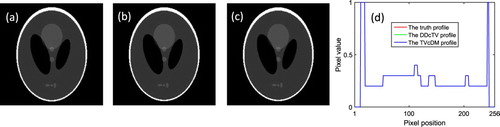
For Shepp–Logan reconstruction, DDcTV-CP stops at iteration 4221, whereas TVcDM-CP stops at iteration 857. The reconstructed images are shown in Figure 1. By visual inspection to (a)-(c), we may see that the three images are almost the same. From (d), it may be seen that the two reconstructed profiles are almost completely overlapped. At convergence point, the RMSE of the DDcTV-CP and TVcDM-CP images are both lower than $5\times {10}^{-4}$. Both the quantitative evaluation and qualitative visual inspection show that the inverse crime may be achieved by the two reconstruction algorithms.

Figure 1. The reconstructed Shepp–Logan images of DDcTV-CP and TVcDM-CP algorithms. (a) is the truth image; (b) and (c) are the images reconstructed by the DDcTV-CP and TVcDM-CP algorithms, respectively. (d) shows the profiles at the vertical center-line of the truth image and the reconstructed images by the two algorithms.

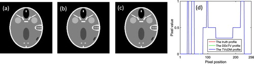
For FORBILD reconstruction, DDcTV-CP stops at iteration 7881, whereas TVcDM-CP stops at iteration 853. The reconstructed images are shown in Figure 2. At convergence point, the RMSE of the DDcTV-CP and TVcDM-CP images are both lower than $5\times {10}^{-4}$. Both the quantitative evaluation and qualitative visual inspection from Figure 2(a)–(d) show that the inverse crime may be achieved by the two reconstruction algorithms.

Figure 2. The reconstructed FORBILD images of DDcTV-CP and TVcDM-CP algorithms. The configuration pattern of subfigure (a)–(d) are the same with that in Figure 1.

3.3. Comparison of convergence rate

In the inverse crime reconstructions using the two algorithms, we have found that TVcDM is much faster than DDcTV. To observe the convergence behaviour of the two algorithms, we design two metrics and observe their iteration curve. One is $\text{RMSE}(u_n)$ and the other is $\text{DE}(u_n)$, defined in (17) and (18). $\text{RMSE}(u_n)$ measures the error of the reconstructed image relative to the truth image. $\text{DE}(u_n)$ measures the error of the generated projection relative to the original projection data. (17) $\begin{array}{rl}\text{RMSE}(u_n)& =||u_n-u_{\text{truth}}|{|}_2/\sqrt{N},\end{array}$(17) (18) $\begin{array}{rl}DE(u_n)& =||g-A{u}_n|{|}_2,\end{array}$(18)

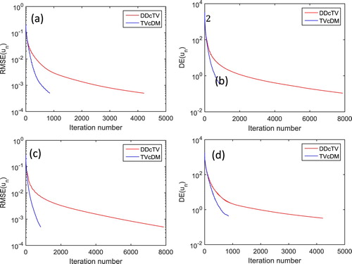
Figure 3 shows the iteration trend of $\text{RMSE}(u_n)$ and $\text{DE}(u_n)$ of the Shepp–Logan phantom and FORBILD phantom reconstructions. From the figure, it may be seen that the convergence rate of TVcDM is much faster than DDcTV. For the Shepp–Logan reconstruction, TVcDM needs 857 iterations, whereas DDcTV needs 4221 iterations. TVcDM is $(4221-857/857)\approx 3.9$ times faster than DDcTV. For the FORBILD reconstruction, TVcDM needs 853 iterations, whereas DDcTV needs 7881 iterations, so TVcDM is about 8.2 times faster than DDcTV. The acceleration ratio of FORBILD reconstruction is higher than that of the Shepp–Logan reconstruction, indicating that the acceleration ratio may increase with the increase of the complexity of the reconstructed image.

Figure 3. The iteration trend of DDcTV- and TVcDM-CP algorithms. (a) and (b) are for the Shepp–Logan reconstruction, whereas (c) and (d) are for the FORBILD reconstruction. (a) and (c) show the iteration trend of $\text{RMSE}(u_n)$, whereas (b) and (d) show the iteration trend of $\text{DE}(u_n)$.

Through the comparison of convergence rates of the two algorithms under inverse crime study, it appears that TVcDM-CP algorithm has a faster convergence rate relative to DDcTV-CP algorithm.

4. Comparison of sparse reconstruction capability

TV minimization algorithm may achieve accurate reconstruction from sparse-view projections for it embodies the core idea of compressed sensing. DDcTV and TVcDM both belong to the TV minimization category, so they both have capability to achieve accurate sparse reconstruction. However, their properties are quite different. DDcTV selects the solution with the minimal TV value from the convex set defined by the data-divergence term, whereas TVcDM selects the solution with the minimal data-divergence value from the convex set defined by the TV term. In sparse reconstruction, the image degradation law of the two models should be different. If the projection-view is too sparse, DDcTV tends to converge to a too smooth image of very low TV value, whereas TVcDM tends to converge to artefacts-terminated image for maintaining the TV value to be $t_1$. With the increase of projection number from too sparse case, the reconstruction quality will be better and better. However, the two models may have different accuracy for the difference in optimization sense. In the section, we use the Shepp–Logan and FORBILD phantoms to perform sparse reconstructions.

The imaging conditions and parameters determination are the same with that in Section 3.1 except that the projection number changes from 10 to 50 with a step-size of 10. The convergence conditions of the two algorithms both are (19) $\begin{array}{rl}\text{dNDE}(u_n)& \le {10}^{-4},\end{array}$(19) (20) $\begin{array}{rl}\text{dNOE}(u_n)& \le {10}^{-4},\end{array}$(20) (21) $\begin{array}{rl}\text{dNTVE}(u_n)& \le {10}^{-4}.\end{array}$(21)

Figure 4 shows the reconstructed Shepp–Logan images and Figure 5 (a) shows the curve of RMSE of the reconstructed image as a function of projection number. It may be seen from Figure 4 that the reconstructed images from projections of number more than or equal to 20 may achieve high quality reconstructions. The reconstructed images of DDcTV and TVcDM from 10 projections are both unacceptable. However, their properties are different: the DDcTV image from 10 projections is too smooth, whereas the TVcDM image from 10 projections suffers from streak artefacts. From Figure 5 (a), we see that the RMSEs of TVcDM images in most cases, including cases using 20, 30, 40 and 50 projections, are less than RMSEs of DDcTV images, indicating that TVcDM may achieve higher accuracy than DDcTV.

Figure 6 shows the reconstructed FORBILD images and Figure 5 (b) shows the curve of RMSE of the reconstructed image as the function of projection number. The two figures show that TVcDM may achieve higher accuracy than DDcTV in most cases including cases using 30, 40 and 50 projections and that DDcTV tends to too smooth, whereas TVcDM tends to too much artefacts if too sparse projections used.

Figure 4. The reconstructed Shepp–Logan images of DDcTV- (the first row) and TVcDM-CP (the second row) algorithms from 10, 20, 30, 40 and 50 projections uniformly collected in the range of $[0,\pi ]$.

Figure 5. Plots of RMSE of the reconstructed image as function of projection number. (a) and (b) are for the Shepp–Logan and FORBILD reconstructions, respectively.

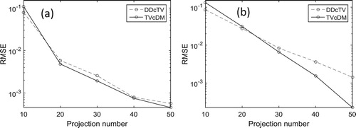
Figure 6. The reconstructed FORBILD images of DDcTV- (the first row) and TVcDM-CP (the second row) algorithms from 10, 20, 30, 40 and 50 projections uniformly collected in the range of $[0,\pi ]$.

5. Capability comparison of reconstructions from noisy projections

It is known that TV minimization may achieve high quality reconstructions not only from sparse-view projections but also noisy projections. In CT, the two cases correspond to the two strategies of low-dose CT: (1) reconstructions form sparse but high quality projections and (2) reconstructions from dense but noisy projections. The reason why TV minimization is competent for sparse reconstruction is TV minimization is one of the compressed sensing algorithm, whereas the reason why TV minimization may achieve high quality reconstruction from noisy projections is that TV minimization is a superior edge-preserving denosing method [33]. In the section, we use the Shepp–Logan and FORBILD phantoms to compare the reconstruction capabilities of DDcTV and TVcDM algorithms in the context of noisy projections.

The imaging conditions and parameters determination are the same with that in Section 3.1 except that projection number is 30 and the signal to noise ratio (SNR) of the projections changes from 30db to 50db with a step-size of 5db. For DDcTV, the model parameter $ϵ$ may be defined as the ${\ell }_2$ norm of the difference between the simulated projection data and the noisy projection data, i.e. $ϵ=||g_{\text{noise}}-g|{|}_2$. For TVcDM, the model parameter $t_1$ is set as $||u_{\text{truth}}|{|}_{\text{TV}}$ for the existence of truth TV. Figure 7 shows the reconstructed Shepp–Logan images of DDcTV and TVcDM algorithms from noisy projections. Figure 8 (a) shows the plot of RMSEs of the reconstructed images as a function of SNR.

Figure 7. The reconstructed Shepp–Logan images of DDcTV- (the first row) and TVcDM-CP (the second row) algorithms from projection data of SNR of 30db, 35db, 40db, 45db and 50db.

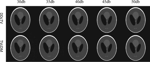
Figure 8. Plots of RMSEs of the reconstructed images as function of SNR in DDcTV and TVcDM reconstructions. (a) is for the Shepp–Logan phantom reconstruction. (b) is for the FORBILD phantom reconstruction.

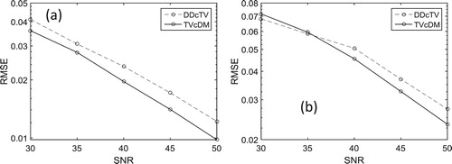
From Figure 7, we may see that the two algorithms both have accurate reconstruction capability if the SNR of the projection data is higher than or equal to 45db. With the decrease of SNR, the reconstructed images begin to degenerate for both DDcTV and TVcDM. But we note that the degeneration law of the two algorithms is different. DDcTV tends to too smooth image with the decrease of SNR, whereas TVcDM tends to too noisy image with the decrease of SNR. Figure 8 (a) shows that the TVcDM algorithm may achieve higher reconstruction accuracy than the DDcTV algorithm for every case of a specific SNR.

Figure 9 shows the reconstructed FORBILD images of DDcTV and TVcDM algorithms from noisy projections. Figure 8 (b) shows the plots of RMSEs of the reconstructed FORBILD images as a function of SNR.

Figure 9. The reconstructed FORBILD images of DDcTV- (the first row) and TVcDM-CP (the second row) algorithms from projection data of SNR of 30db, 35db, 40db, 45db and 50db.

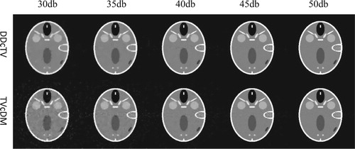
Figure 9 and Figure 8 (b) show that the TVcDM algorithm may achieve higher reconstruction accuracy than the DDcTV algorithm for most cases including cases of SNR of 40, 45 and 50db. And they show that the degradation law of DDcTV is that it tends to too smooth image, whereas the degradation law of TVcDM is that it tends to too noisy image.

6. Capability comparison of reconstructions from sparse-view projections in EPRI via real data

For three dimensional (3D) pulsed EPRI, the data is regarded as the projection data. A one dimensional projection signal at a specific angle may be obtained by inverse Fourier transform of the EPR signal at that angle. All projection signals in the full angle range make up the 3D Radon transform of the imaged object [34]. Image reconstruction for 3D EPRI is, in essence, to reconstruct the object from its projections via 3D inverse Radon transform.

We may design the DDcTV and TVcDM models and their CP algorithms for EPRI. The main differences in the models between 2D CT and 3D EPRI are the system matrix and the TV norm. The system matrix of EPRI indicates the 3D Radon transform and the TV norm is the ${\ell }_2$ norm of the discrete gradient transform of the 3D object.

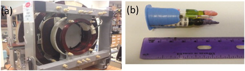
In the study, we collected data from a complex physical phantom by using a 250-MHz-pulse EPRI scanner (shown in Figure 10 (a)), controlled by SpecMan4EPR v2.1 [35], which was developed for EPR imaging in vivo physiology at The University of Chicago [36]. The complex physical phantom consists of three bottles and three tubes shown in Figure 10 (b), and each bottle/tube is filled with solution with different levels of spin probe concentration.

Figure 10. A prototype EPR imager (a) and a complex physical phantom consisting of three bottles and three tubes (b).

In the study, we collect 828 projections distributed uniformly in the angle range and refer to this projection set as full data set. At each angle, the spatial projection signal is obtained by inverse FFT of the EPR signal. Collecting 828 projections needs about 11 min, which is too long. To speed up the scan process, one effective approach is to collect projections from sparse views. To evaluate the sparse reconstruction capability of the two models, we use the data set of 100, 200, 300, 400 and 828 projections to perform reconstructions.

The length of each projection is 7 cm. The sampling interval of the projection signal is 0.0875 cm, so there are 80 measurements on each projection. The number of projections is 100, 200, 300, 400 and 828 projections, respectively, for the five different data sets. We reconstruct images of size 80×80×80 with voxel size being 0.0875cm×0.0875cm×0.0875 cm.

We use visual inspection and quantitative analysis to evaluate the reconstruction quality. Figures 11–13 show the x = 31, y = 48 and z = 48 slice images of the complex physical phantom, respectively. Figure 14 shows the plots of normalized RMSE as function of the number of projections.

Figure 11. The $\mathit{x}=31$ slice images of the reconstructed complex phantom. The number above the images indicates the projection number. The text on the left of the images indicates the used reconstruction algorithm. The display window is [0, 0.004].

Figure 12. The $\mathit{y}=48$ slice images of the reconstructed complex phantom. The meaning of the text and display window are the same with those in Figure 11.

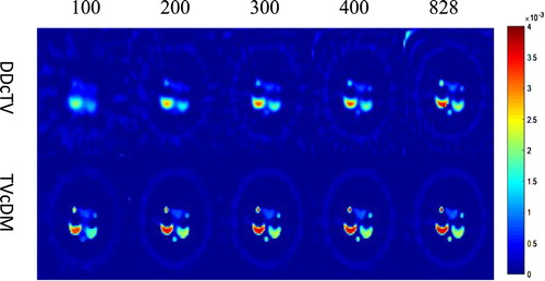
Figure 13. The $z=48$ slice images of the reconstructed complex phantom.

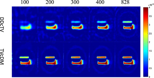
Figure 14. Plot of the normalized RMSE of the reconstructed images as function of projection number. The red line is for DDcTV, whereas the blue line is for TVcDM (colour online, B/W in print).

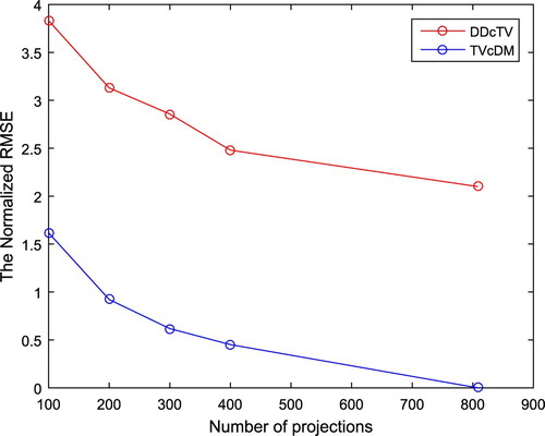
From Figures 11–13, we may see that TVcDM model may always achieve higher accuracy than DDcTV model. The DDcTV images are always too smooth. Maybe this is because DDcTV selects the image with the minimal TV from the convex set determined by the data fidelity term. For cases of projection number 100, 200, 300 and 400, the DDcTV images are all too smooth for their TV values are too low. Conversely, TVcDM images always have a fixed TV value, $t_1$, which may determine the smoothness of the reconstructed images. From Figure 12, it may be seen that the sharp bottle structure in the TVcDM images are clear, whereas the sharp structure in the DDcTV images may just be seen in the cases of projection number 400 and 828. The quantitative evaluation by the comparison of the normalized RMSE shown in Figure 14 has the consistent conclusion with the qualitative evaluation above.

In fact, this is why we selected TVcDM-CP algorithm as our standard optimization-based algorithm for sparse reconstruction and noisy projection reconstruction in EPRI [6,37]. In the section, our aim is to compare the two models in EPRI, so we do not show all the details on EPRI. The readers who want to know more detailed knowledge on EPRI are referred to [6,37].

7. Discussion and conclusions

We have compared the convergence rates and reconstruction accuracy of DDcTV-CP and TVcDM-CP algorithm. TVcDM has much faster convergence rate than DDcTV and has higher reconstruction accuracy in most cases no matter from sparse-view projections or from noisy projections, no matter for CT or for EPRI. For sparse reconstruction, DDcTV tends to too smooth image with the decrease of projection number, whereas TVcDM tends to an image of too much streak artefacts. For noisy-projections reconstruction, DDcTV tends to too smooth image with the decrease of SNR, whereas TVcDM tends to too noisy image.

Though we cannot mathematically prove that TVcDM should have a faster convergence rate than DDcTV, we may try to give some qualitative explanation. The constrained optimization problem means selecting a solution of minimal objective function value from the convex set defined by the constraint term. The constraint term of DDcTV is the data fidelity term, whereas that of TVcDM is the TV regularization term. TVcDM model means we know or we may guess the TV value of the reconstructed image. It is a reasonable deduction that we may fast find the reconstructed image if we have known its TV value. This is why TVcDM is much faster than DDcTV.

In sparse reconstructions, the DDcTV-CP algorithm tends to a too smooth image if the projection-view is too sparse. According to the compressed sensing theory, the accurate reconstruction of TV model needs to satisfy the ‘exact reconstruction principle (ERP)’, i.e. the number of measurements should be more than or equal to twice of the number of non-zero pixels in the gradient magnitude image [10]. Though the ERP is hard to evaluate in the imaging configurations other than ideal parallel-beam 2D reconstruction, it is certain that the sparse-level has a limit. In the sparse reconstructions of the work, the accurate reconstruction cannot be achieved if the projections are too sparse. When projections are too sparse, the convex set defined by the data fidelity term will be too large. In the too large convex set, the solution of DDcTV will have too small TV value, which means the solution-image will be too smooth. Conversely, the TVcDM-CP algorithm tends to an image of severe streak artefacts if the projection-view is too sparse. This is because the constraint term of the model is the TV regularization term. The TV value of the solution-image of minimal data divergence is always $t_1$, the TV bound defined in the TVcDM model.

In noisy projections reconstructions, the DDcTV-CP algorithm tends to a too smooth image, whereas the TVcDM-CP algorithm tends to a too noisy image if the projections are too noisy. This phenomenon may be qualitatively explained by the so-called $ϵ\text{ - ellipse}$ proposed by Pan group at the University of Chicago [11].

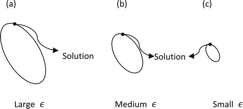
Figure 15 uses three ellipses to indicate three convex sets of different size corresponding to different noise levels. If the noise level is low, then the convex set defined by the data fidelity term is small (see Figure 15(c)). In the convex set, the solution of the minimal TV value may be accurate enough for it may suppress the noise by the TV regularization and the control of $ϵ$ value. With the increase of noise, the ellipse will be larger and larger (see Figure 15(b) and (a)), the solution of the minimal TV value tends to an image of smaller TV value than the truth image for the ellipse is so large that the solution freedom degree is very high. If the projections are too noisy, then the ellipse will be very large, i.e. the solution freedom degree will be very high. Selecting a solution of minimal TV value from the very large convex will lead to an image of too small TV value, which usually means the corresponding image is too smooth.

Figure 15. The schematic diagram of DDcTV-CP reconstructions from noisy projections. The ellipses, i.e. the $ϵ-\text{ellipse}$, indicate the convex sets defined by the data fidelities. Large, medium and small ellipse correspond to large, medium and small noise level. The black points on the ellipses indicate the solutions of DDcTV-CP algorithms.

However, TVcDM-CP always select a solution of minimal data divergence from the convex set defined by the TV term, i.e. the TV value of the reconstructed image is always the TV bound. Just because the TV value of the reconstructed image is fixed, it will not tend to smooth with the increase of the noisy level. However, if the projections are too noisy, the reconstructed image will appear too noisy even if the TV value is true because of the too noisy projections.

In conclusion, DDcTV-CP always tends to find a solution of small TV value, whereas TVcDM-CP always tends to find a solution of fixed TV value. Their degradation law with the decrease of projection number or increase of noise level is different: DDcTV tends to a smooth image, whereas TVcDM tends to an image of fixed TV value.

By the comparisons of DDcTV-CP and TVcDM-CP algorithms, we have found that TVcDM has faster convergence rate than DDcTV and that TVcDM may achieve higher reconstruction accuracy than DDcTV no matter in sparse reconstruction or noisy projections reconstruction. The investigation suggests one use TVcDM-CP algorithm in the constrained TV minimization reconstructions. The TV model has many variant models, such as high order TV, TpV, Huber TV, nuclear TV and non-local TV, etc. Since the TVcDM model has shown its superior performance relative to DDcTV model, it seems reasonable that the variant TV algorithm may use the variant TV constrained, data-divergence minimization form to achieve fast convergence and high reconstruction accuracy.

Disclosure statement

No potential conflict of interest was reported by the authors.

ORCID

Zhiwei Qiao http://orcid.org/0000-0003-4194-203X

Additional information

Funding

This work was supported in part by the Shanxi Provincial Key Research and Development Plan under grant 201803D421012, by the Fund Program for the Scientific Activities of Selected Returned Overseas Professionals in Shanxi Province under grant rsc1622, by the Shaanxi Provincial Natural Science Foundation of China under grant 2016JM8034 and by the Natural Science Foundation of China under grant 61671413.

References

- Pan X, Sidky EY, Vannier M. Why do commercial CT scanners still employ traditional, filtered back-projection for image reconstruction? Inverse Probl. 2009;25:123009. doi: 10.1088/0266-5611/25/12/123009
- Han X, Pearson E, Pelizzari C, et al. Algorithm-enabled exploration of image-quality potential of cone-beam CT in image-guided radiation therapy. Phys Med Biol. 2015;60:4601–4633. doi: 10.1088/0031-9155/60/12/4601
- Zhao B, Lu W, Hitchens TK, et al. Accelerated MR parameter Mapping with lLow-rank and sparsity constraints. Magn Reson Med. 2015;74:489–498. doi: 10.1002/mrm.25421
- Liang D, Liu B, Wang J, et al. Accelerating SENSE using compressed sensing. Magn Reson Med: An Official J Int Soc Magn Reson Med. 2009;62:1574–1584. doi: 10.1002/mrm.22161
- Liang D, Wang H, Chang Y, et al. Sensitivity encoding reconstruction with nonlocal total variation regularization. Magn Reson Med. 2011;65:1384–1392. doi: 10.1002/mrm.22736
- Qiao Z, Zhang Z, Pan X, et al. Optimization-based image reconstruction from sparsely sampled data in electron paramagnetic resonance imaging. J Magn Reson. 2018.
- Donoho DL. Compressed sensing. IEEE Trans Inf Theory. 2006;52:1289–1306. doi: 10.1109/TIT.2006.871582
- Zhao B, Haldar JP, Christodoulou AG, et al. Image reconstruction from highly undersampled (k, t)-space data with joint partial separability and sparsity constraints. IEEE Trans Med Imaging. 2012;31:1809–1820. doi: 10.1109/TMI.2012.2203921
- Yu H, Wang G. A soft-threshold filtering approach for reconstruction from a limited number of projections. Phys Med Biol. 2010;55:3905. doi: 10.1088/0031-9155/55/13/022
- Sidky EY, Kao C-M, Pan X. Accurate image reconstruction from few-views and limited-angle data in divergent-beam CT. J Xray Sci Technol. 2006;14:119–139.
- Sidky EY, Pan X. Image reconstruction in circular cone-beam computed tomography by constrained, total-variation minimization. Phys Med Biol. 2008;53:4777. doi: 10.1088/0031-9155/53/17/021
- Chen GH, Tang J, Leng S. Prior image constrained compressed sensing (PICCS): a method to accurately reconstruct dynamic CT images from highly undersampled projection data sets. Med Phys. 2008;35:660–663. doi: 10.1118/1.2836423
- Bian J, Siewerdsen JH, Han X, et al. Evaluation of sparse-view reconstruction from flat-panel-detector cone-beam CT. Phys Med Biol. 2010;55:6575. doi: 10.1088/0031-9155/55/22/001
- Bian J, Wang J, Han X, et al. Optimization-based image reconstruction from sparse-view data in offset-detector CBCT. Phys Med Biol. 2012;58:205. doi: 10.1088/0031-9155/58/2/205
- Zhang Z, Han X, Pearson E, et al. Artifact reduction in short-scan CBCT by use of optimization-based reconstruction. Phys Med Biol. 2016;61:3387. doi: 10.1088/0031-9155/61/9/3387
- Xia D, Langan DA, Solomon SB, et al. Optimization-based image reconstruction with artifact reduction in C-arm CBCT. Phys Med Biol. 2016;61:7300. doi: 10.1088/0031-9155/61/20/7300
- Zhang Z, Ye J, Chen B, et al. Investigation of optimization-based reconstruction with an image-total-variation constraint in PET. Phys Med Biol. 2016;61:6055. doi: 10.1088/0031-9155/61/16/6055
- Qiao Z, Redler G, Epel B, et al. 3D pulse EPR imaging from sparse-view projections via constrained, total variation minimization. J Magn Reson. 2015;258:49–57. doi: 10.1016/j.jmr.2015.06.009
- Sidky EY, Chartrand R, Boone JM, et al. Constrained TpV minimization for enhanced exploitation of gradient sparsity: application to CT image reconstruction. IEEE J Transl Eng Health Med. 2014;2:1–18. doi: 10.1109/JTEHM.2014.2300862
- Yang J, Yu H, Jiang M, et al. High order total variation minimization for interior tomography. Inverse Probl. 2010;26:350131.
- Liu Y, Ma J, Fan Y, et al. Adaptive-weighted total variation minimization for sparse data toward low-dose x-ray computed tomography image reconstruction. Phys Med Biol. 2012;57:7923–7956. doi: 10.1088/0031-9155/57/23/7923
- Chambolle A, Pock T. An introduction to continuous optimization for imaging. Acta Numer. 2016;25:161–319. doi: 10.1017/S096249291600009X
- Chang H, Zhang X, Tai XC, et al. Domain decomposition methods for nonlocal total variation image Restoration. J Sci Comput. 2014;60:79–100. doi: 10.1007/s10915-013-9786-9
- Rigie DS. Joint reconstruction of multi-channel, spectral CT data via constrained total nuclear variation minimization. Phys Med Biol. 2015;60:1741. doi: 10.1088/0031-9155/60/5/1741
- Esser E. Applications of Lagrangian-based alternating direction methods and connections to Split Bregman. Cam Report. 2009.
- Esser E, Zhang X, Chan T. A general framework for a class of first order primal-dual algorithms for TV minimization. UCLA CAM Report. 2009:09–67.
- Afonso MV. Fast image recovery using variable splitting and constrained optimization. IEEE Trans Image Process. 2010;19:2345–2356. doi: 10.1109/TIP.2010.2047910
- Han X, Bian J, Ritman EL, et al. Optimization-based reconstruction of sparse images from few-view projections. Phys Med Biol. 2012;57:5245. doi: 10.1088/0031-9155/57/16/5245
- Chambolle A, Pock T. A first-order primal-dual algorithm for convex problems with applications to imaging. J Math Imaging Vis. 2011;40:120–145. doi: 10.1007/s10851-010-0251-1
- Sidky EY, Jørgensen JH, Pan X. Convex optimization problem prototyping for image reconstruction in computed tomography with the Chambolle–pock algorithm. Phys Med Biol. 2012;57:3065. doi: 10.1088/0031-9155/57/10/3065
- Sidky EY, Kraemer DN, Roth EG, et al. Analysis of iterative region-of-interest image reconstruction for x-ray computed tomography. J Med Imag. 2014;1:031007. doi: 10.1117/1.JMI.1.3.031007
- Qiao Z, Redler G, Gui Z, et al. Three novel accurate pixel-driven projection methods for 2D CT and 3D EPR imaging. J Xray Sci Technol. 2018;26:83.
- Vogel CR, Oman ME. Iterative methods for total variation denoising. Society for Industrial and Applied Mathematics; 1996.
- Qiao Z, Redler G, Epel B, et al. Comparison of parabolic filtration methods for 3D filtered back projection in pulsed EPR imaging. J Magn Reson. 2014;248:42–53. doi: 10.1016/j.jmr.2014.08.010
- Epel B, Gromov I, Stoll S, et al. Spectrometer manager: a versatile control software for pulse EPR spectrometers. Concepts Magn Reson Part B: Magn Reson Eng. 2005;26:36–45. doi: 10.1002/cmr.b.20037
- Epel B, Sundramoorthy SV, Mailer C, et al. A versatile high speed 250-MHz pulse imager for biomedical applications. Concepts Magn Reson Part B: Magn Reson Eng. 2008;33:163–176. doi: 10.1002/cmr.b.20119
- Qiao Z, Liang D, Tang S, et al. Optimization-based image reconstruction from fast-scanned, noisy projections in EPR imaging. IEEE Access. 2019;7:19590–19601. doi: 10.1109/ACCESS.2019.2897140