Verification of sequential function specification method with intermittent spray cooling

Abstract

Intermittent spray cooling (ISC) is an active flow control technique that is used to provide rapid response and increase the spray efficiency. The transient feature of surface heat flux and temperature is important for the understanding of ISC performance. It is also a sensitive parameter in the implementation of the control strategy of ISC. In this study, a sequential-function-specification method (SFSM) was used to determine the time-varying surface heat flux from an internal temperature measurement in ISC. The simulated heat flux input was used to evaluate the accuracy of the method while considering regularization, random noise, size of the time step and pulse period in the simulation. Experiments were conducted and the results were compared with the simulation results to examine a detailed characteristic of surface heat flux calculation. Regularization dampens random noise but induces deterministic bias. Increasing the time step and decreasing the pulse period result in high deterministic bias. The standard deviation of these estimates decreases as the time step increases. The present study gives a concise insight into the parameter effect of SFSM in ISC, offering guidance to select the appropriate parameter of SFSM and proper experimental settings.

KEYWORDS:

• Intermittent spray cooling
• transient heat transfer
• inverse heat conduction
• temperature fluctuation

Nomenclature

B	=	deterministic bias of surface heat flux
f	=	frequency, Hz
$h$	=	heat transfer coefficient, W/m2·K
$k$	=	thermal conductivity, W/m·K
$L$	=	heater length, m
$P$	=	pressure, bar
$r$	=	number of future time steps
t	=	time, s
$t^{+}$	=	dimensionless time
$\text{d}t$	=	time step, ms
Y	=	temperature, °C
$T_w$	=	surface temperature, °C
$T$	=	period of pulses, ms
$\mathrm{\Delta }{t}_{\text{inj}}$	=	injection time, ms
$\mathrm{\Delta }\overline{t_{\text{inj}}}$	=	non-injection time, ms
$x$	=	distance coordinate, m
$x^{+}$	=	dimensionless distance coordinate

Greek symbols

$\rho$	=	density, kg/m3
$\phi$	=	unit impulse response
${\sigma }_q$	=	standard deviation of estimates
$\sigma$	=	random noise of temperature
$\lambda$	=	the characteristic value

Superscript

∧

=

estimated (computed) quantity

Subscript

0	=	at x = 0 or t = 0
0+	=	near the surface
f	=	liquid
L	=	at x = L
i	=	spatial index
j	=	time index
sub	=	subcooling

Abbreviations

DC	=	duty cycle
ISC	=	intermittent spray cooling
SFSM	=	sequential-function-specification method

1. Introduction

Spray cooling is considered a promising technology that can provide high heat flux removal in various applications, such as supercomputers, laser-diode arrays, steel quenching, and dermatologic laser surgery [1]. Thermal management in high power density electronic systems is always of interest. However, the heat released by electronic systems may vary in different operating conditions, implying the need for a greater control and flexibility over the spray flow rate. For continuous sprays, the flow rate with a given spray nozzle and working coolant is a function of the pressure difference, and the flow rate could be changed by using a different pressure drop. The flow rate domain of certain nozzles is limited and cannot adapt to the dynamic management required in a heat release system.

Intermittent spray cooling (ISC), as a type of highly transient spray, can provide control over the transient heat flux with rapid response by adjusting the duty cycle (DC), which depends on the injection frequency and duration. The flow rate as a function of pressure drop for different nozzles (Spray System CO. TG series) and the flow rate domain of ISC are compared in Figure 1. The layer with various pressure drops corresponds to the flow domain for Nozzle 0.5 in ISC with DC ranging from 30% to 100%. We can see that ISC extends the effective flow range for a given pressure gradient. Somasundaram and Tay [2,3] studied ISC based on a control strategy in which the spray mechanism was activated only when the temperature rises above a predefined threshold. Wang et al. [4] also addressed intermittent spray as a control strategy. The switching frequency is influenced by temperature control limits.

Figure 1. Flow rate domain for continuous and intermittent sprays.

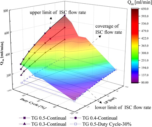
Adjusting the switching frequency is also an emerging route to enhance spray cooling performance, increasing spray efficiency, and reducing pumping power consumption [5,6]. This is important in some extreme conditions, such as aerospace applications, where the coolant flow rate is limited. It was used by NASA in the 1970s for active temperature control in the Flash Evaporator Subsystem to provide cooling for the Shuttle Orbiter vehicle during the ascent and re-entry phases [7,8]. Panão and Moreira [9,10] found that ISC provides coolant savings ranging from 10% to 90% compared with continuous spray cooling. Moreira and Panão [11] investigated the effect of switching frequency on heat transfer after multiple intermittent impacts from a hollow cone spray. An important feature of multiple- ISC is that the resulting liquid spray is pulsed and transient during the injection period due the pressure variations inside the liquid line.

In steady-state spray cooling, the heat flux is determined from the uniform temperature gradient between a series of thermocouples. During the highly transient process of ISC, the inverse heat conduction problem (IHCP) using internal temperature measurements is performed to obtain the time-varying thermal boundary conditions (e.g. heat flux at the surface). Although IHCP is used in other applications, the specified sequential function method (SFSM) and transform method are used in transient spray cooling. A Laplace transform can be used to determine the instantaneous heat flux from a temperature measurement at the surface [11–13]. The SFSM of Beck [14] is one of the most widely used algorithms for solving IHCPs. The function specification aspect is to represent the actual variation of $q(t)$ with a sequence of piecewise constant pulses of constant width. Regularization is performed using r future temperature measurements based on least squares regression to convert the ill-posed problem to a well-posed one. In ISC, the control strategy is always needed to be embed into the temperature measurement systems. For example, regarding the cooling of electronic devices, the control strategy (characterized by frequency and Duty cycle) should be modified instantly responding to the heat loads of the electronic devices. SFSM, a simple algorithm with fast response and open ports, is more applicable than other methods such as commercial software to be integrated into the control circuit of ISC.

Scholars have investigated the heat transfer performance of ISC. The application of SFSM in ISC has been addressed by the above studies. Almost all of them investigated the classical parameters related to SFSM algorithm for better prediction such as regularization, random noise and response time of thermocouple (time step). However, in ISC, the process parameter injection time or pulse period fundamentally represents the pulsed features of periodic steady state and the rate of variation of the transient heat flux. The relative effect between the injection time and time step would influence the criteria of degree of heat flux retrieval. In addition, evaluations of deterministic bias and standard deviation in the estimated heat flux need to be defined in ISC.

The objectives of the experiments are as follows: (1) introduce and determine the SFSM in a periodic steady state during ISC; (2) determine the effect of regularization, random noise, size of the time step in simulations, and pulse period on reproduction of the transient and averaged surface heat flux; (3) evaluate the deterministic bias and standard deviation in the estimated heat flux; (4) compare simulated and experimental results. The aim of this work is to address the simulated and experimental features of SFSM and to give a guidance of this algorithm for its application in ISC.

2. Experimental apparatus and procedure

The experimental system for spray cooling contains a water loop section, an electric heating section, a data acquisition section, and control section, as shown in Figure 2. The main parameters for the experimental devices are shown in Table 1. Deionized water was delivered with a gear pump (Micropump Co., Ltd) from a liquid tank. The deionized water was passed through a liquid filter (8 μm) and subsequently through a full-cone nozzle (Spray System TG SS). The nozzle was attached to a fast response solenoid (Parker Miniature Valves Series 9) valve to generate full cone sprays and provide intermittent spray control. A micro-positioning slide was bolted on the spray chamber to fix the nozzle at different heights and positions along the surface. The fluid was atomized and injected onto the heated surface in the spray chamber. The condensate and un-vaporized water were then cooled to a low temperature with a plate fin heat exchanger using a constant temperature water bath. The working fluid was then pumped back to the liquid tank in a closed loop.

Figure 2. Schematic of the experimental system.

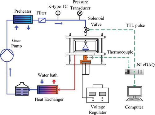
Table 1 Detailed information of experimental devices

Components	Manufacturer	Range
Nozzle	Spray System TG-0.4	1.5–10 bar
Data acquisition instrument	NI cDAQ 9212/9205	Maximum sample rate 95 Hz for temperature, 6.3 kHz for voltage
Geer Pump	Micro Pump PB23	For water:
		Max Diff-pressure: 8.7 bar
		Max flow rate:1000 ml/min
Solenoid valve	Parker Miniature Valves Series 9	Response time 6 ms, vac- 6.89 bar
Thermocouple	Omega GG-K-36	36 AWG, type-K
Pressure sensor	Danfoss AKS32	−1–12 bar
Cartridge heater	Omega CIR series	240 VAC, 500W

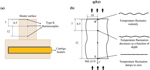
A heated copper block heater with 20 mm diameter was horizontally oriented in the experiments. It was electrically heated with four 500 W cartridge heaters, generating a maximum surface heat of 550 W/cm² (considering the heat loss). Heat loss from the sides and bottom were minimized by using nanometre porous materials and PTFE insulation. Three Type-K thermocouples, each 0.25 mm in diameter, were fixed into 0.5 mm-diameter holes in three layers along the depth of the block with the help of 316 steel wires (0.2 mm). The holes were sealed with thermal glue (Omega CC High Temperature Cement). The detailed mounting positions are shown in Figure 3.

Figure 3. One-dimensional inverse heat conduction problem (not scaled, unit: mm): (a) copper block; (b) calculating domain.

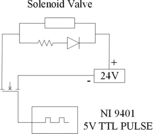
A data acquisition system (cDAQ, National Instruments) was used to gather data and control the system. The inlet pressure and temperature were measured with a pressure transducer and thermocouple that were situated upstream from the spray nozzle. Temperature measurements were gathered at 95 Hz using the NI 9212 high-speed thermocouple module. The pressure was measured at 1 kHz using the NI 9205 voltage input module. The pulsed spray control strategy is illustrated in Figure 4. The solenoid valve was driven with an NI 9401 TTL digital module, providing control over the frequency and pulse period. The actual injection time and non-injection time of nozzle are affected by two parameters: the response time of the solenoid valve; the flow inertia raised by the volume between the solenoid valve and the nozzle. The action of solenoid valve is delayed as the control signal is triggered from NI cDAQ system at not only the open action but also the shut action. Thus, the delay raised by response time of valve is actually a phase lag and has no effect on the actual injection time and non-injection time. Note that water in the volume is incompressible. After the spray system goes into fully period steady, the volume between the solenoid valve and the nozzle is full of water and the residual air inside is discharged. The pressure disturbance resulted from the open and shut action of valve would propagate to the nozzle orifice at a sufficiently quick speed (sound speed). Thus, the volume between the solenoid valve and the nozzle is believed to have less effect on the actual injection time and non-injection time. As a consequence, the analyses of pulsed features of ISC in the following sections are based on the injection time and non-injection time of the solenoid valve.

Figure 4. Illustration of the electronic control circuit for the solenoid valve.

The uncertainties in the measurements and from the experimental apparatus are given as follows. The accuracy of the pressure is ±0.39%. The response time of thermocouple is 10.5 ms. The thermocouples were calibrated using a Fluke 9144 metrology well (0.01°C) and a domestic ice point (0.1°C). Considering the uncertainty in measurements with the NI 9212 module, the uncertainty in the temperature measurements is approximately ±0.4°C. The absolute uncertainty of the distance between the surface thermocouple and the bottom thermocouple inside the heater block is ±0.25 mm. Another heat flux uncertainty originates from the surface temperature non-uniformity of spray cooling. It is well known that the heat transfer varies quite strongly in radial direction in spray cooling owing to the local distribution of the spray characteristics. In ISC, the instantaneous temperature history close to the surface is more suitable for obtaining accurate results for the surface heat flux [15]. However, the thermocouple of interest was greatly influenced by variations in the surface temperature, which can influence the accuracy of the surface heat flux calculation. To evaluate the effect of the surface temperature non-uniformity on the calculation of the surface heat flux, the heat fluxes of the one-dimensional Fourier's law and one-dimensional SFSM were compared. The heat flux of the Fourier's law was calculated from the temperature difference between different sensor layers which are far away from the surface and not influenced by the surface temperature uniformity. Please note that this type of heat flux uncertainty is a bias rather than a random noise. The maximal bias is −8.58%; the minus implies that the calculated SFSM heat flux is always underestimated owing to the surface temperature non-uniformity.

A 250 V AC voltage regulator was used to provide a heat load. Heat transfer from the bottom surface was considered to be in the steady periodic state when the deviation in the bottom temperature was less than 0.4°C.

3. Inverse heat conduction problem

A classic heat conduction problem is considered with the following restrictions and simplifications: (1) The thermal properties of copper block is temperature-independent; (2) Heat loss from the side is minimized and the corresponding boundary is considered heat isolated; (3) Heat is transferred from the bottom boundary at x = L and then is removed away from the surface by sprays at x = 0. Thus, the one dimensional heat conduction equation and boundary conditions are (1a) $\frac{{\mathrm{\partial }}^{2}T(x,t)}{\mathrm{\partial }{x}^2}=\frac{\rho c}{\lambda }\frac{\mathrm{\partial }T(x,t)}{\mathrm{\partial }t},$(1a) (1b) ${-\lambda \frac{\mathrm{\partial }T(x,t)}{\mathrm{\partial }x}|}_{x=0}=q(t),$(1b) (1c) $T(x,t){|}_{x=L}=T_L,$(1c) (1d) $T(x,t){|}_{t=0}=T_0.$(1d)

In steady-state spray cooling, the heat flux is determined from the uniform temperature gradient between a series of thermocouples, as shown in Figure 3(b). However, inasmuch as the time-varying surface heat flux $q(t)$ in Equation (1b) is difficult to measure directly in ISC, IHCP was used to calculate the heat flux from internal temperature measurements. The one dimensional classic future-time sequential-function-specification method of Beck [14] was used to determine the missing boundary in IHCP.

The function specification aspect is meant to represent the actual variation in $q(t)$ with a sequence of piecewise constant pulses of constant width, i.e. a stepwise heat input during each pulse. Under this assumption, the linear (inverse) problem can be expressed based on Duhamel's superposition integral. A discrete from of Duhamel's integral is defined as follows: (2) $T(x_i,t_M)=T_0+\sum _{n=1}^M{q}_n\mathrm{\Delta }{\phi }_{(M-n),}$(2) where $\mathrm{\Delta }{\phi }_{(M-n)}=\phi (x_i,t_{M-n+1})-\phi (x_i,t_{M-n})$ and $q_n$ are the values at the midpoint of a given time step representing the piecewise heat flux input between $t_{M-n+1}$ and $t_{M-n}$. $\phi$ is the unit impulse response and is the solution to Equation (1a–d) with a constant heat flux input of unit magnitude. $x_i$ is the temperature sensor location and the subscript i can be omitted for convenience because it was fixed in the present study. The estimated heat flux ${\hat{q}}_M$ at the current time $t_M$ can be easily obtained by rearranging Equation (2) [16].

Unfortunately, this is an ill-posed problem that requires regularization. The sequential estimation method of Beck [14] considers data from a number of r future times. This is a general case and was introduced in spray cooling by several researchers [15,17,18]. A short summary is described below.

First, Equation (2) is reformulated into a current temperature term and a previous information term: (3) $T_M=\mathrm{\Delta }{\phi }_0{q}_M+\sum _{n=1}^{M-1}{q}_n\mathrm{\Delta }{\phi }_{(M-n)}+T_0.$(3)

The temperature response at fixed location considering r future times can be expressed in the following form: (4) $\begin{array}{rl}{T}_{M+1}& =\mathrm{\Delta }{\phi }_1{q}_M+\mathrm{\Delta }{\phi }_0{q}_{M+1}+\sum _{n=1}^{M-1}{q}_n\mathrm{\Delta }{\phi }_{(M+1-n)}+T_0,\end{array}$(4) (5) $\begin{array}{rl}{T}_{M+r-1}& =\mathrm{\Delta }{\phi }_{r-1}{q}_M\cdots +\mathrm{\Delta }{\phi }_0{q}_{M+r-1}+\sum _{n=1}^{M-1}{q}_n\mathrm{\Delta }{\phi }_{(M+r-1-n)}+T_0.\end{array}$(5)

One can write this in matrix form as follows: (6) $\mathbf{T}=\mathbf{X}\mathbf{q}+{\hat{\mathbf{T}}}_i,$(6) where $\mathbf{X}$ is a sensitivity matrix, $\mathbf{q}=\{q_M,q_{M+1},\dots ,q_{M+r-1}\}$ and ${\hat{\mathbf{T}}}_i$ are the last two terms on the right in Equations (3)–(5) and the previous information term at $(M-1)\mathrm{\Delta }t$, respectively.

Under the assumption that $q_M=q_{M+1}=\cdots =q_{M+r-1}$, $\mathbf{X}$ can be rewritten as a diagonal matrix (7) $\left[\begin{array}{ccc}{\phi }_1& 0& \begin{array}{cc}0& 0\end{array}\\ 0& {\phi }_1& \begin{array}{cc}0& 0\end{array}\\ \begin{array}{c}⋮\\ 0\end{array}& \begin{array}{c}⋮\\ \cdots \end{array}& \begin{array}{cc}\begin{array}{c}\ddots \\ 0\end{array}& \begin{array}{c}0\\ {\phi }_1\end{array}\end{array}\end{array}\right].$(7)

The sum of the squared errors between the computed and measured values $S$ is (8) $S=\sum _{i=1}^r(y_{M+i-1}-T_{M+i-1}{)}^2=(\mathbf{Y}-\mathbf{T}{)}^T(\mathbf{Y}-\mathbf{T}).$(8)

Minimizing $S$ with respect to $\mathbf{q}$ yields (9) $\mathbf{q}=({\mathbf{X}}^{\mathrm{T}}\mathbf{X}{)}^{-1}{\mathbf{X}}^{\mathrm{T}}(\mathit{Y}-{\hat{\mathit{T}}}_i).$(9)

Solving Equations (6), (7), and (9) yields the estimated heat flux ${\hat{q}}_M$ (10) ${\hat{q}}_M=\frac{{\sum }_{i=1}^r{\phi }_i(y_{M+i-1}-{\hat{T}}_{M+i-1})}{{\sum }_{i=1}^r{\phi }_i^2},$(10) and the estimated surface temperature ${\hat{T}}_{M+i-1}$ (11) ${\hat{T}}_{M+i-1}=\sum _{j=1}^{M-1}{\hat{q}}_j\mathrm{\Delta }{\phi }_{M-j+i-1}.$(11)

The one-dimensional SFSM is a combination of Duhamel's integral deformation and the analytic solution to the forward problem. A solution (Equations (1a)–(d)) $\phi$ to a piecewise heat input must be calculated. This process differs in different IHCP systems.

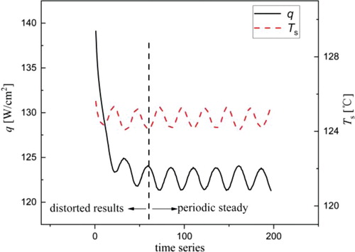
Equation (1a)–(d) contain three inhomogeneous boundary conditions. The boundary conditions in Equation (1a)–(d) with constant heat flux input at the bottom surface are similar to those used in other experiments [17]. It was reported that the surface temperature amplitude decreased with increasing depth in a steady periodic problem. In the present study, the temperature fluctuation in the bottom depth is less than 0.4°C, thus T_L can be considered constant. It is noteworthy that a temperature gradient appears in the block at t = 0, which results from the transient temperature field at t < 0 (can be considered 0⁻) and cannot be obtained using the thermocouple inserted in the block. The interest in our measurement is determining steady periodic heat conduction, thus the initial boundary (Equation (1b)) will not influence the final results as t increases continuously. Therefore, the temperature gradient in the domain at t = 0 is set to 0 in order to make the initial boundary (Equation (1b)) homogeneous. The temperature at x = L, t = 0 is considered the domain temperature. A series of distorted results would appear in the initial calculations using this assumption, as shown in Figure 5.

Figure 5. Calculated heat flux and temperature on the surface (using SFSM) where To = TL.

Thus, the direct problem using Equations (1a)–(d) in terms of $\theta (x,t)=T(x,t)-T_L$ is (12a) $\frac{{\mathrm{\partial }}^2\theta (x,t)}{\mathrm{\partial }{x}^2}=\frac{1}{\alpha }\frac{\mathrm{\partial }\theta (x,t)}{\mathrm{\partial }t}$(12a) $\begin{array}{}\text{(12b,c,d)}& -\lambda \frac{\mathrm{\partial }\theta (0,t)}{\mathrm{\partial }x}=q(t),\theta (\text{L},t)=0,\theta (x,0)=0.\end{array}$

To eliminate the inhomogeneity in Equation (12b), the temperature domain of the block is expressed using the transient and steady terms (13) $\theta (x,t)=\psi (x,t)+\varphi (x)$(13) such that $\varphi (x)$ includes the inhomogeneous boundary condition, the solution to which is (14) $\varphi (x)=\frac{q}{k}(L-x).$(14)

In terms of $\varphi (x)$, the transient problem $\psi (x,t)$ becomes (15) $\frac{\mathrm{\partial }\psi (x,t)}{\mathrm{\partial }t}=\alpha \frac{{\mathrm{\partial }}^2\psi (x,t)}{\mathrm{\partial }{x}^2},$(15) (16) $\psi (x,t)=-\varphi (x),-k\frac{\mathrm{\partial }\psi (0,t)}{\mathrm{\partial }x}=0,\psi (L,t)=0.$(16)

Using the separation constant, this classic characteristic-value problem gives the following solution [19]: (17) $\psi (x,t)=\sum _{n=0}^{\mathrm{\infty }}{a}_n{e}^{-a{\lambda }_n^{2}t}\cos ({\lambda }_{n}x),$(17) where $a_n$ is a Fourier coefficient. Hence, the dimensionless kernel function (18) $\phi (x^{+},t^{+})=\frac{\theta (x^{+},t^{+})-{\theta }_L}{qL}=1-x^{+}-2\sum _{n=1}^{\mathrm{\infty }}\frac{e^{-{({\lambda }_{n}L)}^2{t}^{+}\cos ({\lambda }_{n}L{x}^{+})}}{{({\lambda }_{n}L)}^2}.$(18)

MATLAB code for a one-dimensional IHCP with temperature history at one interior point was used to estimate the surface heat flux and surface temperature.

4. Numerical results

Regarding the IHCP, the data interpretation programme also performed uncertainty analysis of the heat flux and the heat transfer coefficient by sequentially perturbing the input values and accumulating individual uncertainty contributions [20,21]. This method is a statistical evaluation regarding noise in SFSM. An analysis of simulation results is presented in this section to provide insight into the accuracy of this method.

The key point is to decide whether the temperature history with the different experiment parameters can accurately reproduce the actual surface heat flux. Thus, the simulated surface heat flux to which the boundary condition is similar in the current experiment is described using Equation (19). DC = 50% and injection time$\mathrm{\Delta }{t}_{\text{inj}}$was $T/2$, and was equal to $\mathrm{\Delta }\overline{t_{\text{inj}}}$. (19) $q(t)\{\begin{array}{cc}300& T\times n\le t<T/2+T\times n\\ 3& T/2+T\times n\le t<T+T\times n\end{array}n=0,1,2\dots$(19)

The assumed heat flux profile $q(t)$ was performed using forward direct solution (Duhamel's integral) to obtain the interior temperature profile $T_n$ at depth x = 0.3 mm (dimensionless 1.58 × 10⁻²). In this process, the number of terms retained in the infinite series in the unit impulse response (or sensitivity coefficient) was sufficiently large (1000) and the time step size (1 ms) was sufficiently small. Thus, the interior temperature $T_n$ is considered to be an exact value without bias and noise.

Then, random noise was added by assuming that the measured temperature Y_n is equal to the exact temperature T_n plus some error ${\sigma }_n$ at each time t_n: (20) $Y_n=T_n+{\sigma }_n.$(20)

This temperature profile $Y_n$ was used as a boundary condition in SFSM in the numerical experiments to reproduce the heat flux. This temperature data was chosen with different regularization parameters (r = 1, 2, 3 … 8), different random noises ($\sigma$ = 0.4, 2, and 3°C), different time steps ($\text{d}t$ = 1, 5, and 10 ms) and different pulses ($\mathrm{\Delta }{t}_{\text{inj}}/\mathrm{\Delta }\overline{t_{\text{inj}}}$ = 13/13 and 165/165).

In the present experiment, most of the injection pulses were in the ∼10² millisecond range, which are larger than the time step of 10.5 ms. The shortest injection pulse was 13 ms with the same time step of 10.5 ms. The impulse would be omitted if the time step was larger than the impulse. Thus, pulses with periods of $T$ = 26 ms ($\mathrm{\Delta }{t}_{\text{inj}}/\mathrm{\Delta }\overline{t_{\text{inj}}}$ = 13/13) and 330 ms ($\mathrm{\Delta }{t}_{\text{inj}}/\mathrm{\Delta }\overline{t_{\text{inj}}}$ = 165/165) were examined. Parameters of the numerical experiments are shown in Table 2. There is a phase lag between the spray impact and the boundary heat flux in the above simulation process. The heat transfer performance on the surface and thermal inertia of cooper block between surface and thermocouple locations both result to this phase lag. However, zero phase lag is assumed in the present study since the focus herein is the surface heat transfer characteristics and this effect would be further investigated in future researches.

Table 2 Parameters of the numerical experiments.

	Regularization	Random noise [°C]	Time step [ms]	Injection duration [ms]	Period [ms]
Case 1	1,2,3,6	0.4	10	13	26
Case 2	2	0.4, 2	10	13	26
Case 3	2	0.4	1, 5, 10	13	26
Case 4	3, 6	0.4	1, 5, 10	165	330

4.1 Effect of regularization and random noise

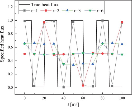
Regularization is used in SFSM to minimize random noise in highly transient temperature measurements. Figure 6 shows the estimated surface heat flux for r = 1, 2, 3, and 6 with 0.4°C of random noise. The maximum heat flux was set to unity. Regularization spreads the estimate of the pulses over more time steps and decreases their amplitude. This may indicate that surface heat transfer at high frequencies would fluctuate more heavily than we predict. Thus, we can consider the transient data is harmonically averaged due to deterministic bias to some degree. The deterministic bias for r = 2 is estimated to be 36.8% when $\mathrm{\Delta }{t}_{\text{inj}}\text{and}\mathrm{\Delta }\overline{t_{\text{inj}}}$ are both 13 ms, DC 50%, and 300 W/cm².

Figure 6. Comparison between the exact and estimated heat flux (dt = 10 ms, T = 26 ms) for different regularization parameters r.

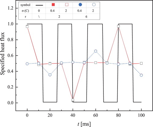
The temperature data used in SFSM was shown in the presence of different random noises (0.4 and 2°C) in Figure 7. No obvious difference can be found in the data with 0.4 and 2°C random noises. This is because the temperature measurement location is very near the surface and the effect of random noise is minimized.

Figure 7. Comparison between exact and estimated heat flux (dt=10 ms, T=26 ms) for different random noises σ.

4.2 Effect of time step and pulse period

Whether the temperature history with different measurement time steps can reproduce the actual surface heat flux must be verified. First, the time step does have an effect on how well the piecewise constant approximation to q(t) (i.e. the basic idea in Duhamel's integral) represents the actual function. The results for a 10 ms time step for r = 1 in Figure 6 represent the effect of time step on the piecewise constant approximation without considering regularization. Thus, deterministic bias due to the time step can be determined from the magnitude of the deviation from the exact heat flux at the time of each impulse. This was estimated to be 1.7% at 300 W/cm².

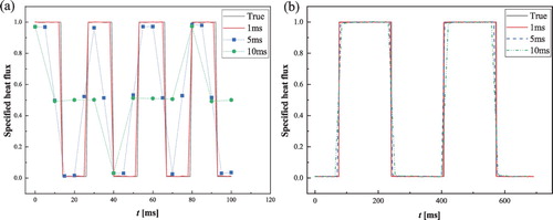
The temperature was measured with different time steps (1, 5, and 10 ms). The regularization parameter was r = 2 and the random noise was 0.4°C. One can see from Figure 8 that the relative time step length and injection duration are very important. When $\mathrm{\Delta }{t}_{\text{inj}}\text{ and }\mathrm{\Delta }\overline{t_{\text{inj}}}$ are both 13 ms, the results with 1 ms time step are more accurate than those with 5 and 10 ms. When $\mathrm{\Delta }{t}_{\text{inj}}\text{ or }\mathrm{\Delta }\overline{t_{\text{inj}}}$ is the same order as the current time step, the temperature measurement does not sufficiently reproduce the actual surface temperature and heat flux. Figure 8(b) shows a situation where $\mathrm{\Delta }{t}_{\text{inj}}$ and $\mathrm{\Delta }\overline{t_{\text{inj}}}$ are 165 ms, which is far larger than the time step. Slight differences can be seen for results with 1, 5, and 10 ms time steps when compared with the true value. Although increased time step results to increased bias, the reproduction degree of surface heat flux is still acceptable even for time step 10 ms. The curve with 10 ms time step has a smoother edge than those with 1 and 5 ms time steps. Bias exists primarily in the sharp edge of the curve, where the surface heat flux varies rapidly. Thus, the relative error in the calculated heat flux decreases with longer injection and smaller time step. This implies that, if injection time or pulse period is not considered, the evaluation based on time step only is insufficient.

Figure 8. Comparison between exact and estimated heat flux (r = 2 ms, $\sigma$ = 0.4°C) for different time steps $\text{d}t$: (a) T = 26 ms; (b) T = 330 ms.

Furthermore, despite the deterministic bias and random noise, one should note that the sum of the estimated heat flux components over all time steps in the above figures is equal to the simulated heat flux, i.e. conservation of energy is satisfied. This is important in spray cooling experiments. Because the heat removed from the bottom of the heat sink is always the interest during electronic thermal management, the averaged surface heat flux and temperature for each condition was used and the boiling curves were always used to evaluate heat transfer. In this aspect, black-box theory was used because the time-averaged value is equal to that using different r values and time steps, despite variations in heat transfer from the surface as a function of time. Thus, we can draw the conclusion that the deterministic bias induced by regularization and a coarse time step has no adverse effect on the boiling curve and predicted heat removal capacity.

4.3. Evaluation of deterministic bias and random noise

Conducting SFSM is a compromise between deterministic bias and random noise. The results from Section 4.1 are not significantly different from those in other studies and they show that random noise decreases as r increases, while the determined bias increases as r increases. Furthermore, the discussion in Section 4.2 shows that the bias and random noise also are influenced by the time step and pulse period (injection duration). Thus, another objective in the present study is to provide greater insight regarding the evaluation of bias and random noise.

The process for evaluating deterministic bias $B$ and standard deviation in the estimated ${\sigma }_q$ is described by Raynaud and Beck [22]. (21) $B={\left[\sum _{n=1}^m{(q_n-{\hat{q}}_n)}^2\right]}^{1/2}$(21) (22) ${\sigma }_q={\left[{\sigma }^2\sum _{n=1}^m{{\hat{q}}_n}^2\right]}^{1/2}$(22) where $\sigma$ is the random noise of temperature measurement, $q_n$ are the real values of heat flux and ${\hat{q}}_n$ are the calculated surface heat fluxes. Note that the definition from Raynaud and Beck is applicable to single pulses, therefore fixed points were used to calculate the surface heat flux. $B$ and ${\sigma }_q$ are independent of $m$ when $n$ is far from the impulse. However, there are periodic pulses in ISC and $B$, and ${\sigma }_q$ is time-dependent. Thus, we must decide whether points within the same time frame or points with the same counts of points are preferable. For example, if the same time frame is used, cases with $\text{d}t$ = 5 ms would contain 4 times as many points as cases with $\text{d}t$ = 20 ms. As a result, $B$ and ${\sigma }_q$ for $\text{d}t$ = 5 ms would be both higher than that with $\text{d}t$ = 20 ms, which violates the numerical results determined with SFSM in Sections 4.1 and 4.2. Thus, it is difficult to obtain a point-independent evaluation that provides a uniform benchmark for fair comparison. Tunnell et al. [15] used the same time frame to obtain the deterministic bias $B$ and standard deviation in the estimated ${\sigma }_q$. However, this adaption yields an incorrect representation of ${\sigma }_q$ in that ${\sigma }_q$ increases as $\text{d}t$ increases.

In the present study, points were calculated and the results were divided by the number of points. $B$ was determined from the square root of the sum of the squares of deviations between the estimated and true components: (23) $B=\frac{1}{N}{\left[\sum _{n=1}^m{(q_n-{\hat{q}}_n)}^2\right]}^{1/2}.$(23)

The sensitivity to measurement errors in the inverse algorithm is evaluated using (24) ${\sigma }_q=\frac{1}{N}{\left[{\sigma }^2\sum _{n=1}^m{{\hat{q}}_n}^2\right]}^{1/2},$(24) where N is the number of measured points and $\sigma$ is the random noise of temperature measurement. ${\hat{q}}_n$ are the calculated surface heat fluxes using a test temperature impulse as follows: (25) $Y^n=\{\begin{array}{c}\sigma n=s\\ 0n\ne s\end{array}.$(25) where $n$ has the same meaning as that in Equations (21)–(24). $s$ represents a certain value of n and it is randomly selected. The random noises are additive, uncorrelated, and have zero mean and constant variance ${\sigma }^2$. Therefore, the standard deviation of estimates ${\sigma }_q$ is the perturbation in the estimated surface heat flux due to random noise in the recorded temperature.

The following results in Figure 9 show this method sufficiently accounts for the effects of time step and injection duration. It shows a comparison of ${\sigma }_q$ versus $B$ for different regularization parameters r, random noises in the temperature $\sigma$, time steps $\text{d}t$, and periods of pulses $T$. One can see that ${\sigma }_q$ is inversely related to $B$ in all experiments. It also clearly shows the effect of the time step and periods of pulses on ${\sigma }_q$ and $B$. Increasing $\text{d}t$ and decreasing $T$ produces low resolution temperature measurements, yielding a high $B$ value. For example, regarding cases with $\text{d}t$ = 10 ms, $B$ with $T$ = 26 ms is higher than that with $T$ = 330 ms, yet ${\sigma }_q$ remains within the same range. Regarding the cases with $T$ = 26 ms, ${\sigma }_q$ and $B$ with $\text{d}t$ = 10 ms are both higher than the values found with $\text{d}t$ = 5 ms.

Figure 9. Comparison of standard deviation ${\sigma }_q$ versus bias B for different time steps $\text{d}t$ and pulse periods T.

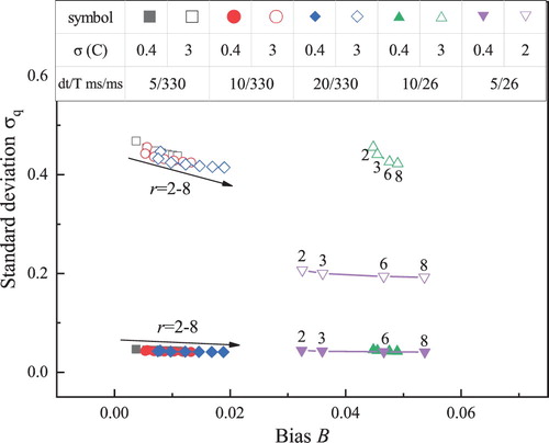
Meanwhile, the standard deviation of estimates ${\sigma }_q$ increases as $\text{d}t$ decreases but is independent of $T$. For example, regarding cases with $T$ = 330 ms, $B$ with $\text{d}t$ = 20 ms is higher than that with $\text{d}t$ = 5 ms, but ${\sigma }_q$ is inversely related to $\text{d}t$. This occurs because random noise in the temperature measurement is additive and the corresponding deviation ${\sigma }_q$ for the same time duration accumulates as $\text{d}t$ decreases and the number of calculated points increases. Further, the temperature measurement with high sampling rate would be strongly influenced by ambient noise in the experiments.

5. Experimental results

One can see from the Figure 10 that the magnitude of temperature and heat flux varies with the control voltage in ISC. Due to a superposition of an electromechanical delay, redundant fluid between the nozzle and the valve, and the thermal inertia raised by surface heat transfer between the spray impact and the heated copper block, there is a time delay between the control signal voltage and the temperature. In order to more conveniently display the parameter variations in the figure, the time delay was neglected so that the temperature changes as soon as the control voltage changes.

Figure 10. Typical fluctuations in control voltage, surface temperature, and heat flux at f = 2.5 Hz, DC = 80%, q = 122.8 W/cm² .

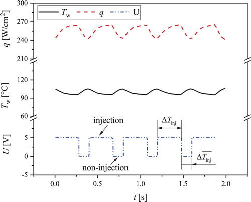
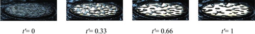
Figure 11 shows that the estimated curve shifts in time as the regularization parameter r increases. We must acknowledge that the transient curve is harmonically averaged to some degree due to deterministic bias. The actual curve may have a much sharper edge than we can predict. This is shown in Figures 6–8, where the commutative injection and non-injection behave like square waves. However, Figure 11 shows that the time variation in the experimental surface heat flux more likely behaves like a sine function, in contrast to the square wave for the simulated surface heat flux. This is because surface temperature history is altered due to dynamic heat transfer of residual liquid in non-injection period. Figure 12 shows the behaviour of residual coolant as a function of time during the non-injection time. Residual coolant persists for some time and evaporates, implying that heat transfer continues even when spray is not spurted on the surface. In addition, heat loss during non-injection period through the sides and the corresponding thermal inertia of the insulation maybe other possible reasons. In non-injection period, heat transfer through the liquid on the surface decreases and heat transfer through the sides can be significantly higher than that in injection period. In continuous sprays, the effect of heat loss is somewhat implicit in the results. However, in ISC, it would become more obvious. Finally, the response time of thermocouple would be another but not the major reason. The response time of 10.5 ms would reduce the resolution of the boundary of injection and non-injection. This makes the curve more round. However, the numerical study already reveals the effect of time step. The curves in numerical study varying time step from 1 to 10 ms all behave like a square wave. Thus, it is not likely that the response time of thermocouple would be the major reason.

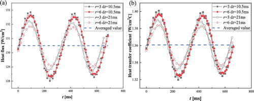
Figure 11. Calculated heat flux and heat transfer coefficient for r = 2, 3, 5, and 6, dt = 10.5 ms.

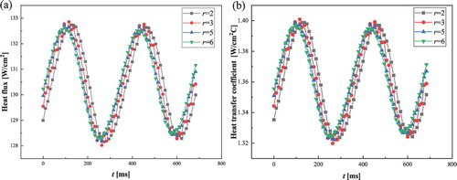
Figure 12. Transient behaviour of residual coolant on the heated surface in the non-injection duration ($\mathrm{\Delta }\overline{t_{\text{inj}}}$) at t′ = 0, t′ = 0.33, t′ = 0.66 and t′ = 1 $(t^{\mathrm{\prime }}=t/\mathrm{\Delta }\overline{t_{\text{inj}}})$.

In Figure 13, the averaged heat flux is the same as that determined with 10.5 ms time step, although the heat flux resolution for 20 ms time step is systematically dampened.

Figure 13. Calculated heat flux and heat transfer coefficient for dt = 10.5 and 21 ms with r = 3 and 6.

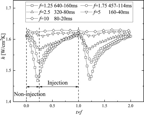
The SFSM result is the instantaneous surface temperature and heat flux. The transient heat transfer coefficient was estimated at each time step corresponding to the time steps during the temperature measurement. The corresponding heat transfer coefficient for DC = 80% as a function of time is shown in Figure 14. The temporal data for different pulse frequencies was rescaled to display two periods on the same axes. The heat transfer coefficient decreases sharply during the non-injection period and reaches a minimum value at the end of this period. The heat transfer coefficient increases rapidly after the injection period initializes. This shows that the heat transfer coefficient fluctuates more heavily at a lower frequency. The heat transfer coefficient fluctuates slightly for frequencies higher than 5 Hz while it fluctuates heavily as frequency declines below 2.5 Hz. Combined with the simulation results, one can conclude that the heat transfer coefficient for frequencies 5 and 10 Hz may fluctuate more heavily than we predict. This occurs because the corresponding non-injection durations are 20 and 40 ms and cannot include sufficient information regarding the temperature measurement with the current time step (10.5 ms). Regarding the cases for 2.5, 1.75, and 1.25 Hz, the IHCP estimates sufficiently reproduce the true heat transfer coefficient.

Figure 14. Heat transfer coefficient as a function of time with DC = 80%.

6. Conclusions

Simulations and experiments were performed to investigate the application of SFSM in ISC. The following are the key conclusions of this study:

1. SFSM is a compromise between deterministic bias and random noise. Regularization minimizes random noise in the temperature measurement but spreads the estimate for pulses over more time steps and decreases its amplitude.

2. The effect of time step and pulse period is very important in evaluating the deterministic bias and standard deviation in estimates. Increasing the time step and decreasing the pulse period decreases the resolution in the temperature measurement, yielding higher deterministic bias. For example, when the inject duration is the same order as the time step, information regarding the temperature measurement is insufficient and it is difficult to sufficiently reproduce the actual surface heat flux. However, increasing the time step would result in a smaller standard deviation in the estimates, while changing the period has no effect on this deviation.

3. The deterministic bias induced by regularization and coarse time step has no adverse effect on the boiling curves and predicted heat removal capacity.

In general, the control strategy of ISC is always based on the monitoring and control of surface temperature. However, the surface temperature is not consistent with the surface heat flux instantly owing to the thermal inertia of heat sink. This means that the surface temperature cannot represent the temperature information of the lower position of heat sink. Thus, a hypothesis maybe verified in future that the control strategy of ISC becomes a combination of both surface temperature and heat flux. In this point of view, it is important to better understand the transient features of surface heat transfer. In addition, a simple and useful method of IHCP such as SFSM is more applicable to be implanted into the control strategy.

Disclosure statement

No potential conflict of interest was reported by the authors.

Additional information

Funding

This work was supported by the National Natural Science Foundation of China under grant number 51876020, the Joint Fund of Equipment Development Department Pre-research Project and the Ministry of Education under grant number 6141A02022505.

References

- Cheng WL, Zhang WW, Chen H, et al. Spray cooling and flash evaporation cooling: the current development and application. Renew Sust Energ Rev. 2016;55:614–628. doi:10.1016/j.rser.2015.11.014.
- Somasundaram S, Tay AAO. Comparative study of intermittent spray cooling in single and two phase regimes. Int J Therm Sci. 2013;74(C):174–182. doi:10.1016/j.ijthermalsci.2013.06.008.
- Somasundaram S, Tay AAO. A study of intermittent liquid nitrogen sprays. Appl Therm Eng. 2014;69(1–2):199–207. doi:10.1016/j.applthermaleng.2013.11.066.
- Wang C, Song Y, Jiang P. Modelling of liquid nitrogen spray cooling in an electronic equipment cabin under low pressure. Appl Therm Eng. 2018;136:319–326. doi:10.1016/j.applthermaleng.2018.02.095.
- Liang G, Mudawar I. Review of spray cooling – Part 1: single-phase and nucleate boiling regimes, and critical heat flux. Int J Heat Mass Transf. 2017;115:1174–1205. doi:10.1016/j.ijheatmasstransfer.2017.06.029.
- Liang G, Mudawar I. Review of spray cooling – Part 2: high temperature boiling regimes and quenching applications. Int J Heat Mass Transf. 2017;115:1206–1222. doi:10.1016/j.ijheatmasstransfer.2017.06.022.
- Anderson M, Golliher E, Leimkuehler T, et al. Preliminary trade study of evaporative heat sinks. SAE Technical Paper 2006-01-2216, 2006. doi:10.4271/2006-01-2216.
- E.W. O’Connor, J.J. Zampiceni, N.F. Cerna and M.J. Fuller, “Orbiter Flash Evaporator: Flight Experience and Improvements”, SAE Technical Paper 972262, 1997. doi:10.4271/972262.
- Panão MRO, Correia AM, Moreira ALN. High-power electronics thermal management with intermittent multijet sprays. Appl Therm Eng. 2012;37(5):293–301. doi: 10.1016/j.applthermaleng.2011.11.031
- Panão MRO, Moreira ALN. Intermittent spray cooling: A new technology for controlling surface temperature. Int J Heat Fluid Flow. 2009;30(1):117–130. doi:10.1016/j.ijheatfluidflow.2008.10.005.
- Moreira ALN, Panão MRO. Heat transfer at multiple-intermittent impacts of a hollow cone spray. Int J Heat Mass Transf. 2006;49(21–22):4132–4151. doi:10.1016/j.ijheatmasstransfer.2006.04.004.
- Panão MRO, Moreira ALN. Thermo- and fluid dynamics characterization of spray cooling with pulsed sprays. Exp Therm Fluid Sci. 2005;30(2):79–96. doi:10.1016/j.expthermflusci.2005.03.020.
- Chen H-T, et al. Analytical solution of spray cooling characteristics on a hot surface using the Laplace transform. Inverse Probl Sci Eng. 2016;24(6):957–973. doi:10.1080/17415977.2015.1083990.
- Beck J, Woodbury K. Inverse engineering Handbook. Boca Raton (FL): CRC; 2002.
- Tunnell JW, Torres JH, Anvari B. Methodology for estimation of time-dependent surface heat flux due to Cryogen spray cooling. Ann Biomed Eng. 2002;30(1):19–33. doi: 10.1114/1.1432691
- Stolz JG. Numerical Solutions to an inverse problem of heat conduction for simple Shapes. J Heat Transfer. 1960;82(1):20–25. 10.1115/1.3679871.
- Somasundaram S, Tay AAO. A study of intermittent spray cooling process through application of a sequential function specification method. Inverse Probl Sci Eng. 2012;20(4):553–569. doi:10.1080/17415977.2011.639451.
- Zhou Z-F, Xu T-Y, Chen B. Algorithms for the estimation of transient surface heat flux during ultra-fast surface cooling. Int J Heat Mass Transf. 2016;100:1–10. doi:10.1016/j.ijheatmasstransfer.2016.04.058.
- Arpaci VS. Conduction heat transfer. Reading, MA: Addison-Wesley Publishing Co; 1966.
- Moffat RJ. Using uncertainty analysis in the Planning of an experiment. J Fluids Eng. 1985;107(2):173–178. doi:10.1115/1.3242452.
- Moffat RJ. Describing the uncertainties in experimental results. Exp Therm Fluid Sci. 1988;1(1):3–17. doi: 10.1016/0894-1777(88)90043-X
- Raynaud M, Beck JV. Methodology for comparison of inverse heat conduction methods. J Heat Transfer. 1988;110(1):30–37. doi:10.1115/1.3250468.