A reconstruction of object properties with significant uncertainties

ABSTRACT

An approach is developed to read and simulate experimental data using inverse problems. The idea is founded on a locally sequential refinement of the reconstruction. The regularization that occurs under a scheme of separate matching with observations is the basis for a numerical solution. The simultaneous identification of several unknowns using a set of mathematical models and functional representations of the desired quantities combines the simulation with inverse problem solutions. This unified approach is applied to the investigation of the enzyme kinetics. The object in question is simulated in the absence of information about the functional type of sought kinetic parameters, the noise structure and its level, and also details of observations. Nevertheless, the composition and volume of the samples under consideration prove to be sufficient not only for determining all of the kinetic parameters but also for clarifying the observation conditions. The obtained results demonstrate the effectiveness of the sequential regularized solutions to the inverse problems for the case of acting at once all the known features of ill-posed problems.

KEYWORDS:

• Simulation
• experimental data
• mathematical model
• parameter estimation
• identifiability
• regularization
• locally sequential refinement

Subject classification codes:

• 35K05
• 35R30
• 65J20
• 65R30
• 65N21

Nomenclature

a	=	parameters of a mathematical model
$\tilde{a}$	=	regularized parameters without full matching with errors
$\hat{a}$	=	regularized parameters minimizing residuals with samples
a(δ)	=	regularized parameters matching with consistency corridor
f	=	driving force
k-1, k1, k2	=	kinetic parameters
m	=	sample volume
p	=	number of parameters
t	=	time
u	=	direct problem solution (state function)
$\overline{u}$	=	actual state
u(δ)	=	sample
C	=	intermediate complex
C*	=	invariant state
E	=	enzyme
E0	=	initial value
I1,2	=	invariants
KM	=	Michaelis constant
$K_M^{(0)}$	=	regularized estimate using the Michaelis–Menten function
${\hat{K}}_M$	=	regularized estimate using the inverse problem solution
$L_a$	=	mathematical operator depended on parameters $a$
N	=	number of approximation nodes
P	=	penalty function
P	=	product
S	=	substrate
S0	=	initial value
S*	=	invariant state
S(δ)	=	sample
$\overline{S}$	=	actual state
Tm	=	final time of observations
Tobs	=	observation grid
${\tilde{T}}_{obs}$	=	regularized grid of observations without full matching with errors
${\hat{T}}_{obs}$	=	regularized grid of observations minimizing residuals with samples
$T_{obs}^{(\delta )}$	=	regularized grid matching with consistency corridor
V	=	production rate
V(δ)	=	sample
$\overline{V}$	=	actual state
$\hat{V}$	=	regularized state
Vmax	=	maximum reaction rate
$V_{max}^{(0)}$	=	regularized estimate using the Michaelis–Menten function
${\hat{V}}_{max}$	=	regularized estimate using the inverse problem solution
	=	functional space
$\mathfrak{M}$	=	measure of solution complexity
δ	=	upper bound of noise
$\epsilon$	=	noise
γ	=	residuals of the observation matching equations
ρ	=	residuals with observations
τ	=	grid of sought quantity approximaxion
ν	=	absolute estimation error
χ	=	nodes of approximaxion
Π	=	penalty coefficient
X	=	vector of parametrization
Ω	=	stabilizer

1. Introduction

The investigations of new objects and processes are characterized, as a rule, by the absence of essential information regarding their phenomenological properties. In such cases, the study can be accomplished using an inverse problem in which the unknown object properties are included in the composition of the desired solution. The uniqueness of the sought quantities’ reconstruction is established by obtaining additional observations and conditions toward a direct problem’s solution. The additional data should preserve the one-to-one correspondence between the sought quantities and samples.

Traditionally, an inverse problem formulation is considered to be an extension of a parental direct problem [1–8]. However, methodologically, inverse problems can be used in more contexts than as a solution to a single problem. In [9], the application of inverse problems in the form of a specific sequence was proposed to solve all of them with the same initial data. Accordingly, the experimental data can be simulated in the framework of not just a single inverse problem but also within a specific set of such formulations. Here, the simulation reflects the adequacy of the model in question as a discrepancy with an observation set and clearly shows the directions of further modelling, which should improve an obtained discrepancy with samples. The simulation with solutions to a series of inverse problems facilitates the object’s investigation in the absence of a significant amount of initial data on phenomenological properties, and when there exist definitional uncertainties.

In general, the requirement of solving a series of inverse problems extends the solution domain. The extension can occur at all levels of the simulation. As known, these levels include 1) a problem formulation, where a solution character is defined; 2) a functional representation, wherein an approximation of the desired functions is performed; and, of course, 3) calculations, wherein the final discrete form of the problem in question can be ill-conditioned or weakly sensitive to variations of unknowns.

As introduced by [10], the primary requirement for solutions to ill-posed problems is the restriction of feasible states to boundaries that are consistent with errors in the initial data. This principle should also be used to formulate the sequence of regularized solutions to inverse problems. Correspondingly, the critical condition of the correct identification is the sequence formation that narrows down the choice of arbitrary elements at each simulation level. The approach for specifying such a sequence depends on the initial information, and different ideas can be suggested.

An inductive sequence of solutions to inverse problems can restrict numerical oscillations during the changes of the object model and during the transitions of its approximation. This idea was proposed in [9]. The required sequence is performed as a transition from the simple model of an object to a more complex one while at the same time drawing on the previous identification. The initial choice of a simple model with its gradual complication together with the regularization of the solution at the calculation level facilitates the necessary restrictions of a solution domain.

A decomposition sequence of solutions to inverse problems also turns out to be an effective means of limiting feasible object states if there are far more uncertainties in the investigation of the object on the whole than in studying any part of it. The formulation of the inverse problems in the case of splitting a complicated object into components and studying only one of them was considered in [11].

The present paper considers a case when an extension of a solution domain is associated with introducing a significant number of, for example, discretization nodes. This extension is typical for complicated functions. Their reconstruction within a single inverse problem solution requires a large number of measurements, which are often not possible to obtain. In this case, the sequential solutions to a series of inverse problems can also be useful. As in the above matters with induction and decomposition approaches, the necessary restrictions are implemented by the gradual transition from a simple form of an approximation to more complicated species. At the calculation level, the control of the variations of the sought solution is realized by the minimization of stabilizing functionals [10]. In the end, the identification – in accordance with the principle ‘from simple to extended’, including the mandatory regularization – allows for a significant reduction of numerical instability when the mathematical formulation has uncertainties.

Thus, the same set of experimental data is proposed, associating with a set of inverse problems, functional representations, and numerical stabilization procedures. The developed approach will reveal the object’s properties, for which other known methods require postulating and introducing an essential volume of initial data. For all three simulation levels, which were mentioned earlier, the feasible states of an object will be restricted, and solutions to inverse problems will be matched with the noise of initial data. As a result, the structure, properties, and features of the object under study are identified in detail despite the existence of substantial uncertainties regarding initial information and sought quantities.

The idea of serial solutions to similar problems is widespread in both numerical mathematics and the theory of complex systems. Among the numerical methods, the relaxation method is commonly known [12,13]. Also, multigrid methods [14] first compute an approximation on a coarser grid – usually the double spacing – and use that as a solution with interpolated values for the other grid points as the initial assignment. In mathematical programming [15], a difficult problem is approximated by a simpler problem whose ‘relaxed’ solution provides information about the solution to the original problem. The proposed solutions to a series of inverse problems and a locally sequential refinement of a functional representation – together, they express a sequence of regularized solutions – are similar to the relaxation idea. Here, a simpler problem is an identification of a separate component of the sought quantity.

In [16,17], the sequential regularization method has been proposed. The technique is a functional iteration procedure for solving direct problems with isolated singularities. It has been introduced to improve a stiff numerical scheme of solutions to direct problems. Below the sequence of regularized solutions is used for other purposes. The first objective is solutions to a series of inverse problems to reconstruct unknowns in the framework of expansive uncertainties. The second objective is the extension of sought quantity approximation. Because of this, the object modification is controlled at each simulation level.

In the context of optimization theory, the most closely related field is that of robust optimization and robust control [18,19]. Commonly known that the optimization often has a high sensitivity to perturbations in the problem parameters. Robust optimization develops the idea that a solution should be constructed, satisfying any implementation of the uncertainty in a given set. The locally sequential refinement of the reconstruction initially involves filtration of uncertainties. The best choice of a regularized element is based on a stabilizer minimizing together with a sample matching when standard optimization methods are applied. Especially important for a satisfactory reconstruction is that the condition not to exceed the interval of concentration should be met. If the latter condition is introduced into robust optimization procedures, then the approaches will be close together. It may be noted that the local sequential refinement essentially proposed below offers a robust optimization for a solution to inverse problems without the postulation of the uncertainty kind.

Along with the regularization of inverse problems, machine learning is being widely developed to identify complicated objects [20–22]. However, in the framework of machine learning, an object is not considered as a whole, and it is assumed that although identifying the complete object may not be possible, determining specific patterns or regularities can be useful. In contrast, the simulation with inverse problems is based on a sequence of transitions from a simpler to a more general object description, where patterns are not postulated and can be determined by solutions to inverse problems.

Other approaches can also be used to identify complex functions. Among them are neural networks [23,24], nonparametric regression and classification techniques [25–28]. The main difference of these methods with the locally sequential refinement is the adaptive regularization of the sought quantity reconstruction. The approaches mentioned above do not have this feature. However, namely, this feature makes possible the transition from a strongly smoothed solution to its detailing.

Certainly, the essential requirement of the correct solution to the inverse problem is a performance of conditions ensuring the uniqueness of reconstruction and the identifiability of desired parameters. Justifying unambiguity requires considerable theoretical efforts [1,2,5,29,30]. In this direction, the practical results can be achieved by excluding the manifestation of an invariant family in a solution to a direct problem [31]. This idea is implemented below to prove the identifiability of parameters of enzyme kinetics.

The case study will be chosen to demonstrate how a traditional simulation methodology can be improved because, in terms of machine learning, the patterns of the object are obtained on the whole. Though the object in question is widely used in biosciences, at present, inverse problems regarding this object are not solved because there are essential numerical difficulties for the identification without the regularization [32].

The paper is organized as follows. In Section 2, an abstract inverse problem is formulated to use a large class of mathematical models and to reconstruct different representations of unknowns in a series, taking into account the required changes in the simulation of the object. Section 3 describes how it should regularize the numerical solutions without a known regularization parameter, while at the same time, taking into account all features of simulation and observations. In Section 4, the locally sequential refinement of a functional representation is proposed to restrict local violations of a monotone behaviour occurring in desired quantities during the reconstruction. In Section 5, the mathematical model and features of the object under study are formulated. Section 6 is devoted to the identifiability of the kinetic parameters. The conditions of the simultaneous reconstruction of all the kinetic parameters of the model in question are defined. Section 7 formulates the solutions to the series of inverse problems and facilitates the identification of an extended number of unknowns within significant uncertainties in the source data. Section 8 describes the alternative solution to control the proposed approach. Section 9 demonstrates the approach application for processing the experimental data of enzyme kinetics. Section 10 summarizes the obtained results.

2. An abstract inverse problem

Consider a general formulation of an inverse problem, which can cover a range of simulation questions. A broad class of mathematical models, a set of desired quantities, and various representations of unknowns are involved in order to perform their modification, which is necessary during simulation procedures.

Let the model of the object in question be given in a domain space (1) $L_{a}u=f,$(1) where u is a direct problem solution that denotes an observable state function, f is a known external excitation (an abstract ‘driving force’), a=$\{a_k{\}}_{k=\overline{1,p}}$, p ≥ 1 is the unknown object’s properties, and La denotes a continuous operator that acted in a Banach space and whose ranges of values are also a Banach space.

The existence of a unique element u for the given a and f is supposed everywhere below. It is also assumed that, generally, the operator $L_a$ does not need to have a continuous inverse operator $L_a^{-1}$. Besides, it is assumed that the domain of Eq. (1) is not a compactum at . These conditions will play a key role, when quantities a = $\{a_k{\}}_{k=\overline{1,p}}$ are estimated with general assumptions about their functional properties and when a broad class of mathematical models is involved [10]. The condition of the parameter’s unidentifiable limits the number of unknown quantities. This condition for the superposition of the linear operators was obtained in [31].

No restrictions are put on the form of the operator L_a. Any mathematical model can be used with both the lumped and the distributed parameters. Both analytical and numerical methods can be applied in solving the direct problem (1). The drawback in the latter case is the usual stumbling block for numerical analysis, that is, a loss of the generality power of the obtained results.

It is required that one seek the function u and its parameters a = $\{a_k{\}}_{k=\overline{1,p}}$, p ≥ 1 with a minimal estimation error $\nu =\overline{a}-a$ when a sample $\{u_i^{(\delta )}{\}}_{i=\overline{1,m}}$ is given to have a prototype $\overline{u}$ on the discrete set $\mathrm{\Xi }=\{{\xi }_i{\}}_{i=\overline{1,m}}$ (or the measurement points) from a known observation space, such as (2) $\begin{array}{rl}{u}_i^{(\delta )}& =\overline{u}{|}_{{\xi }_i}+\epsilon {|}_{{\xi }_i},i=\overline{1,m},\end{array}$(2) (3) $\begin{array}{rl}\Vert \epsilon {|}_{{\xi }_i}\Vert & \le {\delta }_i,i=\overline{1,m},\end{array}$(3) where the approximately known element $u^{(\delta )}$ deviates from the prototype $\overline{u}$ on each statistically independent m group by a known amount, (4) $\Vert u_i^{(\delta )}-\overline{u}{|}_{{\xi }_i}\Vert \le {\delta }_i,i=\overline{1,m}.$(4)

Here $\epsilon$ is any function, including random ones, with the known and limited measure (3) on each element of the observation set Ξ; $\{{\delta }_i\}{|}_{i=\overline{1,m}}$ denote the noise internals of concentration; and m is the number of statistically independent elements of Ξ.

The prototype $\overline{u}$ is the solution to Eq. (1) with an actual (‘true’) quantity $\overline{a}$, $\overline{u}=L_{\overline{a}}^{-1}f$. The number m characterizes the sample size. For the present study, this number is not significant and has a minimum value satisfying the identifiability conditions [31]. Such a sample is defined everywhere below as a sample of limited size.

Note that some features of the formulation (1) – (4) are essential for the developed approach.

The observation model (2), (3) conveys a broad class of noise sources and facilitates the study of many valuable cases of measurements. One of them is a sample with a bound volume, while the other is the nonzero level of the noise. It is also possible to account for the simulation and systematic measurement errors. Any hypothesis regarding the distribution of noise does not need to be introduced, and the expected value and covariance matrices are not specified. Only the measure (3) is considered to be known.

Eq. (2) expresses the direct measurements. If necessary, any other representation can also be contemplated, for instance, when the observations are a function of the state u (see Section 7). The norm of condition (4) is the standard estimator of the noise level. It is possible to use, for example, the rms norm or the absolute norm, which can be derived in any experiment. The selection determines the accuracy of the estimation. The choice of the norm of condition (4) was considered in [33–35].

Condition (4), which is called the observation matching equations below, is one of the basic premises for determining the unknowns. It requires providing the proximity between the observed $u^{(\delta )}$ and the model-calculated $u{|}_a$ states by the noise level separately carried out for each given sample. If the desired quantities are the vector-functions (p > 1), then condition (4) requires the observations to be set as statistically independent groups.

3. Regularization under separate matching with observations

The critical roles of the sequential solutions to a series of inverse problems are the restriction of numerical variations in sought quantities and matching a solution with a measurement noise level. The latter should be less than the threshold level, which disturbs the parameter’s identifiability (for more details, see [36]). At the calculation level, the methods that meet these requirements are called the regularized methods. The regularization principles were introduced and justified in [10].

The choice of the regularization approach is defined by the simulation features of the problem in question. For further discussion, the following premises are essential.

1. The proposed simulation implies different types of inverse problems, including the coefficient inverse problem, the boundary inverse problem, and others. The regularization should be easily adapted for all.

2. The regularization should be sufficient for any model of an object.

3. Several model parameters or functions may be unknown, so the sought quantities are the vector-functions with which multiple samples of a state function should be associated.

4. The reconciliation with the observations should be separately carried out for each given sample, which contrasts the generalized matching condition (5) $\Vert u^{(\delta )}-u\Vert \le \delta ,\delta =\underset{1\le i\le m}{max}|{\delta }_i|.$(5)

5. traditionally used in the regularization theory [10]. Here, it is necessary to take into account that the condition (5) leads to a deliberately biased solution for a nonzero interval of concentration, δ ≠ 0, because of the primarily multipoint set $\{{\xi }_i{\}}_{i=\overline{1,m}}$ will be transformed into a single point scheme, and the system of m conditions (4) is reduced to the sole condition (5) (for more details, see [33]).

6. The values of $\{{\delta }_i{\}}_{i=\overline{1,m}}$ are neither negligible nor improvable quantities, and the reconciliation should be fulfilled when the asymptotic tendency of the noise to zero is not considered as such (for more details see [36]).

7. Features of a solution to a direct problem are considered to be known, and the regularization should be able to include this information into the reconstruction procedures.

Among the known approaches for solutions to ill-posed problems, such as the Tikhonov regularization [10], Morozov discrepancy principle [37], Ivanov quasi-solution [38], and iterative regularization [39,40], all the requirements from a) – f) are met by the regularization scheme [33]. This scheme is methodologically based on theory [10] and, in particular, addresses the model identification and parameter estimation from the standpoint of the abstract inverse problem (1) – (4). This regularization is determined as the following formulation.

The reconstruction of unknown parameters a = $\{a_k{\}}_{k=\overline{1,p}}$ of Eq. (1), using a noisy sample $u^{(\delta )}$ with the known measure (3) and providing the necessary restriction and consistency, is reduced to the variational problem: (6) $a^{(\delta )}=Arg\underset{a\in A_L}{\inf }\mathrm{\Omega }[a],A_L=\{a:L_{a}u=f,\Vert u_i^{(\delta )}-{u|}_{{\xi }_i}\Vert \le {\delta }_i,i=\overline{1,m}\},$(6) where Ω[a] denotes a continuous and nonnegative functional, the domain of which involves the sought parameters a.

The scheme (6) requires determining element a^(δ), which minimizes the preset functional Ω when the direct problem solution u is matched with the noise level separately for each element of the observation set $\{u_i^{(\delta )}{\}}_{i=\overline{1,m}}$. This functional Ω is defined as a stabilizer because its minimization ensures the restriction of the solution domain. Also, the functional Ω is the complexity measure of the desired solution. Its inclusion in the minimization criterion facilitates choosing the best element a^(δ) among all possible estimates in the sense of attaining a minimum of the complexity measure of the desired solution [10]. Below, it will be shown how the stabilizer ensures the solution’s stability (see subsection 9.2).

As for the theoretical substantiation of the scheme (6), note that the inverse problem is reduced to the nonlinear programming problem. The substantiation of both the existence and the uniqueness of the solution to the abstract problem (6) has known difficulties. The uniqueness of the parameters’ reconstruction of the abstract operator L_a can be challenging to prove. At the same time, if the specific object is considered, then it is possible to obtain the particular conditions of solvability for the problem in question (see Section 6).

Concerning the regularization scheme (6), there are some noteworthy features.

The main difference between the scheme (6) and other known regularization approaches is the requirement to be partially fitted with the noise level for each element of the set $\{u_i^{(\delta )}{\}}_{i=\overline{1,m}}$. The scheme (6) has not the regularization parameter [10] because the stabilizer Ω is directly minimized. Note as well that in [33], the non-optimality of the traditional Tikhonov’s scheme with a regularization parameter was demonstrated when the desired solution was a vector function. The scheme with the regularization parameter cannot match the desired solution with the noise level separately for each element of the observation set. However, the Tikhonov’s scheme facilitates the dominant technique for investigating general mathematical properties of ill-posed problems. The scheme (6) is especially useful when the noise level has the nonzero and improvable value, and several unknown quantities are simultaneously estimated [9,11,33–35].

This scheme (6) can be applied to solve a wide array of inverse problems. Its application does not depend on the kind of mathematical model used, which can be either a multidimensional or a nonlinear equation with both lumped and distributed parameters. Any required degree of regularization is realized according to the chosen approximation of the unknowns [33–35]. Any quantitative and qualitative preliminary information of both the unknowns and the state function can be introduced into the reconstruction procedures. For example, it can be information about monotonous behaviour as a direct problem solution and as reconstructed functions. A variety of parameters of the object in question are supposed to be simultaneously estimated if the one-to-one correspondence between the direct problem solution and sought quantities is satisfied. It will be demonstrated below that the scheme (6) facilitates attracting the conditions of the unique solution to the inverse problem.

The application of the scheme (6) in practice is better suited for standard mathematical methods. A penalty function for a finite-dimensional basis $\mathrm{X}=\{{\chi }_k{\}}_{k=\overline{1,N}}$ is introduced as follows: (7) $\mathrm{P}(\mathrm{X})=\mathrm{\Omega }[\mathrm{X}]+\sum _{i=1}^m{\mathrm{\Pi }}_{i}max\{0,{\gamma }_i(\mathrm{X})\},$(7) where ${\gamma }_i=\Vert u_i^{(\delta )}-u{|}_{{\xi }_i}\Vert -{\delta }_i$ are the residuals of the observation matching equations, Πi denotes penalty coefficients, and N denotes the number of discretization nodes. The piecewise linear basis $\mathrm{X}$ is used in Section 9. The penalty function (7) reduces the variational problem (6) to the unconstrained programming problem for the parameterization vector $\mathrm{X}$. Known algorithms and software can be used to determine its solution. For the simulation below, the algorithm of the coordinate descent will be used.

4. A locally sequential refinement of a reconstruction

The numerical oscillations can occur both in general and local kinds. For the first case, the solution at each point of its region can differ significantly from the solution at the neighbouring point. This case, which is known as high-frequency oscillations, is being intensively studied. Several regularized techniques are being proposed to restrict the oscillations in general [2–8,10,16,37–41]. For the second case, a local disturbance of a monotonous behaviour of desired quantities occurs. These kinds of the low-frequency oscillations are typical for a large volume of a discretization set (see Section 9). At present, insufficient attention is paid to the regularization of the low-frequency oscillations.

Having proposed the restriction of the desired solutions in general by the scheme (6), we will implement the relaxation rules for solutions to ill-posed problems. The reconstruction should be based on the elementary step, which consists of varying only one element of the set of unknowns, and the number of variable elements being chosen in a specific cyclic order. The restriction technique described below is the essential addition to the stabilizer’s implementation because local disturbances of a monotonous behaviour will be bounded for the cases, where the stabilizer cannot exclude the appearance of spikes.

It is well-known that for ill-posed problems, applying a general type of an initial approximant is incorrect because its domain will contain an unordered set of elements. Very often, a priori information on the functional type of sought quantities is absent. However, the specific features of the solution to the direct problem – the position of extremum, the inflection and intersection points, the monotonicity, and similar others – are known. This essential information can be implemented in the locally sequential refinement of the functional representations of the unknowns. Their steps are described below.

4.1. First step: the simpler approximation

Generally, the reconstruction should be started with the simpler approximation of the sought quantity, for example, with constant values. By this simplification, the discrepancy between the observation set $u^{(\delta )}$ and the direct solution $u{|}_a$ will significantly exceed the measurement noise level. However, this solution may already express the critical functional properties of the observed object state and – importantly – can show the areas in which the discrepancy with the observations is the highest. A difference between features of a solution and observed state functions reflects the zones of the unsatisfactory consistency with the experimental data.

For example, the displacement of a calculated position of some function feature from its observed place shows the presence of a simulation error. Also, the monotonous behaviour of both the desired quantities and direct problem solutions can be controlled effectively. In the case of interrelated processes, the control can be accomplished by checking positions, which express the inception of growth or drop of each interrelated part of a process (for more details, see subsection 9.2).

The question regarding the convergence of the approach described above is solved by controlling the level of the changes in the functions being identified. Any known norm, such as the root mean squares or the absolute deviation, can be used measuring changes of a new solution relative to its previous version. The stabilizing functional is the convenient target, which can be applied for such control.

4.2. Second step: the local refinement of a part of the desired quantity

Further reconstruction should be implemented as a local refinement. The specification of sought elements is performed only within a separate local zone when other elements of the vector of unknowns remain unchanged. The latter is taken from the previous solution.

The local refinement is performed for the parts with a weak discrepancy or a consistency violation between the functional properties of a direct problem solution and observations. For example, the previously introduced constants can be dissected into the parts according to the established zones of the poor discrepancies. After this, the transition from a piecewise constant function to a piecewise linear approximation can be performed together with the sequential solutions to the inverse problems for each step of the transformations. Any other approximants can be applied.

The criterion of satisfactory detailing is the determination of a smaller discrepancy for given samples, as well as the improvement of a certain degree of the sought solution complexity, which, for example, can be a stabilizer.

The refinement bounds are determined by both the complexity of the function being identified and the sample size. In particular, a variant that adds only one new node in the selected zone can be considered.

4.3. Third step: the refinement expansion

Each extension of the approximation requires the regularization. It should be implemented starting from the local zone and finishing on the whole range of observations. The necessary stabilization during the step-by-step reconstruction is described in Section 3.

Additionally, if it is required, any other ideas of restrictions, for example, the descriptive regularization [41] can be applied. The scheme (6) can combine the stabilizer with the application of all of them. In such a combination, the stabilizer restricts the solution throughout the domain space, and the additional local regularization realizes the solution smoothing when the weak sensitivity generates the disturbance of the solution’s monotonicity in a local zone. These restrictions together provide the regularization of both the high- and low-frequency numerical oscillations.

As a result, the reconstruction during the sequential change from the refined zone to the whole area of the observation can match the current size of the parameterization set with the sample volume. The initially determined solution, which has the highest restrictions on the sought functions, is transformed from its neighbourhood and checked for its variations. The locally sequential refinement – and, at the same time, the regularized reconstruction from the neighborhood of the previously determined solution – should be performed until the required consistency with the given observations is reached, and the solution complexity will be minimized.

4.4. Fourth step: the refinement expansion

The proposed sequence of the transitions differs from the approximation extension, which is usually applied in theory. As a standard, the solution is sought in the entire function domain after the extension. Here — and this is imperative — the reconstruction is implemented for only a portion of a finite-dimensional basis of approximation, as defined by the worst residual. The next step of the extension is accomplished by using another weak discrepancy or by using the differences between the observed and calculated features of the solution to the direct problem. The scheme is analogous to the relaxation methods but differs from them by its implementation of a portion on a finite-dimensional basis.

The required minimum volume of the experimental data should reflect the basic functional properties of observed states, such as smoothness, non-negativity, monotonicity, convexity, and others. They are supposed to be known. These characteristics facilitate controlling the reconciliation with the observations at a qualitative level. It is desirable to observe these characteristics experimentally because the choice of the refinement zone is based on them.

At the quantitative level, determining the volume of the necessary information is the subject of a separate problem of the experimental design. The design method that takes into account the noise action and provides the necessary regularization is proposed in [42].

The level of the changes in the identified functions has allowed controlling the convergence of the proposed approach. Any known norm, such as the root mean squares or the absolute deviation, can be used measuring changes of a new solution relative to its previous version. The stabilizer is a convenient target, which can be applied to such control.

The justification of the proposed method of a complex function reconstruction is based on the following conditions: i) the minimization of residuals chosen sequentially from the worst value to the general minimum magnitude, ii) the construction of the sought solution approximation according to the principle from the simple to the complex one, iii) the transition to the next simulation step from the vicinity of the previous solution, iv) the regularization of both the high- and low-frequency numerical oscillations, v) the control over the reduction of the selected complexity criterion of the solution, and vi) the obligatory fulfillment of the requirement of compliance with the specific features of observed states such as the maximum position, the inflection and intersection points, the regions of the solution monotonicity, and similar features.

Thus, the locally sequential refinement is the solution to a series of similar problems implemented the procedures for the isolation of problem singularities on each simulation level by the sequential regularized transactions from a partial to a general kind of a sought quantity approximation.

5. The object in question

Consider time-dependent kinetics of irreversible biomedical reactions. One of the most investigated processes in bioscience is a substrate transformation into a product under the catalytic influence of an enzyme [43]. This kinetic is based on the so-called Henri-Michaelis–Menten scheme and is applied to a variety of spheres, including alveolar filtration of dust, the richness of species pools, filtering alcohol from the blood, and many others.

The choice of this object is made because, in bioscience, there are many investigations, where the commonly known Michaelis–Menten function gives essential simulation errors. At present, the change of the fitting function is accomplished as ‘a black box’ approximation without directly accounting any object features. In contrast, the developed simulation with inverse problems can directly account for any known, or observed object properties and substantiate the required modification of the fitting function. Especially emphasize that, namely, the correct reconstruction of sought parameters can reflect the actual functional kind of the observed discrete set.

It is necessary to keep in mind that there is no a priori information about the functional character of the parameters of enzyme kinetics. In general, they should be seen as time-dependent functions. However, at present, the mathematical simulation of enzyme kinetics has been made in the framework of the constant kinetic parameters. This simplification reflects the overall picture of the object’s dynamics. Nevertheless, from the viewpoint of mathematical modelling, this leads to an unsatisfactory discrepancy between the experimental data and state function calculated by the mathematical model. In particular, many experiments show a significant difference between the observed and model-calculated states obtained with the constant parameters. Processing of the experimental data in Section 9 confirms the existence of similar modelling errors. Thus, the determination of the nature of the parameters of enzyme kinetics is a critical point of the object simulation. The latter is the purpose of the present study.

5.1. The direct problem

According to the Henri-Michaelis–Menten scheme, the enzyme E reacts with the substrate S to form an intermediate complex C, which then, under the action of the enzyme, forms a product P and releases the enzyme. These objects are schematically represented as the reaction: (8) $E+S\underset{\underset{k_{-1}}{⟵}}{\overset{\stackrel{k_1}{⟶}}{}}C\stackrel{k_2}{⟶}E+P,$(8) where k_-1 and k₁ are the microscopic rate parameters, and k₂ is the catalytic parameter.

The mathematical model of the object (8) can be obtained by applying the law of mass action [44]. As a result, the time evaluation of the object is entirely determined by a pair of coupled equations: (9) $\begin{array}{rl}\frac{dS}{dt}& =-k_1(E_0-C)S+k_{-1}C,t>0,\\ \frac{dC}{dt}& =k_1(E_0-C)S-(k_{-1}+k_2)C,t>0\end{array}$(9) together with an uncoupled equation (10) $\frac{dP}{dt}=k_{2}C,t>0$(10) having the initial conditions (11) $S{|}_{t=0}=S_0,C{|}_{t=0}=0,P{|}_{t=0}=0.$(11)

The direct problem (9) – (11) is known as the Briggs–Haldane equations of enzyme kinetics [45].

Additionally, basic Eqs. (9) – (11) obey two conservation laws: (12) $\begin{array}{rl}E(t)+C(t)& =E_0,\\ S(t)+C(t)+P(t)& =S_0.\end{array}$(12) These equations determine the necessary and sufficient set of the state functions S(t), C(t), E(t), P(t), which fully characterize the object in question. If the function P(t) is sought from Eq. (10), then the accuracy of the numerical solution to the direct problem is determined from Eq. (12).

Note that everywhere below, the dimensions of the kinetic parameters $k_{-1},k_1,k_2$and the state functions S(t), C(t), E(t), P(t) are omitted in order not to overload the paper with information that is not used. Formally, this most straightforward procedure of the dimensionless is permissible because each parameter can be sorted with its identity dimension value, and the original equations will be transformed into a dimensionless form. Because of this, the focus is on the mathematical aspects of the reconstruction.

5.2. The features of the direct problem

The known solutions to the Briggs–Haldane equations described in [46–48] have expressed the features of the enzyme kinetics. The typical behaviour of the state functions S(t), C(t), E(t), P(t) for the constant parameters $k_{-1},k_1,k_2>0$ are shown in Figure 1.

Figure 1. Typical behaviour of the solutions to the direct problem (9) – (11).

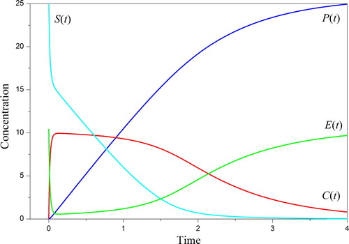
Note that there are three areas with the crucial significance, namely, i) the narrow interval at the initial stage, ii) the middle part with the slow varied function C(t), and iii) the final phase of the process. Below, it will be demonstrated that the observations in these areas ensure the best reconstruction. Consequently, the exclusion of observations in these areas excludes obtaining the necessary information about the peculiarities of solving the direct problem. This notation does not close the question of the optimal design and determining the best observations should be separately considered.

Traditionally, investigations of enzyme kinetics are based on the property of the direct problem (9) – (11), which is known as the quasi-steady-state approximation [49] and is described, in detail, in the literature [50–53]. The state is considered to be appropriate in cases, where the enzyme concentration is small compared with the substrate concentration. This ration of the components occurs when the enzyme is first mixed with a large amount of a substrate. There exists an initial period during which the complex concentration accumulates. The reaction quickly achieves a steady state in which complex C remains approximately constant over time. Then, from Eqs. (9) – (12), it follows (for example, see [53]) that the production rate $V\equiv dP/dt$ depends on the concentration of a substrate as the function (13) $V=\frac{V_{max}}{K_M+S},$(13) where $V_{max}$ is the maximal reaction rate that can be attained when the substrate concentration is so large that the entire enzyme exists in form C, and $K_M$denotes the substrate concentration at the half-maximal rate. The hyperbola (13) is known as the Michaelis–Menten function.

In the characterization of an enzyme, it is essential to know the optimal concentration of substrates. This concentration relates to the values $V_{max}$ and $K_M$. Their estimations are easily realized from the observation fitting by the hyperbola (13) and using the nonlinear regression technique. The estimations come from the approximation by the Michaelis–Menten function have severe limitations.

The magnitude V_max is the asymptote of the hyperbole (13) for S → ∞. Therefore, the function (13) does not reflect the properties of the direct problem solution, $S{|}_{t\ge 0}\le S_0$ and $V{|}_{S=S_0}=0$. The function (13) is obtained for the quasi-steady state so measurements on the entire observation space $T_{obs}\in [0,\mathrm{\infty })$ are not considered. It is also necessary to take into account that the function (13) proposes the only usage of the constant parameters, $k_{-1},k_1,k_2=const$. Because of the hyperbolic nature of the function (13), the estimation of the parameters $V_{\text{max}}\text{ and }{K}_{\text{M}}$ is always biased relative to their actual values.

5.3. The inverse problem

The peculiars mentioned above are avoided by moving to the inverse problem. Their solutions will approximate the object in question more accurately than the hyperbole (13). The inverse problem is formulated as follows.

The existence, uniqueness and stability of the solutions to the Briggs–Haldane equations are supposed to be satisfied. For the object with the state function u = {S(t), C(t), P(t), E(t)}, two samples, (14) $\begin{array}{rl}{S}_i^{(\delta )}& =\overline{S}(t_i)+{\epsilon }_1(t_i),\underset{1\le i\le m}{max}|{\epsilon }_1(t_i)|\le {\delta }_1,i=\overline{1,m},\\ & V_i^{(\delta )}=\overline{V}(t_i)+{\epsilon }_2(t_i),\underset{1\le i\le m}{max}|{\epsilon }_2(t_i)|\le {\delta }_2,i=\overline{1,m},\end{array}$(14) are known. The measurements are performed at the same observation time $T_{obs}=\{t_i{\}}_{i=\overline{1,m}}$. The parameters {$k_{-1},k_1,k_2>0$} should be estimated using the samples $S^{(\delta )}$ and $V^{(\delta )}$. Their prototypes $\overline{S}$ and $\overline{V}\equiv k_2\overline{C}$ are satisfied by Eqs. (9) – (11).

The identification of the kinetic parameters makes it possible to read the observations (14) and reveal all the features of the object (8) by reconstructing the functions S(t), C(t), E(t), P(t). The functional type $k_{-1},k_1,k_2$ will express the character of the microscopic rate, catalytic process, and production rate. By this, the simulation with inverse problems will give essential information regarding the enzyme kinetics and will answer the question about the adequate representation of its parameters.

5.4. The reconstruction features

To say anything in advance about the functional kind and character of kinetic parameters is impossible. They can be either constant quantities or variable functions. For Eqs. (9) – (11), it turns out to be characteristic that, even for small discrepancies between the functions S and V and their observations $S^{(\delta )}$ and $V^{(\delta )}$, there are significant variations of the desired quantities $k_{-1},k_1,k_2>0$, which are met by small changes of the direct problem solutions {S, V} (see subsection 9.2). This case requires a regularization, which will be accomplished by the scheme (6).

For the sake of definiteness in the framework of the present paper, the inverse problem is defined as the traditional formulation, where composition and the volume of initial data are enough to identify the model’s parameters in the framework of a single formulation. For estimating enzyme parameters, the traditional formulation was considered in [24]. In the framework of its formulation, the features of the object were not determined.

At the same time, the experimental schemes, which are usually used for studying enzyme reactions, have several characteristic traits. They transform the traditional formulation of the inverse problem into the simulation by the solutions to a series of inverse problems (see Section 7). It is necessary to take into account the following features.

The nature of the information that usually comes from the enzyme experiments [54] requires additional identification of the initial values $S_0,E_0>0$. The extension of a number of the unknowns raises the question of invariant subset existence and necessitates determining the conditions that segregate the desired parameters from the invariant subset. The identifiability of the kinetic parameters is studied in Section 6.

The observation model (14) needs the values δ_1,2, which express the within-sample scatter and determine the boundaries of the consistency corridor of the state functions with their observations. For the cases of experimental data considered below, the essential feature is the absence of any information about the noise. Nevertheless, the scheme (6) can reveal the approximate valuation of the boundaries of the consistency corridor. Their values are determined by a simple reception, which is described in Section 7.

Along with the above, it is necessary to take into account that descriptions of enzyme experiments, as a rule, do not contain information about the observation time T_obs. The absence is because of the existing practice of researches on enzyme reactions. If two samples {$S^{(\delta )}$,$V^{(\delta )}$} are obtained, then the sample $V^{(\delta )}$ is approximated by the function (13), and its parameters $V_{max}$ and $K_M$ are estimated. Because of this, no observation times T_obs are required. A similar approach is extensively applied in practice [46]. Despite the widespread use of this approach, its application provides an estimate of only a limited number of process parameters and requires special experimental conditions for the implementation of a quasi-steady-state.

Thus, in contrast to the estimation of the function (13) parameters $V_{max}$ and $K_M$ there is a statement regarding the inverse problem, which allows for the features of the enzyme kinetics to be identified. The inverse problem in question differs from the traditional formulation because of the lack of data on the initial conditions, the noise level, and the observation times. Nevertheless, the conjugacy of the functions S(t) and V(t) makes it possible to expand the composition of the unknowns and to reconstruct the observation time, $T_{obs}=\{t_i{\}}_{i=\overline{1,m}}$ together with the parameters a = {k_-1, k₁, k₂, S₀, E₀}. The upper bounds of the noise δ_1,2 are estimated using the residuals of the observation matching equations.

Note that if kinetic models are more complex than (9) – (11) and there are possibly additional intermediate steps as well as no explicit relation between the functions V and S, then it will be necessary to obtain complete information on the observation conditions and also to require an experiment, where the identifiability conditions must be satisfied. The conditions for Eqs. (9) – (11) are determined below.

6. The identifiability of the kinetic parameters

The extension of a number of the unknowns necessitates substantiating the uniqueness of the simultaneous reconstruction of all the parameters a = {k_-1, k₁, k₂, E₀, S₀}. If the class of the invariant solutions to the direct problem are determined and the conditions of their existence are revealed, then the criteria of the parameter identifiability are defined ex contario. Such approach effectiveness has been shown in [31] to justify the identifiability even for the existence of invariant properties.

6.1. Propositions

Let us study the invariant properties of the direct problem (9) – (11) relatively its parameters. Suppose that for the solution {S*(t), C*(t), P*(t), E*(t)}∈ * there corresponds a subset of two different vectors, $a^{\mathrm{\prime }}=\{k_{-1}^{\mathrm{\prime }},k_1^{\mathrm{\prime }},k_2^{\mathrm{\prime }},E_0^{\mathrm{\prime }},S_0^{\mathrm{\prime }}\}$ and $a^{\mathrm{\prime }\mathrm{\prime }}=\{k_{-1}^{\mathrm{\prime }\mathrm{\prime }},k_1^{\mathrm{\prime }\mathrm{\prime }},k_2^{\mathrm{\prime }\mathrm{\prime }},E_0^{\mathrm{\prime }\mathrm{\prime }},S_0^{\mathrm{\prime }\mathrm{\prime }}\}$, where $a^{\mathrm{\prime }}\ne a^{\mathrm{\prime }\mathrm{\prime }}$∈A*={a: $L_{a^{\mathrm{\prime }}}^{-1}f\equiv L_{a^{\mathrm{\prime }\mathrm{\prime }}}^{-1}f$ }. Any continuous functions k_{- 1}(t), k₁(t), k₂(t) and constant E₀, S₀ = const > 0 are considered.

The transformation $a^{\mathrm{\prime }}\to a^{\mathrm{\prime }\mathrm{\prime }}$ and the invariant family A* should be determined, which does not change the direct problem solution. Grounded in the conditions of the existence of family A*, the criteria for the identifiability of all the kinetic parameters will be gained.

6.2. Invariants of the Briggs–Haldane equations

Substituting the parameters $a^{\mathrm{\prime }}$ and $a^{\mathrm{\prime }\mathrm{\prime }}$ in Eqs. (9) – (11) and subtracting these equations from each other, the conditions $k_2^{\mathrm{\prime }}=k_2^{\mathrm{\prime }\mathrm{\prime }}$, $S_0^{\mathrm{\prime }}=S_0^{\mathrm{\prime }\mathrm{\prime }}$ are obtained. This result means that the solution u = {S, C, P, E} to the problem (9) – (11) is not invariant relative to the parameters k₂ and S₀. However, the functions {S, C} are invariant with respect to the parameters k_-1, k₁ and E₀. For the latter case, the intermediate complex C depends on the substrate S as the function (15) $C^{\ast }=I_1\frac{S^{\ast }}{S^{\ast }+I_2}$(15) where $I_1=\frac{k_1^{\mathrm{\prime }\mathrm{\prime }}{E}_0^{\mathrm{\prime }\mathrm{\prime }}-k_1^{\mathrm{\prime }}{E}_0^{\mathrm{\prime }}}{k_1^{\mathrm{\prime }\mathrm{\prime }}-k_1^{\mathrm{\prime }}}$ and (16) $I_2=\frac{k_{-1}^{\mathrm{\prime }\mathrm{\prime }}-k_{-1}^{\mathrm{\prime }}}{k_1^{\mathrm{\prime }\mathrm{\prime }}-k_1^{\mathrm{\prime }}}$(16) are the invariants of Eqs. (9) – (11). The initial value C|_t=0 imposes the condition (17) $I_1{{|}_t}_{=0}=0.$(17)

The existence of the invariants I₁ and I₂ indicates that any functions {S, C}, satisfied by Eq. (9), can be associated with the transformation (18) $k_{-1}^{\mathrm{\prime }\mathrm{\prime }}=k_{-1}^{\mathrm{\prime }}+I_2{k}_1^{\mathrm{\prime }}\frac{E_0^{\mathrm{\prime }\mathrm{\prime }}-E_0^{\mathrm{\prime }}}{I_1-E_0^{\mathrm{\prime }\mathrm{\prime }}}$(18) (19) $k_1^{\mathrm{\prime }\mathrm{\prime }}=k_1^{\mathrm{\prime }}\frac{I_1-E_0^{\mathrm{\prime }}}{I_1-E_0^{\mathrm{\prime }\mathrm{\prime }}},$(19) which preserves the solutions {S, C} over the domain of Eq. (9), and *≡ . Thus, for the general case, the reconstruction of the vector-function a = {k_-1, k₁, k₂, S₀, E₀} is impossible.

6.3. Identifiability criteria for the states with invariant properties

If the sought parameters are positively defined, k_-1, k₁, k₂, E₀, S₀ > 0, then the additional conditions are obtained for invariants: (20) $\begin{array}{rl}& 0\le I_1<{E_0}^{\mathrm{\prime }}<{E_0}^{\mathrm{\prime }\mathrm{\prime }},\end{array}$(20) (21) $\begin{array}{rl}& I_2{{|}_t}_{=0}<0.\end{array}$(21)

The transformation (19), taking into account (20), yields $k_{-1}^{\mathrm{\prime }\mathrm{\prime }}{|}_{t=0}<k_{-1}^{\mathrm{\prime }}{|}_{t=0}$. Further, from (16), (17) and (19), it follows that $I_2{|}_{t=0}=-\frac{{k_{-1}^{\mathrm{\prime }\mathrm{\prime }}|}_{t=0}-{k_{-1}^{\mathrm{\prime }}|}_{t=0}}{{k_1^{\mathrm{\prime }}|}_{t=0}}\frac{E_0^{\mathrm{\prime }\mathrm{\prime }}}{E_0^{\mathrm{\prime }\mathrm{\prime }}-E_0^{\mathrm{\prime }}}.$

Then, taking into account (20) and (21), the condition $k_{-1}^{\mathrm{\prime }\mathrm{\prime }}{|}_{t=0}>k_{-1}^{\mathrm{\prime }}{|}_{t=0}$ is determined.

Therefore, in the vicinity of the initial stage of the enzyme process, t ∼ 0, the transformations (18) and (19) for the positively defined parameters will lead to an increase of any transformed coefficient $k_{-1}^{\mathrm{\prime }\mathrm{\prime }}$ regarding its parental value $k_{-1}^{\mathrm{\prime }}$ and a decrease of any $k_1^{\mathrm{\prime }\mathrm{\prime }}$ relative to $k_1^{\mathrm{\prime }}$. This condition expresses the criterion for choosing the desired elements from the invariant family (18) and (19) because, at the initial stage of the enzyme process, the parent parameter k_-1 always has the minimum value while the parent parameter k₁ always has the maximum value among all the elements of the invariant family.

In order to fully express the conditions of the invariant transformations (18), (19), it is necessary to determine the initial values $I_2{|}_{t=0}$ and $k_{-1}^{\mathrm{\prime }\mathrm{\prime }}{|}_{t=0}$. To do this, from (15), it is determined ${\frac{dC}{dt}|}_{t=0}={\frac{d{I}_1}{dt}|}_{t=0}\frac{S_0}{S_0+{I_2|}_{t=0}}.$

On the other hand, from Eq. (9), it follows that ${\frac{dC}{dt}|}_{t=0}=k_1{|}_{t=0}{E}_0{S}_0.$

Finally (22) $I_2{|}_{t=0}={\frac{d{I}_1}{dt}|}_{t=0}\frac{1}{E{}_0^{\mathrm{\prime }}{k{}_1^{\mathrm{\prime }}|}_{t=0}}-S_0,$(22) and $k_{-1}^{\mathrm{\prime }\mathrm{\prime }}{|}_{t=0}=k_{-1}^{\mathrm{\prime }}{|}_{t=0}-\frac{E_0^{\mathrm{\prime }\mathrm{\prime }}-E_0^{\mathrm{\prime }}}{E_0^{\mathrm{\prime }\mathrm{\prime }}{E}_0^{\mathrm{\prime }}}\left({\frac{d{I}_1}{dt}|}_{t=0}-S_0{E}_0^{\mathrm{\prime }}{k_1^{\mathrm{\prime }}|}_{t=0}\right).$

In the end, for any functions S and C satisfied by Eq. (9), it is possible to specify the new parameters (18), (19), which will not change the values of a pair {S, C} in the whole domain of Eq. (9). The invariant I₁ is any function that satisfies conditions (17) and (20), and the invariant I₂ is specified as the function I₂ = S(I₁/C – 1), which should have the initial condition (22). The invariant family does not exist for the constant parameters, {k_-1, k₁, k₂, E₀, S₀ = const}, because of I₁ ≡ 0 for any t.

As proved, the parameters S₀ and k₂ do not belong to the invariant subset. Further, if the sought parameters are positively defined, k_-1, k₁, k₂, E₀, S₀ > 0, then the parental values k_-1|_t = 0 and E₀ always have the minimum, and k₁|_t = 0 the maximum magnitudes among any other ones from the invariant subset. These conditions express the criteria of the unique estimation of the vector-function a = {k_-1, k₁, k₂, E₀, S₀} as the parental element of the invariant family (18), (19). The relevant criteria should be involved in the reconstruction procedure.

6.4. Invariant property illustrations

Let us demonstrate the above-revealed character of the invariant transformation. Consider the parental parameters (23) $\begin{array}{rl}{k}_{-1}& =10/[1+50exp(-2t)],k_1=10/(2t^2-5t+4)+1,\\ k_2& =3/[10/(2t^2-6t+4)+1]+1,S_0=100,E_0=20.\end{array}$(23)

Figures 2 and 3 show the various I_1,2, for which the transformations (18), (19) save the functions S and C for $E_0^{\mathrm{\prime }\mathrm{\prime }}=30$. The transformed parameters are depicted in Figures 4 and 5. They express the features of the invariant transformation regarding the minimum and maximum values of the parental parameters k_-1 and k₁.

Figure 2. Invariant I₁ of the problem (9) – (11) with the parameters (23): 1 – $I_1^{(1)}=\frac{10t}{2t^2-5t+4}$; 2 – $I_1^{(2)}=-0.1t(t-20)$; 3 – $I_1^{(3)}=\frac{15t}{t+50\exp (-t)}$; 4 – $I_1^{(4)}=\frac{2.95t}{1+0.01\exp (0.05t^2)}$.

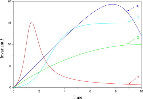
Figure 3. Invariant I₂ = S(I₁/C – 1) of the problem (9) – (11) with the parameters (23) and various I₁: 1 – $I_1^{(1)}=\frac{10t}{2t^2-5t+4}$; 2 – $I_1^{(2)}=-0.1t(t-20)$; 3 – $I_1^{(3)}=\frac{15t}{t+50\exp (-t)}$; 4 – $I_1^{(4)}=\frac{2.95t}{1+0.01\exp (0.05t^2)}$.

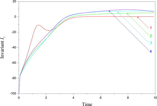
Figure 4. The parameters k_-1 from the invariant subset (18): 1 – the parent function from (23), 2 – transformed by$I_2^{(1)}$, 3 – transformed by $I_2^{(2)}$, 4 – transformed by $I_2^{(3)}$, 5 – transformed by $I_2^{(4)}$.

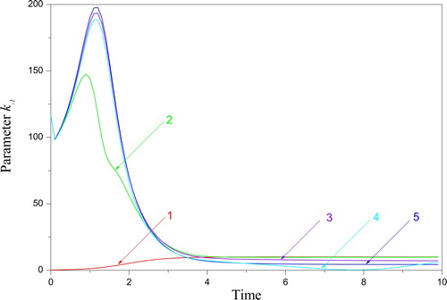
Figure 5. The parameters k₁ from the invariant subset (19): 1 – the parent function from (23), 2 – transformed by $I_1^{(1)}$, 3 – transformed by $I_1^{(2)}$, 4 – transformed by $I_1^{(3)}$, 5 – transformed by $I_1^{(4)}$.

Thus, there are conditions of the unique estimation of the parameters a = {k_-1, k₁, k₂, E₀, S₀} despite the existence of the invariant properties of the problem (9) – (11).

7. The inductive sequence of inverse problems

Now, the sequence of the subproblems identifying the extended complex of unknowns $\{a,T_{obs}\}$ will be introduced. For the case discussed below, the sequence should implement the inductive principle ‘from a partial to a general’, because the volume of initial information is insufficient. In the framework of the formulations, the transitions will be performed by controlling the solution’s complexity measure.

7.1. First subproblem: entirely consistent with the sample

The reconstruction of the observation time $T_{obs}=\{t_i{\}}_{i=\overline{1,m}}$ should be started from the case when the state function S(t) is entirely consistent with the first sample, $S(t_i){|}_a=S_i^{(\delta )},i=\overline{1,m}$, and the discrepancy with the second sample $V^{(\delta )}$ is minimized regarding the desired parameters a = {k_-1, k₁, k₂, S₀, E₀}. The regularized solution $\tilde{a}$ and ${\tilde{T}}_{obs}=\{{\tilde{t}}_i{\}}_{i=\overline{1,m}}$ is determined as the following subproblem: (24) $\begin{array}{rl}\tilde{a}& =Arg\underset{a>0}{\text{inf}}\{{\mathrm{\Pi }}_1\mathrm{\Omega }[a]+{\mathrm{\Pi }}_2\sum _{i=1}^m[V({\tilde{t}}_i){|}_a-V_i^{(\delta )}{]}^2\},\\ & S({\tilde{t}}_i){|}_{\tilde{a}}-S_i^{(\delta )}=0,i=\overline{1,m},\end{array}$(24) where the state functions S and V are determined as the solution to the direct problem (9) – (11).

The solution to subproblem (24) is central to the running simulation because it defines the observation grid ${\tilde{T}}_{obs}$ that is consistent with the experimental data as much as possible. The observation grid, in turn, entirely defines the further identification of the kinetic parameters. However, in subproblem (24), the measurement errors of the sample $S^{(\delta )}$ are not taken into account and ${\tilde{T}}_{obs}$ are sought without any restrictions to the variations of the state functions.

Here, the determination of the element ${\tilde{T}}_{obs}$ is considered as the initial approximation for the next subproblem. Its necessary restriction and reconciliation with the noise level will be fulfilled during the next steps in the framework of the second and third subproblems. The choice of the stabilizer Ω[a] is determined by the functional properties of desired quantities and is described in Section 9. The spherical norm of matching conditions in (24) is introduced to facilitate the convexity of the target function.

7.2. Second subproblem: the upper bound of the reconstruction error

Obtained the initial guess of the observation grid ${\tilde{T}}_{obs}=\{{\tilde{t}}_i{\}}_{i=\overline{1,m}}$, the further estimation requires accounting the interval of concentration of the sample $S^{(\delta )}$. Because of the heterogeneity of the unknowns a and T_obs, this subproblem is divided into two parts. First, the vector $\hat{a}$ is sought for the given grid $T_{obs}=\{t_i{\}}_{i=\overline{1,m}}$. Accordingly, the constraints of the parameters k_-1, k₁, k₂, S₀, E₀ are provided, and the discrepancy for each sample is minimized. Second, the grid ${\hat{T}}_{obs}$ is reconstructed using the previous estimate $\hat{a}$. The initial values $\{a,T_{obs}\}$ are taken from the solution to subproblem (24). The important advantage over the previous subproblem is the account of the difference between the model-calculated function and its observations, $S(t_i)\ne S_i^{(\delta )},i=\overline{1,m}$. The difference has significance for nonzero measurement errors.

According to the scheme (6), the regularized reconstruction $\{\hat{a},{\hat{T}}_{obs}\}$ is reduced by the penalty function to the following sequentially solved extremal problems: (25) $\begin{array}{rl}\hat{a}& =Arg\underset{a>0}{inf}\left\{{\mathrm{\Pi }}_1\mathrm{\Omega }[a]+{\mathrm{\Pi }}_2\sum _{i=1}^m{[V{({\hat{t}}_i)|}_a-V_i^{(\delta )}]}^2+{\mathrm{\Pi }}_3\sum _{i=1}^m{[S{({\hat{t}}_i)|}_a-S_i^{(\delta )}]}^2\right\},\\ {\hat{T}}_{obs}& =Arg\underset{T_{obs}>0}{inf}\left\{{\mathrm{\Pi }}_4\mathrm{\Omega }[T_{obs}]+{\mathrm{\Pi }}_2\sum _{i=1}^m{[V{(t_i)|}_{\hat{a}}-V_i^{(\delta )}]}^2+{\mathrm{\Pi }}_3\sum _{i=1}^m{[S{({\hat{t}}_i)|}_a-S_i^{(\delta )}]}^2\right\}.\end{array}$(25) Here, the requirements for limiting the growth of the sought quantities $a\text{and }{T}_{obs}$ are accomplished because their stabilizers Ω[a] and Ω[T_obs] are minimized. The choice of the stabilizers is determined by the functional properties of desired quantities and is described in Section 9. The spherical norm of matching conditions in (25) is introduced to facilitate the convexity of the target function.

The solution to subproblem (25) gives the values of the worst residuals for each sample: ${\rho }_S=\underset{1\le i\le m}{\text{max}}|S{({\hat{t}}_i)|}_{\hat{a}}-S_i^{(\delta )}|,{\rho }_V=\underset{1\le i\le m}{\text{max}}|V{({\hat{t}}_i)|}_{\hat{a}}-V_i^{(\delta )}|.$

The obtained values of the residuals ${\rho }_{S,V}$ include the uncertainties of the simulation and the measurements. If the noise levels ${\delta }_{1,2}$ are known, then it is possible separating the obtained residuals ${\rho }_{S,V}$ on the simulation and the measurement errors and estimating the level of the simulation error ζ under the condition ζ = max{(ρ_S - δ₁), (ρ_V - δ₂)}. In the case of the unknown noise level ${\delta }_{1,2}$, the values ${\hat{\delta }}_{1,2}$ are introduced, for which all the residuals between the samples and the regularized solution to the next subproblem do not exceed ${\hat{\delta }}_{1,2}$. Such a technique is an effective way to estimate the boundaries of the consistency corridor ${\hat{\delta }}_{1,2}$.

It should be noted that the above-described technique does not make the lack of information about measurement errors an insignificant factor. The knowledge of the noise level ${\delta }_i$ remains an essential part of the inverse problem formulation.

7.3. Third subproblem: matching into the framework of the consistency corridor

Now, the regularization of the desired elements $\{a,T_{obs}\}$ is being implemented for those values ${\hat{\delta }}_1\le {\rho }_S,{\hat{\delta }}_2\le {\rho }_V,$ starting from which the reconciliation with each of the samples (14) is satisfied and the stabilizers for both the observation grid T_obs and vector a = {k_-1, k₁, k₂, S₀, E₀} are minimized. Mainly, this subproblem should impose the maximum functional limitations of the desired elements. The corresponding regularized solution $\{a^{(\delta )},T_{obs}^{(\delta )}\}$, consistent with the errors, is determined from the following extremal subproblems: (26) $a^{(\delta )}=Arg\underset{a>0}{inf}\mathrm{\Omega }[a],\underset{1\le i\le m}{\text{max}}|S{(t_i)|}_a-S_i^{(\delta )}|\le {\hat{\delta }}_1,\underset{1\le i\le m}{\text{max}}|V{(t_i)|}_a-V_i^{(\delta )}|\le {\hat{\delta }}_2,$(26) and (27) $T_{obs}^{(\delta )}=Arg\underset{T_{obs}>0}{inf}\mathrm{\Omega }[T_{obs}],\underset{1\le i\le m}{\text{max}}|S{(t_i)|}_{a^{(\delta )}}-S_i^{(\delta )}|\le {\hat{\delta }}_1,\underset{1\le i\le m}{\text{max}}|V{(t_i)|}_{a^{(\delta )}}-V_i^{(\delta )}|\le {\hat{\delta }}_2,$(27) where the values ${\hat{\delta }}_{1,2}$ denote the boundaries of the consistency corridor. Their values may be less than the previously determined residuals ${\rho }_{S,V}$because in the framework of the solution to subproblems (26), (27) the simulation errors can be reduced. The initial values of the sought elements $\{a^{(\delta )},T_{obs}^{(\delta )}\}$ are given from the solution to subproblem (25).

Unlike the previous subproblems, for the case (26), (27), the regularization of the sought quantities is executed within the setting of the consistency corridor. The introduction of the bounds ${\hat{\delta }}_{1,2}$ allows for reaching the maximum restrictions of the sought quantities. The absolute norm of matching conditions in (26) and (27) is chosen to strengthen the limits in the final step of the sequential solutions.

An essential feature of the proposed sequence (24) – (27) is that the solutions are not sought for all the unknown functions but are sought sequentially from the restricted subset of the previous solution as described in Section 4. The gradual increase in the numbers of sought quantities combined with the local sequential refinement, as well as the regularization over all the unknowns, are the necessary conditions. Because of this, the passage from a particular to the more general representation occurs. Due to this, the acquisition of arbitrary elements, which could be satisfied by the observation matching equations, is eliminated. Excluding subproblems (24) and (25) and solving only subproblems (26) and (27) in the absence of a priori information on the sought properties will result in an arbitrary character of the estimation (see subsection 9.2).

Note that if the observation time T_obs and the measurement errors δ_1,2 are specified, then the requirement to solve subproblems (24), (25), and (27) is excluded, and only subproblem (26) is required. As a result, the traditional inverse problem is formulated. The availability of the information on the observation time T_obs would improve the solution by eliminating the need for any additional regularization when the grid $T_{obs}=\{t_i{\}}_{i=\overline{1,m}}$ is sought. It is necessary to take into account that the regularization is an essential smoothing factor. The absence of information on the noise level also leads to an intense smoothing of the solution, mainly when the model-calculated states have achieved sufficient consistency with the observations.

Everywhere below, the Kutta-Merson method is used to solve the direct problem (9) – (11). Minimization is done by the coordinate descent method. Each search step is performed less than 1 s on a computer with CPU i7-6600U. The overall time of one search cycle for 200 approximation nodes requires about 3 min. The total time of minimization depends on the node number and does not exceed 1 h.

8. The estimation of the Michaelis–Menten function parameters

The application of the locally sequential refinement (Section 4) and the solutions to the series of the inverse problems (Section 7) can be compared with the parameter estimation of the function (13), which is the adequate process model for the case of quasi-steady-state observations (Section 5). For definiteness, the corresponding values $V_{max}^{(0)}$ and $K_M^{(0)}$ will be named as the fiducial quantities henceforth. According to the scheme (6), their regularized estimates are the solution to the problem: (28) $\begin{array}{rl}\{V_{max}^{(0)},K_M^{(0)}\}& =Arg{min}_{V_{max},K_M>0}\sqrt{(V_{max}^2+K_M^2)/2,}\\ & \underset{1\le i\le m}{max}\left|V_i^{(\delta )}-\frac{V_{max}{S}_i^{(\delta )}}{K_M+S_i^{(\delta )}}\right|\le {\hat{\delta }}_{MM,}\end{array}$(28) where ${\hat{\delta }}_{MM}$ is the boundary of the consistency corridor. Its value is determined in the same way as the values ${\hat{\delta }}_{1,2}$ (Section 7). Interestingly, the value ${\hat{\delta }}_{MM}$ expresses an upper boundary of the simulation error because the function (13) gives only the behavioral tendency of the observed state functions (see below).

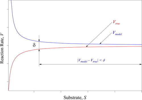
The regularized estimates $V_{max}^{(0)}$ and $K_M^{(0)}$ differ from those usually obtained in the enzyme kinetics [54] by the nonlinear regression techniques. The formulation (28) performs the regularization according to the scheme (6), in which the stabilizer has the norm of Euclidean space, and reconciliation with observations is carried out under the absolute norm. The solution to the problem (28) satisfies the requirements of reducing both the influence of a weak sensitivity of state functions and the effect of measurement errors. Unable to cover this issue in detail, the existence of the weak sensitivity of a hyperbola is illustrated in Figure 6. It demonstrates that there is an observation area in which two different hyperbolas (13) can be matched within a given internal scatter δ. Besides, the existence of significant errors of the estimation was demonstrated in [32], where the least-squares are minimized. All these notes mean that the estimation of the function (13) should be regularized, which will be done here as the formulation (28).

Figure 6. The possibility of matching two different hyperbolas.

Because of the maximum rate $V_{max}$ can be directly determined from the problem (9) – (11), its comparison with the fiducial quantities – in the case of the quasi-steady-state – expresses the adequacy of the reconstruction of the desired vector $\{a,T_{obs}\}$. The values estimated in this way are defined everywhere below as the control quantities, ${\hat{V}}_{max}$ and ${\hat{K}}_M$.

For all the subproblems, the physically justified qualitative information will be used as follows:

1. the positive definiteness of the desired parameters, k_-1, k₁, k₂, S₀, E₀ > 0;

2. the decreasing nature of the functions C and V in the domain $t>t{|}_{V_{max}}$; and

3. the process in the initial stage has a small region, where the maximum reaction rate $V_{max}$ occurs.

All these conditions can be easily implemented within the framework of problems (24) – (27) as the constraints of the minimization problem.

For all the solutions, the numerical control of the determination of the unique element T_obs is provided, which can be done by checking the monotone behaviour of the discrepancy $S(t_i)-S_i^{(\delta )},i=\overline{1,m}$. The uniqueness of the determination of the best element $a^{(\delta )}$is also verified numerically, where the stabilizer minimization and the locally sequential refinement are controlled for chasing the best solution (all details are described below).

9. Experimental data processing

Now, the simulation with the series of the inverse problems, including the locally sequential refinement will be implemented to process two experiments of enzyme kinetics. One of them has a weak dependence on time, and another has a significant dependence on time. All the numerical values will reflect the real values but will have the dimensionless forms according to the remark in Section 5.

The simulation will be divided into two parts of the parameter’s representations – the constant and variable quantities – and will have three steps for each part according to the series of subproblems (24) – (27). Because of this, the reconstruction will express how the simulation errors can be improved in the frame of the sequential regularization of the extension of the object structure.

9.1. Weak time-variable parameters

The case is characterized by the small number of nodes N, for which all features of sought quantities are expressed. The focus will be made on studying the adequate reconstruction of the observation time T_obs. The observation grid dependence over the residuals between the experimental data and model-calculated state is the primary purpose of this subsection. This dependence can express the numerical features of the proposed approach when the sought functions are practically constants.

Let us process the experimental data given in [55]. The samples $S^{(\delta )}$ and $V^{(\delta )}$ are represented in Table 1, Section 1. For this case, the fiducial quantities $V_{max}^{(0)}=0.478$, $K_M^{(0)}$ = 0.077 and the boundary of the consistency corridor ${\hat{\delta }}_{MM}^{(1)}$ = 0.008189 (Section 8) were determined per the solution to the problem (28) (see Table 1, Section 2). Below, the proposed sequence of the regularized solutions is described in detail.

Table 1. The reconstruction $\{a,T_{obs}\}$ for the experimental data [55].

				The constant parameters {k-1, k1, k2, S0, E0} = const						The piecewise linear functions $\{k_{-1},k_1,k_2{\}}_N$ and S0, E0 = const
	The samples		2. Sub- problem (28)	3.1. Subproblem (24)			3.2. Subproblem (26), (27) ${\hat{\delta }}_1=0.0048,{\hat{\delta }}_2=0.0031$			4.1. Subproblem (26), (27), N=9, ${\hat{\delta }}_1={0.1}_{{10}^{-4}},{\hat{\delta }}_2={0.322}_{{10}^{-4}}$			4.2. Subproblem (26), (27), N = 66 ${\hat{\delta }}_1={0.193}_{{10}^{-4}},{\hat{\delta }}_2={0.322}_{{10}^{-4}}$
	$S_{}^{(\delta )}$	$V_{}^{(\delta )}$	$V_{}^{(\delta )}$-V	Tobs	$S_{}^{(\delta )}$- S	$V_{}^{(\delta )}$-V	Tobs	$S_{}^{(\delta )}$- S	$V_{}^{(\delta )}$-V	Tobs	$S_{}^{(\delta )}$- S	$V_{}^{(\delta )}$-V	Tobs	$S_{}^{(\delta )}$- S	$V_{}^{(\delta )}$-V
1	1.078	0.445	−0.001133	1.24229	0.110−^12	0.79410−^2	0.63633	0.002	−0.72710−^3	0.65044	−0.210−^4	−0.32210−^4	0.62546	0.00001	−0.32210−^4
2	0.647	0.435	0.007837	2.42073	0.210−^12	0.13110−^2	1.71704	0.001	−0.30710−^2	1.70809	0.210−^4	0.58310−^5	1.68525	0.00001	0.38010−^5
3	0.431	0.400	−0.005547	3.32786	0.110−^12	0.75610−^2	2.51022	−0.005	0.31110−^2	2.48007	0.110−^5	0.17310−^4	2.45635	0.00001	0.17010−^5
4	0.216	0.345	−0.007382	4.80068	0.110−^12	0.36110−^2	3.66652	−0.005	0.48110−^3	3.67470	0.110−^5	−0.61810−^6	3.62732	0.00000	0.51310−^6
5	0.129	0.305	0.005669	5.99937	0.210−^12	−0.79210−^2	4.41861	0.005	−0.31010−^2	4.51807	0.110−^4	−0.54610−^6	4.46809	0.00000	0.66110−^6
6	0.086	0.260	0.007389	7.11076	0.210−^12	−0.79410−^2	5.19856	0.001	−0.30910−^2	5.24427	0.210−^6	−0.86910−^6	5.18027	0.00000	0.48810−^5
7	0.050	0.180	−0.008189	8.98218	0.510−^12	0.79810−^2	6.67817	−0.005	0.31010−^2	6.43897	0.510−^6	−0.10810−^5	6.39092	−0.00002	0.69910−^5
8	0.040	0.165	0.001581	9.87074	0.210−^12	−0.20410−^2	7.03681	−0.001	0.31010−^2	6.97660	0.210−^6	0.12410−^5	6.91641	0.00002	0.98010−^6
9	0.030	0.140	0.005981	11.1110	0.110−^12	−0.67810−^2	7.70444	0.001	0.31010−^2	7.72943	0.110−^6	−0.14610−^5	7.64525	0.00001	0.90110−^5

9.1.1. The first part: constant parameters

Consider the identification of the constants, k_-1, k₁, k₂, S₀, E₀ = const. Three steps of matching with the observations will be performed according to the serial solutions described in Section 7.

In the first step, requiring the entirely consistent solution to the sample $S^{(\delta )}$, the solution to subproblem (24) with the stabilizer (29) ${\mathrm{\Omega }}_1[a]=k_{-1}^2+k_1^2+k_2^2+S_0^2+E_0^2$(29) is determined. As proved in Section 6, the constant parameters of the Eqs. (9) – (11) are uniquely estimated. By this, no actions are required to divide the invariant family (18), (19).

The reconstruction gives the following estimates:

k_-1= 0.09999, k₁= 1.12380, k₂= 0.17180, S₀= 4.17823, E₀= 3.27367 (${\mathrm{\Omega }}_1$ = 29.48).

The observation grid $T_{obs}\{t_i\}{|}_{i=\overline{1,m}}$, which was reconstructed according to the given volume of the sample m = 9, as well as the residuals with the observations, are shown in Table 1, Section 3.1. The complete composition of the obtained solution is given in the Appendix, Section 1.1 (available in the electronic version of the paper because of the large amount of data). The criteria of the solution adequacy – the worst residuals – have the values ${\rho }_S^{(1,1)}$ = 0.5₁₀−¹², ${\rho }_V^{(1,1)}$ = 0.0079787. The control quantities ${\hat{V}}_{max}^{(1,1)}$ = 0.4536 and ${\hat{K}}_M^{(1,1)}$ = 0.06961 were obtained. Their comparison with the values $V_{max}^{(0)}$and $K_M^{(0)}$shows satisfactory consistency.

In the second step, requiring the regularized minimization of the discrepancies with the samples $S^{(\delta )}$and $V^{(\delta )}$, the solution to subproblem (25) with the stabilizers (29) and (30) ${\mathrm{\Omega }}_2[T_{obs}]=\sum _{i=1}^m{t}_i^2$(30) is considered. This yields the following clarified parameters:

k_-1= 0.21789, k₁= 2.84887, k₂= 0.25702, S₀= 3.03913, E₀= 2.04971 (${\mathrm{\Omega }}_1$ = 21.67, ${\mathrm{\Omega }}_2$ = 229.99).

The regularized observation grid ${\hat{T}}_{obs}{|}_{m=9}$ and other results are given in the Appendix, Section 1.2. The worst residuals ${\rho }_S^{(1,2)}$ = 0.005085, ${\rho }_V^{(1,2)}$ = 0.004086 were obtained. The control quantities ${\hat{V}}_{max}^{(1,2)}$ = 0.4489 and ${\hat{K}}_M^{(1,2)}$ = 0.06539 were determined.

In the third and final step, which required matching into the framework of the consistency corridor, the solutions to subproblems (26) and (27) with the stabilizers (29) and (30) yielded the ultimate constant parameters: (31) $\begin{array}{rl}{k}_{-1}& =0.21217,k_1=2.78724,k_2=0.26260,S_0=2.99964,\\ E_0& =2.01311({\mathrm{\Omega }}_1=20.93,{\mathrm{\Omega }}_2=223.12).\end{array}$(31)

The regularized observation grid $T_{obs}^{(\delta )}{|}_{m=9}$ is shown in Table 1, Section 3.2. The complete composition of the solution is given in Section 1.3 of the Appendix. The consistency corridors ${\hat{\delta }}_1^{(1,3)}=0.0048$ and ${\hat{\delta }}_2^{(1,3)}=0.0031$ were determined. The worst residuals ${\rho }_S^{(1,3)}$= ${\hat{\delta }}_1^{(1,3)}$ and ${\rho }_V^{(1,3)}$= ${\hat{\delta }}_2^{(1,3)}$ were obtained. The control quantities ${\hat{V}}_{max}^{(1,3)}$ = 0.4486 and ${\hat{K}}_M^{(1,3)}$ = 0.06525 were found.

Summarize the results of the reconstruction of the constant parameters.

The residuals, consistency corridors and stabilizers were minimized. It can be seen that all of the transitions under the proposed sequence of the inverse problems improved matching with the samples S^(δ) and V^(δ). The condition ${\hat{\delta }}_{MM}^{(1)}>{\rho }_V^{(1,1)}>{\rho }_S^{(1,2)}>{\rho }_S^{(1,3)}$ reflects the final solution’s improvement. The decrease in the worst residuals expresses the reduction of the simulation error. Such behaviour demonstrates that the proposed regularized solution to the inverse problem series improves the approximation of the experimental data and that the regularized parameters ${\hat{V}}_{max}$ and ${\hat{K}}_M$ are estimated more precisely than the traditional ones $V_{max}^{(0)}$ and $K_M^{(0)}$. At the same time, the lowest values of the stabilizers, ${\mathrm{\Omega }}_1^{(1)}>{\mathrm{\Omega }}_1^{(2)}>{\mathrm{\Omega }}_1^{(3)}$ and ${\mathrm{\Omega }}_2^{(2)}>{\mathrm{\Omega }}_2^{(3)}$ indicate sufficient regularization. In contrast, the least-squares formulation (24) cannot ensure the minimum of the complexity measure.

Thus, it can be concluded that the obtained estimates of the constant parameters adequately characterize the process under study. Though, the next question is of undoubted interest. What will occur if the kinetic parameters are the time-dependent functions? The question is also motivated by the fact that the obtained residuals are higher than the values of observed states. This difference means that the simulation error has a significant value. The improvement of the simulation error requires the widening of the approximation.

9.1.2. The second part: the variable parameters and the local sequential refinement

Consider the identification of the sought parameters as the functions over time using the previously described samples. The piecewise linear functions (32) $\begin{array}{rl}{k}_{-1}& =\frac{{\chi }_{i+1}^{(-1)}-{\chi }_i^{(-1)}}{{\tau }_{i+1}-{\tau }_i}+\frac{{\tau }_{i+1}{\chi }_i^{(-1)}-{\tau }_i{\chi }_{i+1}^{(-1)}}{{\tau }_{i+1}-{\tau }_i}t,{\tau }_i\le t\le {\tau }_{i+1},i=\overline{1,N-1,}\\ k_1& =\frac{{\chi }_{i+1}^{(1)}-{\chi }_i^{(1)}}{{\tau }_{i+1}-{\tau }_i}+\frac{{\tau }_{i+1}{\chi }_i^{(1)}-{\tau }_i{\chi }_{i+1}^{(1)}}{{\tau }_{i+1}-{\tau }_i}t,{\tau }_i\le t\le {\tau }_{i+1},i=\overline{1,N-1},\\ k_2& =\frac{{\chi }_{i+1}^{(2)}-{\chi }_i^{(2)}}{{\tau }_{i+1}-{\tau }_i}+\frac{{\tau }_{i+1}{\chi }_i^{(2)}-{\tau }_i{\chi }_{i+1}^{(2)}}{{\tau }_{i+1}-{\tau }_i}t,{\tau }_i\le t\le {\tau }_{i+1},i=\overline{1,N-1},\end{array}$(32) will approximate the desired quantities k_-1(t), k₁(t), k₂(t). Here $\{{\tau }_i{\}}_{i=\overline{1,N}}$ is the approximation grid, $\mathrm{X}=\{{\chi }_i^{(-1)},{\chi }_i^{(1)},{\chi }_i^{(2)}{\}}_{i=\overline{1,N}}$ denotes the sought nodes of the parameters, and N is the number of the nodes.

The stabilizer is chosen according to the recommendations [34,35] and conclusions of Section 5 as a functional: (33) $\begin{array}{rl}{\mathrm{\Omega }}_3[a]& ={\int }_0^{T_m}{\left(\frac{d{k}_{-1}}{dt}\right)}^{2}dt+{\int }_0^{T_m}{\left(\frac{d{k}_1}{dt}\right)}^{2}dt+{\int }_0^{T_m}{\left(\frac{d{k}_2}{dt}\right)}^{2}dt\\ & +S_0^2+E_0^2+k_{-1}^2{|}_{t=0}+\frac{1}{{k_1^2|}_{t=0}},\end{array}$(33) where T_m denotes the final time of the observation. The functional Ω₃ expresses the conditions of the segregation of the sought parameters from the invariant subset (18), (19). Its minimization facilitates the unique reconstruction of the variable kinetics parameters (see Section 6).

The measure of the solution complexity $\mathfrak{M}={\int }_0^{T_m}{\left(\frac{d{k}_{-1}}{dt}\right)}^{2}dt+{\int }_0^{T_m}{\left(\frac{d{k}_1}{dt}\right)}^{2}dt+{\int }_0^{T_m}{\left(\frac{d{k}_2}{dt}\right)}^{2}dt$ is introduced to control the reconstruction quality for all the cases considered below. The measure will express the solution deviations from the constant values.

For all the cases considered below the differences are not significant between the observation grid $T_{obs}\{t_i\}{|}_{i=\overline{1,m}}$ obtained in the framework of three solutions to the serial subproblems (24) – (27). Therefore, only the final results are represented.

The first step of the reconstruction is the identification of the node’s set $\mathrm{X}=\{{\chi }_i^{(-1)},{\chi }_i^{(1)},{\chi }_i^{(2)}{\}}_{i=\overline{1,N}}$, the volume of which has a small size, N ≤ m. The solutions to subproblems (26), (27) and the locally sequential refinement for partitioning the estimation interval with N = m, where m = 9, yielded the estimates S₀ = 3.00293, E₀ = 2.01037. The final observation grid $T_{obs}^{(\delta )}{|}_{m=9}$ is presented in Table 1, Section 4.1. The identified approximation nodes $\{{\chi }_i^{(-1)},{\chi }_i^{(1)},{\chi }_i^{(2)}{\}}_{i=\overline{1,9}}$ are given in the Appendix, Section 1.5. The measure $\mathfrak{M}{|}_{N=9}=0.071665$ and the control quantities ${\hat{V}}_{max}^{(1,4)}$ = 0.45012, ${\hat{K}}_M^{(1,4)}$ = 0.06842 were obtained.

This step demonstrates that the residuals with the observations are improved, ${\rho }_S^{(1,4)}$ = 2.39₁₀−⁵, ${\rho }_V^{(1,4)}$ = 3.22₁₀−⁵. However, the number of nodes N = 9 does not express satisfactory approximation. Because of this, the magnification of the number N should be continued.

The second step of the reconstruction is the sequential increase of node number N. The locally sequential refinement of the solutions to the subproblems (26), (27) was executed under the stabilizers (30) and (32). The consistency corridors ${\hat{\delta }}_1^{(1,5)}={1.93}_{{10}^{-5}},{\hat{\delta }}_2^{(1,5)}$ = 3.22₁₀−⁵ were found. The satisfactory approximation of the sought functions was started from the value N = 66 (Table 1, Section 4.2). The desired initial states S₀ = 2.9913, E₀ = 2.0066 were determined. The reconstructed nodes $\{{\chi }_i^{(-1)},{\chi }_i^{(1)},{\chi }_i^{(2)}{\}}_{i=\overline{1,9}}$ are shown in the Appendix, Section 1.6. The measure $\mathfrak{M}{|}_{N=66}=0.0136$, the worst residuals ${\rho }_S^{(1,5)}$= ${\hat{\delta }}_1^{(1,5)}$, ${\rho }_V^{(1,5)}$ = ${\hat{\delta }}_2^{(1,5)}$ and the control quantities ${\hat{V}}_{max}^{(1,5)}$ = 0.45102, ${\hat{K}}_M^{(1,5)}=0.06846$ were obtained.

Summarize the results of the reconstruction of the variable parameters k_-1(t), k₁(t), k₂(t).

The serial regularized solutions depict decreasing the measure of the solution complexity, $\mathfrak{M}{|}_{N_{i-1}}$> $\mathfrak{M}{|}_{N_i},i=\overline{2,66}$ (Table 2). Such behaviour means that the stabilization of the desired solution is satisfactory. The values of the obtained residuals differ from the residuals of the previous case with the constant parameters (subsection 9.1.1). Their improvements are of more than two orders of magnitude. At the same time, the deviations of the variable parameters k_-1(t), k₁(t), k₂(t) from the constants in (31) are not significant. The observation grid $T_{obs}^{(\delta )}{|}_{m=9}$ and the initial states S₀, E_0, which were estimated for the piecewise linear approximation, differ insignificantly from the values, which were obtained for the constants (Table 1, Sections 3 and 4). The estimates $V_{max}^{(0)}$ and $K_M^{(0)}$ differ from the values ${\hat{V}}_{max}^{(1,5)}$ and ${\hat{K}}_M^{(1,5)}$by about 4.85% and 11.18% consequently.

Table 2. The measure of the solution complexity and matching with the observations for the different number of nodes N, experimental data [55], and subproblem (26), (27).

The number of nodes, N	9	25	34	44	50	60	66
${\displaystyle \int {\left({\displaystyle \frac{d{k}_1}{dt}}\right)}^{2}dt+\int {\left({\displaystyle \frac{d{k}_{-1}}{dt}}\right)}^{2}dt+\int {\left({\displaystyle \frac{d{k}_2}{dt}}\right)}^{2}dt}$	0.071665	0.051513	0.051046	0.048140	0.039877	0.025544	0.013569
$\underset{1\le i\le m}{\text{max}}|S{(t_i)|}_{a^{(\delta )}}-S_i^{(\delta )}|$	0.2390810−^4	0.1876210−^4	0.22710−^10	0.22710−^10	0.22710−^10	0.1784910−^4	0.1927410−^4
${\displaystyle \sum _{i=1}^m[S{(t_i)|}_a-S_i^{(\delta )}{]}^2}$	0.9846610−^5	0.1035210−^4	0.11110−^10	0.11110−^10	0.11110−^10	0.9313410−^5	0.1074910−^4
$\underset{1\le i\le m}{\text{max}}|V{(t_i)|}_{a^{(\delta )}}-V_i^{(\delta )}|$	0.3211110−^4	0.1751710−^4	0.11410−^4	0.77510−^5	0.13010−^4	0.1987810−^4	0.3212610−^4
${\displaystyle \sum _{i=1}^m[V{(t_i)|}_{\hat{a}}-V_i^{(\delta )}{]}^2}$	0.1234610−^4	0.1093110−^4	0.36310−^5	0.31310−^5	0.64110−^5	0.1116010−^4	0.1157210−^4

All the criteria of the adequate solution such as the absence of numerical oscillations in the general and local sense, the minimum of the residuals ${\rho }_{S,V}^{}$, and decreasing the complexity measure M are satisfied. It is remarkable for the proposed approach (Section 4), that the transition from the approximation nodes N = 6 to N = 66 has not changed the estimations significantly despite the limited size of the sample.

Thus, the proposed solutions to the series of the inverse problems (24) – (27) and the locally sequential refinement can satisfactorily reconstruct not only the unknown parameters but also the observation grid $T_{obs}\{t_i\}{|}_{i=\overline{1,m}}$. The control and fiducial quantities obtained by the different methods are close to the estimates. The reconciliation confirms the reconstruction adequacy. This conclusion is also confirmed by the fact that the time-dependent parameters differ slightly from the previously reconstructed constant parameters. That is, having extended the approximation meaningfully, the estimates have not changed significantly. For enzyme kinetics, it is indicative that the transition to the variable kinetic parameters k_-1(t), k₁(t), k₂(t) significantly improves the approximation of the observations $V^{(\delta )}$. The obtained results demonstrate the general character of the object under study.

9.2. Reconstruction of complex dependencies

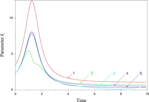
Having obtained confirmation in the previous subsection that the observation grid was adequately reconstructed, we turn to the desired parameters k_-1, k₁, k₂ with the strong dependence over time. The identification of the kinetic parameters is performed for the case of a large number of the nodes N, which is required to approximate the sought functions satisfactorily. Of course, such a case has significantly more uncertainties than the previous case. It is attractive to determine the best solution among others who are close in the residuals but differ significantly in nature.

• Let us process the experimental data [56]. The samples $S^{(\delta )}$ and $V^{(\delta )}$ are represented in Table 3, Section 1. For them, the solution to the problem (28) yields the regularized fiducial quantities $V_{max}^{(0)}$ = 1.2967 and $K_M^{(0)}$ = 6.3558. The consistency corridor was determined ${\hat{\delta }}_{MM}^{(2)}$ = 0.1888 (Table 3, Section 2).

• It is indicative that the value ${\hat{\delta }}_{MM}^{(2)}$ is more than 10% regarding the maximum rate of $V_{max}$. The values $V_{max}^{(obs)}$ = 0.997, $K_M^{(obs)}$ = 4.467 are determined from experimental data. A comparison with the values $V_{max}^{(0)}$and $K_M^{(0)}$ highlights that the application of the Michaelis–Menten function gives significant simulation errors. Therefore, the approximation of the observations by the function (13) is unsatisfactory. This fact was noted earlier in [56], where the fitting of the experimental data by the function (13) was recognized to be unsuitable for use. The reason is the distinction of the observed process from the quasi-steady-state. Because of this, the simulation expansion is required. In [56], it was another hyperbola-kind function. The simulation with the inverse problems (Section 7) will identify the kinetic parameters without any postulation of their functional kind.

Table 3. The reconstruction $\{a,T_{obs}\}$ for the experimental data [56].

				3. The piecewise constant functions $\{k_{-1},k_1,k_2{\}}_{N=3}$ and S0, E0=const, subproblem (26), (27) ${\hat{\delta }}_1=0.0003,{\hat{\delta }}_2=0.129$							4. The piecewise linear functions $\{k_{-1},k_1,k_2{\}}_N$ and S0, E0 = const
	1. The samples		2. Subproblem (28)	4.1. Subproblem (24), N = 6		4.2. Subproblem (24), N = 11			4.3. Subproblem (24), N = 31			4.4. Subproblem (24), N = 51			4.5. Subproblem (26), (27), N = 176, ${\hat{\delta }}_1=0.0005,{\hat{\delta }}_2=0.001$
	$S_{}^{(\delta )}$	$V_{}^{(\delta )}$	$V_{}^{(\delta )}$-V	Tobs	$S_{}^{(\delta )}$- S	$V_{}^{(\delta )}$-V	Tobs	$V_{}^{(\delta )}$-V	Tobs	$V_{}^{(\delta )}$-V	Tobs	$V_{}^{(\delta )}$-V	Tobs	$V_{}^{(\delta )}$-V	Tobs	$S_{}^{(\delta )}$- S	$V_{}^{(\delta )}$-V
1	67.60	0.997	−0.18826	0.00641	0.29710−^3	−0.16410−^2	1.1965	0.69610−^3	1.1952	0.47010−^3	1.2003	−0.11310−^4	1.2003	−0.50210−^5	1.190	−0.00038	−0.10910−^2
2	29.514	0.990	−0.07694	32.31156	−0.34210−^3	−0.126	40.737	0.10810−^2	40.725	−0.15310−^3	39.987	−0.20110−^5	39.988	−0.18410−^5	39.513	0.00045	0.10910−^2
3	12.88	0.969	0.10075	48.39442	0.15010−^3	0.22210−^1	57.511	−0.48710−^2	57.534	−0.17510−^3	57.179	0.20510−^7	57.181	0.15110−^5	56.673	−0.00049	−0.10910−2
4	7.940	0.909	0.18880	54.17396	0.19910−^3	0.97910−^1	62.845	0.39610−^2	62.882	0.44410−^4	62.517	−0.12210−^6	62.518	−0.91110−^6	62.042	−0.00049	0.11210−3
5	5.750	0.760	0.14409	57.21288	0.18710−^3	0.49810−^1	65.550	0.10310−^3	65.589	−0.18310−^3	65.240	−0.10510−^5	65.242	−0.77510−^5	64.858	−0.00050	0.42210−4
6	4.467	0.500	−0.03520	59.27994	0.15610−^3	−0.128	67.981	0.12810−^3	68.026	0.14310−^3	67.685	0.22110−^6	67.686	−0.20410−^5	67.161	−0.00051	−0.25910−3
7	2.884	0.240	−0.16474	65.01216	−0.29710−^3	−0.51310−^3	74.305	0.87410−^4	74.331	−0.19610−^3	74.382	−0.88310−^7	74.312	0.33910−^5	72.349	−0.00050	−0.84110−^4
8	1.748	0.0909	−0.18880	78.77295	−0.30810−^3	0.80110−^2	81.320	0.69010−^4	81.273	0.60110−^4	80.995	0.17610−^5	81.145	0.26310−^6	80.565	−0.00050	−0.49910−^4
9	0.794	0.0306	−0.11340	96.59349	−0.24410−^3	−0.10210−^1	124.548	0.15110−^2	162.975	−0.42710−^5	170.693	0.13810−^6	174.821	−0.11710−^7	99.382	−0.00050	0.13010−^3
10	0.350	0.0099	−0.57779	114.2763	−0.14510−^3	−0.88210−^2	147.628	−0.30810−^2	182.562	−0.15110−^3	198.263	−0.26910−^5	203.229	−0.44610−^6	124.183	−0.00050	0.32910−^5
11	0.100	0.00315	−0.01694	140.6856	−0.54210−^4	−0.23210−^2	182.617	−0.58510−^3	227.377	0.26310−^3	241.129	0.23210−^6	245.464	0.25210−^6	157.756	0.00021	0.10810−^2

It is important to note that the experimental data [56], unlike the previous ones, has the observations for the key areas of the state functions. Both the region of the maximum rate $V_{max}$ and the final stage of the process are these essential areas. The observations of the similar parts of the direct problem solution facilitate the complete control of the estimation adequacy. Ignoring observations in these areas will distort the process representation over the entire period of its existence. Consequently, the properties of the direct solution will be extensively used below.

9.2.1. The first part: constant parameters

Consider the reconstruction of the constants k_-1, k₁, k₂, S₀, E₀ = const. Similar to subsection 9.1.1, three inverse problems (Section 7) will be solved.

In the first step, the solution to subproblem (24) with the stabilizer (29) yields the following sought parameters: $k_{-1}=26.651,k_1=4.366,k_2=0.685,S_0=77.452,E_0=\mathrm{1.877.}$

The results, which reflect the overall solution, are given in the Appendix, Section 2.1. The worst residuals ${\rho }_S^{(2,1)}$ = 0.45₁₀−⁹ and ${\rho }_V^{(2,1)}$ = 0.19057 were obtained. The control quantities ${\hat{V}}_{max}^{(2,1)}$ = 1.1875 and ${\hat{K}}_M^{(2,1)}$ = 5.3615 were determined. A comparison between the control and fiducial quantities shows poor consistency.

In the second step, solving subproblem (25) with the stabilizers (29) and (30) clarifies the parameters as follows: $k_{-1}=26.65097,k_1=4.367905,k_2=0.68387,S_0=77.45812,E_0=\mathrm{1.88003.}$

All other estimates are shown in the Appendix, Section 2.2. The worst residuals ${\rho }_S^{(2,2)}$ = 0.0028 and ${\rho }_V^{(2,2)}$ = 0.19073 were obtained. The control quantities ${\hat{V}}_{max}^{(2,2)}$ = 1.1875 and ${\hat{K}}_M^{(2,2)}$ = 5.3592 were gained.

In the third and final step, the solutions to problems (26) and (27) using the stabilizers (29) and (30) and the boundaries of the consistency corridor ${\hat{\delta }}_1^{(2,3)}=0.1,{\hat{\delta }}_2^{(2,3)}=0.185$ improve the estimation. The worst residuals have become smaller than in the previous step: ${\rho }_S^{(2,3)}$ = 0.10004 and ${\rho }_V^{(2,3)}$ = 0.18471. Finally, the constant parameters were estimated as follows: $k_{-1}=22.93453,k_1=3.92488,k_2=0.76917,S_0=70.30741,E_0=\mathrm{1.65229.}$

Other obtained results are given in the Appendix, Section 2.3. The solution to the direct problem (9) – (11) yields the control quantities ${\hat{V}}_{max}^{(2,3)}$ = 1.1683 and ${\hat{K}}_M^{(2,3)}$ = 5.1246.

All of the results of this part of the simulation demonstrate that in the framework of the constant kinetic parameters, the consistency with the observations remains weak, and the best residual ${\rho }_{S,V}^{(2,3)}$ differs slightly from the value ${\hat{\delta }}_{MM}^{(2)}$. From the adequacy viewpoint, it is critical that the behaviour of the identified function V(t) in the region with the maximum rate $V_{max}$ differs meaningfully from the observations (see the Appendix, Sections 2.1–2.3).

Thus, the simulation of the kinetic process with the constant kinetic parameters is unsatisfactory.

9.2.2. The second part: the variable parameters and the local sequential refinement

The dependence of the sought parameters on time is considered as the primary condition to improve the simulation accuracy. The approximation will be sequentially extended from simple to complicated functional representations. The previously identified properties of the object in question are the basis of the required extension.

The first step of the simulation accounts for the existence of three areas of the worst reconciliation obtained in the previous subsection (see the Appendix, Section 2.3). According to these areas of unsatisfactory consistency, and following the recommendations of Section 4, the sought parameters k_-1(t), k₁(t), k₂(t) were approximated by three piecewise constant functions, for which the variability intervals are 0 < t₁ ≤ 50, 50 < t₂ < 65, t₃ ≥ 65. The stabilizer was as follows: ${\mathrm{\Omega }}_4[a]={\int }_0^{T_m}(k_{-1}^2+k_1^2+k_2^2)dt+S_0^2+E_0^2.$

For this case of partitioning, the proposed sequence (24) – (27) facilitates identifying the parameters S₀ = 68.86097, E₀ = 1.63189. All other results are shown in Table 3, Section 3, and the Appendix, Section 2.4. The control quantities are ${\hat{V}}_{max}^{(2,4)}$ = 1.2107 and ${\hat{K}}_M^{(2,4)}$ = 4.1539. The consistency corridors turn out to be ${\hat{\delta }}_1^{(2,4)}=0.00035,{\hat{\delta }}_2^{(2,4)}=0.129$. The estimates express the improvement in the consistency, for which the worst residuals ${\rho }_S^{(2,4)}$ = 0.00034, ${\rho }_V^{(2,4)}$ = 0.12873 are obtained. Because of this, the approximation extension is the correct way to decrease the simulation error.

The second step is the approximant change to the piecewise linear functions (32). The initial number of the nodes was N = 6 (Table 3, Section 4). The other initial values were selected from the previous step. The stabilizers (33) and (30) were used. The solution convergence was controlled according to the level of the change in the complexity measure M (Table 4).

Table 4. The measure of the solution complexity and matching with the observations for the different number of nodes N, experimental data [56], and subproblem (24).

The number of nodes N	6	11	31	51	71	91	101	176
${\displaystyle \int {\left({\displaystyle \frac{d{k}_1}{dt}}\right)}^{2}dt+\int {\left({\displaystyle \frac{d{k}_{-1}}{dt}}\right)}^{2}dt+\int {\left({\displaystyle \frac{d{k}_2}{dt}}\right)}^{2}dt}$	521.5505	309.388	238.5441	134.4317	60.3046	24.3784	22.0499	9.9679
$\underset{1\le i\le m}{\text{max}}|S{(t_i)|}_{a^{(\delta )}}-S_i^{(\delta )}|$	0.22710−^10	0.45410−^9	0.22710−^10	0.22710−^10	0.22710−^10	0.22710−^10	0.22710−^10	0.50510−^3
${\displaystyle \sum _{i=1}^m[S{(t_i)|}_a-S_i^{(\delta )}{]}^2}$	0.10410−^10	0.17910−^9	0.11110−^10	0.11110−^10	0.11110−^10	0.11110−^10	0.11110−^10	0.46610−^3
$\underset{1\le i\le m}{\text{max}}|V{(t_i)|}_{a^{(\delta )}}-V_i^{(\delta )}|$	0.48710−^2	0.47010−^3	0.11410−^4	0.77510−^5	0.13010−^4	0.33610−^4	0.44110−^4	0.10910−^2
${\displaystyle \sum _{i=1}^m[V{(t_i)|}_{\hat{a}}-V_i^{(\delta )}{]}^2}$	0.22110−^2	0.22010−^3	0.36310−^5	0.31310−^5	0.64110−^5	0.15710−^4	0.14610−^4	0.66410−^3

The third step of the reconstruction is the sequential increase of node number N. The locally sequential refinement has played a crucial role in eliminating the loss of numerical stability during the identification. Namely, the principle of reconstructing only the parts of each desired function, and not immediately identifying them as a whole, ensures attracting a large number of the discretization nodes. By this and following the regularization principle, the solution was built as smooth as possible for each N. Here, the weak consistency with the samples is typical. Further, the residuals were minimized to determine the best consistency corridor. Finally, the particularization of the desired quantities was carried out into the framework of the consistency corridor.

For the experimental data under study, the node number of satisfactory approximation was started from the value N = 165. For this value, the consistency corridors ${\hat{\delta }}_1^{(2,5)}$ = 0.05 and ${\hat{\delta }}_{12}^{(2,5)}$ = 0.03 were determined to identify the smoothest kinetic parameters (subsection 2.10 of the Appendix). Based on this solution, the reconstruction was accomplished to achieve minimal residuals with the samples (subsection 2.11 of the Appendix). The regularized reconstruction has reflected the pulsation character of the kinetic parameters. After this, the pulsation detailing was performed (Figure 12 and subsection 2.12 of the Appendix). Compared to the previous reconstruction, the latter solution has improved the monotonous behaviour of C and V functions.

The final node number was N = 176. The minimal consistency corridors ${\hat{\delta }}_1^{(2,6)}=0.0005,{\hat{\delta }}_2^{(2,6)}=0.001$ were determined. The initial states S₀ = 70.101, E₀ = 1.463 were identified. The control quantities ${\hat{V}}_{max}^{(2,5)}$ = 1.004, ${\hat{K}}_M^{(2,5)}$ = 4.4766 were found. The reconstructed grid $T_{obs}^{(\delta )}{|}_{m=11}$ is given in Table 3, Section 4.5. The sought nodes $\{{\chi }_i^{(-1)},{\chi }_i^{(1)},{\chi }_i^{(2)}{\}}_{i=\overline{1,N}}$ for the various N are presented in subsections 2.5–2.12 of the Appendix.

All the above-listed results express the unique and stable reconstruction of four functions k_-1(t), k₁(t), k₂(t), T_obs, whose approximations required 539 nodes and for which only two samples with a total volume of 22 points were used.

9.2.3. The features of the reconstruction

In Figures 7–9, the changes of the functions k_-1(t), k₁(t), k₂(t) are depicted during the locally sequential refinement. Their sequential transformations show that exchanging from the simple to the complex representations has a strictly defined final form (Figures 10). The direct problem solution with identified parameters expresses all the features of the kinetic under study (Figures 11 and 12). The constants and the final representations of the kinetic parameters are the interrelated forms. The estimates are not arbitrary or random (compared to Figures 10 and 13) and do not contain oscillating components (compared to Figures 10 and 14).

Figure 7. The estimation of the parameter k_-1 for the various nodes N (its value is indicated on the curves).

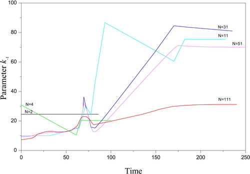
Figure 8. The estimation of the parameter k₁ for the various nodes N (its value is indicated on the curves).

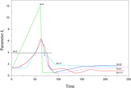
Figure 9. The estimation of the parameter k₂ for the various nodes N (its value is indicated on the curves).

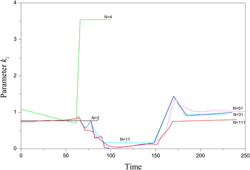
Figure 10. The reconstructed kinetic parameters, N = 176 (the experimental data [56]): 1 – the parameter k_-1, 2 – the parameter k₁, 3 – the parameter k₂.

Figure 11. The reconstructed functions, N = 176 (the experimental data [56]): 1 – C, 2 – V.

Figure 12. The dependence V(S): 1 – the experimental data [56], 2 – the regularized solution, N = 176, 3 – the Michaelis-Menten function with the parameters $V_{max}^{(0)}$ and $K_M^{(0)}$.

Figure 13. The exclusion of the locally sequential refinement from the sequence (24) – (27), N = 11.

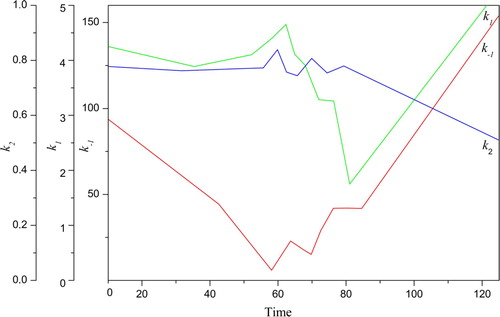
Figure 14. The local refinement without the regularization, N = 71.

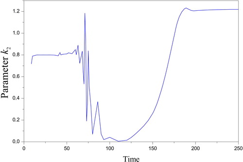
The essential part of the reconstruction was the control over the behavior of the direct problem solutions C(t) and V(t). It is supposed that the functions C(t) and V(t) should be increasing at the range $t<t{|}_{V_{max}}$, and should be decreasing at the range $t>t{|}_{V_{max}}$. The local disturbances of the solution monotonicity have occurred during the increase of the nodes number N (Figure 15). The control has determined the character and behaviour of the sought parameters significantly. In particular, the staircase character of the parameters k_-1(t), k₁(t), k₂(t) at the initial stage was revealed precisely due to this control.

Figure 15. The magnification of nodes and the local violation of the function V monotonous: a) N = 95; b) N = 131; c) N = 161; d) N = 95; e) N = 131; f) N = 151.

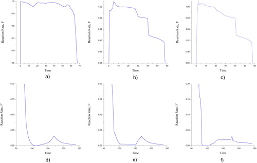
Especially underline that another essential part of the reconstruction stabilization was the third subproblem in the sequence of the solutions (Section 7). It facilitates matching into the framework of the consistency corridors. Satisfying the latter condition provides the effective restriction of numerical oscillations. The solution was determined on the boundaries of these corridors per the regularization feature [42]. Because of this, only the minimization of residuals with samples, including its regularized formulation, for example (24), in principle, cannot give the satisfactory detailing of the sought functions (see subsubsection 9.2.4).

Also, note that even regularized estimates $V_{max}^{(0)}$ and $K_M^{(0)}$, described in subsection 5.2 as the commonly used enzyme model, cannot adequately reflect the area with the maximum reaction rate for the experimental data under the study. To explain the difference between the fiducial and control quantities, the dependence of V(S) should be considered. Figure 12 expresses the cause of the difference. It is the piecewise monotonic behavior of the function V(S). Fitting by the smooth hyperbola (13) gives rise to the insufficient approximation (Figure 12) and, consequently, the discrepancies with the observations have high values. All the obtained solutions highlight that the traditional approach gives rise to the overestimation, $V_{max}^{(0)}>{\hat{V}}_{max}$. The comparison with the inverse problem solution, which was obtained in [32] by the least-squares method, demonstrates the advantage of the mandatory regularization having the pinpoint accuracy of the regularized estimates $V_{max}^{(0)}$ and $K_M^{(0)}$ (see Figure 12).

A positive feature of the regularized reconstruction is a gradual decrease in the complexity measure $\mathfrak{M}$ (Table 3). Such behaviour indicates the regularity of functional expansion. The use of other starting values of sought quantities, as well as the forced change of any of them during the reconstruction, reduced the measure $\mathfrak{M}$ only when the initial values $S_0,E_0,k_{-1}{|}_{t=0},k_1{|}_{t=0}$ were excluded from the stabilizer (32). However, this exclusion gives rise to the intense smoothing of the solution.

9.2.4. The significance of the sequential refinement procedures

Let us demonstrate the significance of each option of the proposed sequence of regularized solutions.

For the first option – without the locally sequential reconstruction – only the problems (26) and (27) were solved at once for the whole nodes $\{{\chi }_i^{(-1)},{\chi }_i^{(1)},{\chi }_i^{(2)}{\}}_{i=\overline{1,11}}$ with the small discretization, N = 11. The results are presented in Figure 13. As can be seen, the arbitrary forms of the sought functions were obtained. However, for this case, the solution regularization and matching with the observations were fulfilled, and the discrepancies with the observations were rather low, $\underset{1\le i\le 11}{\text{max}}|S{(t_i)|}_{a^{(\delta )}}-S_i^{(\delta )}|={{2.27}_{10}}^{-9},\underset{1\le i\le 11}{\text{max}}|V{(t_i)|}_{a^{(\delta )}}-V_i^{(\delta )}|={{2.55}_{10}}^{-2}.$ These values demonstrate that the object in question has a typical feature of ill-posed problems. Here, the small discrepancies between the state functions and their observations correspond to the significant variations of the sought parameters. If the locally sequential refinement of the reconstruction is not performed, then the filtration of arbitrary elements is absent.

For the second option – without the general regularization – the solution to subproblem (24) with the refinement into the local interval 60 ≤ t ≤ 80 was determined, where the stabilizer Ω₃[a] was not used, and the sought functions {k_-1(t), k₁(t), k₂(t)}_N=71 were estimated by the minimization of the least-squares. As can be seen in Figure 14, the numerical instability occurs if the least-squares are minimized without the solution restriction. The stability absence demonstrates the principal role of the stabilizer and the local refinement.

9.2.5. The dependence on the noise level

In the case of unknown noise level, it is crucial to investigate its effect on the reconstruction. Here, two factors matter: i) the sensitivity of solving the direct problem to changes in the desired parameters, and ii) the numerical stability performed by the reconstruction method. If the analysis is limited to the particular cases, then numerical simulation of observations with increasing measurement errors is sufficient.

Let us carry out such modelling for the observations of the states S and V, which are determined from the solution to the direct problem (9) – (11) with the reference parameters {$a^{(\delta )}$, $T_{obs}^{(\delta )}$} reconstructed in subsection 9.2.2. The samples $S^{(\delta )}$ and $V^{(\delta )}$ will be simulated according to Eqs. (14), where ${\epsilon }_{1,2}$ is the random functions with a normal distribution. The observations with 1%, 5% and 10% noise from the current value of the observed state and the volume m = 11 are shown in Figure 16. For them, the approach described in Sections 4 and 7 was applied. The results are represented in Figure 17.

Figure 16. The sample simulation with the noise level 1%, 5% and 10%.

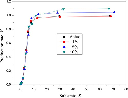
Figure 17. The reconstruction with the noise simulation: 1 – the actual parameter, 2 – the noise level 1%, 3 – the noise level 5%, 4 – the noise level 10%.

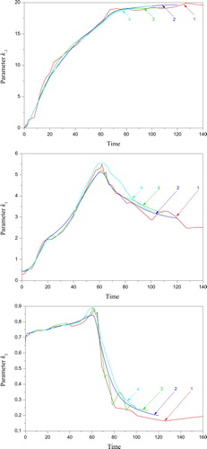
The reconstruction generally reflects the previously noted smoothing property of the solution when the consistency corridor ${\hat{\delta }}_{1,2}$ is extended. For the noise 1% and 5%, the desired vector $\{a,T_{obs}\}$ was identified for arbitrarily given initial values both relative to the parameters $a^{(\delta )}$ and the grid $T_{obs}^{(\delta )}$. For the small noise, δ ≤1%, the reconstruction by the proposed approach gives the functions, which differs slightly from the reference quantities. For the noise 5% and 10%, the details of the reference functions are smoothed, but the general functional properties – the regions of the growth and decrease, minimum and maximum values – are saved. However, for the noise 10%, an arbitrary set of the initial grid $T_{obs}^{(\delta )}$ led to zero values of its nodes, $t_i=0,i=\overline{1,11}$. The solution convergence was restored if the initial values of the sought grid $T_{obs}^{(\delta )}$ were chosen near the reference values. In practice, this means that for increased noise, the simultaneous identification of the parameters a and the nodes $T_{obs}$ had significant difficulties in meeting the convergence conditions. It will be executed when the nodes $T_{obs}$ are approximately known. Such a solution behaviour underlines the significance of both a level of noise and observation conditions in the problem formulation. It is also noteworthy that the reconstruction with increased noise leads to a highly biased estimate of the right boundary $t_m$ of the observation interval.

Thus, the simulation with the series of the inverse problems, including the locally sequential refinement, was successfully applied in the case of acting at once all the known features of ill-posed problems such as nonuniqueness, nonstability, poor sensitivities, and noise action. If the sufficient domain restrictions are met, then the solution to the inverse problem can be determined within the framework of significant uncertainties. The simulation with inverse problems facilitates not only identifying all of the kinetic parameters but also clarifying the observation conditions.

10. Conclusions

The main results of the investigation are as follows.

Comprehensive information on an object’s properties can be extracted from a small sample.

If a sample has a limited size, then the basis of the stable identification of a large number of unknowns is the locally sequential refinement of the approximation of desired quantities. The locally sequential refinement requires the maximum restrictions of the feasible region in general.

The object in question has all the attributes of the ill-posed problem, namely, the violation of the one-to-one correspondence, the oscillations of the numerical calculations and the weak sensitivity to the local variation of the object’s states. However, the unique and stable solution was determined, and the reconstruction of the complicated dependencies using the small volume of observations was carried out.

The proposed regularization under separate matching with observations facilitates the stable estimation, adequate reconciliation with samples, and determination of the consistency corridor of the solutions with the given observations. The essential part of the reconstruction is adequate accounting for the multiple characters of samples as well as matching the solution with the noise level separately for each element of the observation set. The regularization of the complex functional dependencies without the locally sequential refinement gives rise to arbitrary solutions. The stabilizers were successfully used in fulfilling the solution restrictions throughout the variable domain space, and the locally sequential refinement showed the effectiveness in eliminating the local violations during the increase of the discretization nodes.

Any additional information, including the conditions of the unique solution to the inverse problem, can be involved in the regularization to facilitate the improvement of the estimation. The proposed regularization can take into account any changes during the simulation, such as the type of the approximation, the kind of the model used, the nature of the restrictions imposed and other changes.

The expansion of the desired solution with several unknowns leads to the formulation of the sequence of the inverse problems. Their choice should be based on the principle of ‘from simple to complex and extended’. The exclusion of restrictions from any level of the simulation leads to arbitrary solutions.

The effectiveness of the proposed approach was compared with the traditional processing of enzyme kinetics experiments. In one case, the satisfactory reconciliation was obtained, and in another, there was a significant difference with the results of the hyperbola’s estimation. The difference has appeared because the Michaelis–Menten function is not applicable to objects with variable kinetic parameters. For all the considered experimental data, the transition to the dependencies of kinetic parameters over time improved the consistency with the observations.

The solution to the inverse problem provides important additional information regarding the features of the enzyme kinetics. The pair $\{V_{max},K_M\}$ were reconstructed more precisely than the ones obtained by the Michaelis–Menten function. For the inverse problem, the mandatory observations in the quasi-stationary region, which are required for the application of the Michaelis–Menten function, do not matter in principle. Moreover, the most preferred observations are fulfilled in the areas, where the reactions turn out to be essentially nonstationary. The obtained solutions express the necessary components of the experimental data, which can offer the best estimation of the kinetic parameters.

Further investigations will be directed to estimate the parameters of the Verhulst equation, commonly known in biomathematics. The simulation with inverse problems will facilitate revealing novel features of the growth processes.

Acknowledgements

The author would like to thank the reviewers, whose attention and comments have substantially improved the presentation of the results and have supported the publication.

Disclosure statement

No potential conflict of interest was reported by the author(s).

References

- Lavrentiev MM, Romanov VG, Vasiliev VG. Multidimensional inverse problems for differential equations. New York: Springer-Verlag; 1970.
- Glasko VB. Inverse problems of mathematical physics. New York: American Institute of Physics; 1988.
- Groetsch CW. Inverse problems in the mathematical sciences. Braunschweig Wiesbaden: Vieweg; 1993.
- Engl HW, Hanke M, Neubauer A. Regularization of inverse problems. Dordrecht: Kluwer Academic Publishers; 2000.
- Tarantola A. Inverse problem theory and methods for model parameter estimation. Philadelphia: SIAM; 2005.
- Ramm A. Inverse problems. mathematical and analytical techniques with applications to engineering. Boston: Springer; 2005.
- Isakov V. Inverse problems for partial differential equations. 2nd ed New York: Springer; 2006.
- Kirsch A. An introduction to the mathematical theory of inverse problems. New York: Springer; 2011.
- Romanovskii MR. Solution of inverse problems with an unknown model of the process. J Eng Phys. 1983;45(3):1076–1082. doi: 10.1007/BF00826508
- Tikhonov AN, Arsenin V. Solutions of ill-posed problems. New York: Halsted Press; 1977.
- Romanovskii MR. Recreating the structure of an object as a whole by using the properties of one part. J Eng Phys. 1991;60(6):800–805. doi: 10.1007/BF00871524
- Shaw FS. An introduction to relaxation methods. New York: Dover Publications, Inc.; 1953.
- Ortega JM, Rheinboldt WC. Iterative solution of nonlinear equations in several variables. Philadelphia: SIAM; 2000.
- Trottenberg U, Oosterlee CW, Schüller A. Multigrid. London: Academic Press; 2001.
- Minoux M. Mathematical programming: theory and algorithms. New York: Wiley-Interscience Publication; 2008.
- Ascher UM, Lin P. Sequential regularization methods for higher index DAEs with constraint singularities: The linear index-2 case. SIAM J Numer Anal. 1995;33(5):1921–1940. doi: 10.1137/S0036142993253254
- Lin P. A sequential regularization method for time-dependent incompressible Navier-Stokes equations. SIAM J Numer Anal. 1996;34(3):1051–1071. doi: 10.1137/S0036142994270521
- Bertsimas D, Brown DB, Caramanis C. Theory and Applications of robust optimization. SIAM Rev. 2011;53(3):464–501. doi: 10.1137/080734510
- García J, Peña A. Robust optimization: Concepts and Applications. In: Nature-inspired methods for Stochastic, robust and dynamic optimization. Intechopen; 2018. DOI:10.5772/intechopen.75381
- Alpaydin E. Introduction to machine learning. Cambridge: The MIT Press; 2004.
- Shawe-Taylor J, Cristianini N. Kernel methods for pattern analysis. University Press: Cambridge; 2004.
- Mohri M, Rostamizadeh A, Talwalkar A. Foundations of machine learning. Cambridge: The MIT Press; 2012.
- Mishra A, Desai V. Drought forecasting using feed-forward recursive neural network. Ecol Modell. 2006;198(1):127–138. doi: 10.1016/j.ecolmodel.2006.04.017
- Kropat E, Meyer-Nieberg S, Weber GW. Singularly perturbed diffusion-advection-reaction processes on extremely large three-dimensional curvilinear networks with a periodic microstructure - efficient solution strategies based on homogenization theory. Num Algebra. Contr Opt. 2016;6(2):183–219.
- Weber GW, Batmaz I, Köksal G, et al. CMARS: A new contribution to nonparametric regression with multivariate adaptive regression splines supported by continuous optimization. Inverse Probl Sci Eng. 2012;20(3):371–400. doi: 10.1080/17415977.2011.624770
- Kuter S, Weber GW, Akyürek Z. A progressive approach for processing satellite data by operational research. Oper Res Int J. 2017;17:371–393. doi: 10.1007/s12351-016-0229-x
- Özmen A, Kropat E, Weber GW. Spline regression models for complex multi-modal regulatory networks. Optim Meth Software. 2014;29(3):515–534. doi: 10.1080/10556788.2013.821611
- Yerlikaya-Özkurt F, Taylan P. New computational methods for classification problems in the existence of outliers based on conic quadratic optimization. Comm Stat - Simul Comp. 2020;49(3):753–770. doi: 10.1080/03610918.2019.1661477
- Prilepko AI, Orlovsky DG, Vasin IA. Methods for solving inverse problems in mathematical physics. New York – Basel: Marcel Dekker, Inc.; 2000.
- Walter E, Pronzato L. Identification of parametric models: from experimental data. Berlin: Springer; 1997.
- Romanovski M. Upper bound of experiment informativeness. Inverse Probl Sci Eng. 2003;11(5):375–389. doi: 10.1080/1068276031000086769
- Stroberg W, Schnell S. On the estimation errors of KM and V from time-course experiments using the Michaelis–Menten equation. Biophys Chem. 2016;129(12):17–27. doi: 10.1016/j.bpc.2016.09.004
- Romanovskii MR. Regularization of inverse problem. High Temp. 1980;18(1):135–140.
- Romanovskii MR. Regularization of inverse problems by the scheme of partial matching with elements of a set of observations. J Eng Phys. 1982;42(1):92–98.
- Romanovskii MR. Regularization in the problem of determining external heat-transfer conditions. J Eng Phys. 1983;44(5):548–555. doi: 10.1007/BF00831944
- Romanovski M. Heat experiment design: factors of identification error reduction. Inverse Probl Sci Eng. 2006;14(2):129–152. doi: 10.1080/17415970500171118
- Morozov VA. Methods for solving incorrectly posed problems. New York: Springer-Verlag; 1984.
- Ivanov VK. On Ill-posed problems. Matem Sbornik. 1963;61(2):211–223.
- Gilyazov SF, Gol'dman NL. Regularization of ill-posed problems by iteration methods. Dordrecht: Springer; 2000.
- Bakushinsky AB, Kokurin M. Iterative methods for approximate solution of inverse problems. Dordrecht: Springer; 2004.
- Morozov VA, Gol'dman NL, Samarin MK. Descriptive regularization method and quality of approximate solutions. J Eng Phys. 1977;33(6):1117–1124. doi: 10.1007/BF00865394
- Romanovskii MR. Planning an experiment for mathematical model identification. J Eng Phys. 1990;58(6):800–807. doi: 10.1007/BF00872738
- Cornish-Bowden A. Fundamentals of enzyme kinetics. 4th ed London: Wiley-Blackwell; 2012.
- Murray JD. Mathematical biology. 3rd ed Berlin: Springer-Verlag; 2002.
- Palmer T, Bonner PL. Enzymes: biochemistry, biotechnology, clinical chemistry. 2nd ed Philadelphia: Woodhead Publishing Limited; 2007.
- Otten HA. Some remarks on the Michaelis-Menten kinetic equations. Math Biosciences. 1974;19(1-2):155–161. doi: 10.1016/0025-5564(74)90034-0
- Noethen L, Walcher S. Quasi-steady state in the Michaelis–Menten system. Nonlinear Analysis: Real World Applications. 2007;8:1512–1535. doi: 10.1016/j.nonrwa.2006.08.004
- Schnell S, Maini PK. Enzyme kinetics far from the standard quasi-steady-state and equilibrium approximations. Math Computer Modelling. 2002;35(1–2):137–144. doi: 10.1016/S0895-7177(01)00156-X
- Briggs GE, Haldane JBS. A note on the kinetics of enzyme action. Biochem J. 1925;19(2):338–339. doi: 10.1042/bj0190338
- Muller J, Kutler C. Methods and models in mathematical biology. Berlin: Springer; 2014.
- Segel LA, Edelstein-Keshet L. A primer on mathematical models in biology. Philadelphia: SIAM; 2013.
- Schwartz R. Biological modeling and simulation. London: MIT Press; 2008.
- Segel LA. On the validity of the steady-state assumption of enzyme kinetics. Bull Math Biol. 1988;50(6):579–593. doi: 10.1016/S0092-8240(88)80057-0
- Cornish-Bowden A. Analysis and interpretation of enzyme kinetic data. Perspectives in Science. 2014;1(1-6):121–125. doi: 10.1016/j.pisc.2014.02.010
- Hanes CS. The effect of starch concentration upon the velocity of hydrolysis by the amylase of germinated barley. Biochem J. 1932;26(5):1406–1421. doi: 10.1042/bj0261406
- Dette H, Melas VB, Wong WK. Optimal design for goodness-of-fit of the Michaelis–Menten enzyme kinetic function. J Am Stat Assoc. 2005;100(472):1370–1381. doi: 10.1198/016214505000000600