Use of asymptotic analysis for solving the inverse problem of source parameters determination of nitrogen oxide emission in the atmosphere

Abstract

The possibilities of using asymptotic analysis for solving the inverse problem of restoring the parameters of the source of nitrogen oxide industrial emissions into the atmosphere are demonstrated. The asymptotic analysis allows to reduce the subproblem for a three-dimensional singularly perturbed equation of the reaction–diffusion–advection type to a much simpler problem for numerical solution. This allows to significantly increase the efficiency of the numerical solution of the original inverse problem. Numerical experiments demonstrate the effectiveness of the proposed approach.

Keywords:

• Inverse problem
• singularly perturbed problem
• reaction–diffusion–advection type equation

2010 Mathematics Subject Classifications:

• 65M32
• 35J75
• 86A22

1. Introduction

In the modern world, the issue of controlling emissions of anthropogenic impurities such as NO, ${\mathrm{NO}}_2$, CO, and ${\mathrm{SO}}_2$ is acute. The main reason for exceeding the permissible level of such compounds in the atmosphere is human activity. These substances are among the most harmful emissions. This is the reason why many states began to set restrictions to limit the amount of such emissions (see, for example, [1–4]), as well as to control the volume of actual emissions, both on its territory and in the territory of neighbouring states [5]. In order to monitor the volume of emissions in different countries, different calculation methods are used (see, for example, [6]). However, in the implementation of most of the currently used models, significant discrepancies are noted between the simulation results and experimental observations. Two main reasons for such differences are distinguished: (1) a significant error in setting the parameters of the sources of emissions of gas and aerosol impurities [7,8], and (2) significant inaccuracies in the models of turbulent diffusion in the atmospheric boundary layer [9]. Thus, one of the main current tasks in solving the problems described is the determination of adequate models for describing emissions and their distribution in the atmosphere.

Among all the harmful emissions, nitrogen oxides (NO and ${\mathrm{NO}}_2$) are one of the primary pollutants. They participate in many chemical reactions in the troposphere, and long-term exposure to ${\mathrm{NO}}_2$, even at reasonably low concentrations ($<60$ ppm), can cause headaches, digestive problems, coughing, and lung disease [10]. The presence of this impurity in the atmosphere is associated with up to 4 Nitrogen dioxide ${\mathrm{NO}}_2$ appears mainly as a result of the rapid oxidation of nitrogen oxide NO entering the troposphere, the source of which is high-temperature combustion in industry. Nitrogen dioxide ${\mathrm{NO}}_2$ is toxic, and in sunlight is converted to oxide with the release of ozone. Ozone, along with carbon monoxide CO, nitric oxide NO, as well as various radicals and toxic components is part of the so-called dry smog, which causes withering and death of plants, dramatically irritates the mucous membranes of the respiratory tract and eyes. Dry smog enhances metal corrosion, the destruction of building structures, rubber, and other materials. Simultaneous emissions of nitrogen and sulphur oxides cause acid rain. Annually in industrialized countries, up to 50 million tons are thrown into the atmosphere nitric oxide.

To study and monitor the composition of the atmosphere measurements using satellites is widely used (see, for example, [11]). The first cosmic tropospheric observations of emissions of nitrogen dioxide ${\mathrm{NO}}_2$ began in the mid-90s and were carried out using the GOME [12] instrument. Then the observations were continued using OMI/Aura [13] and GOME-2/MetOp-A/B [14]. Since 2018, the TROPOMI/Sentinel-5P satellite began to provide data on the height-integral accumulation of tropospheric nitrogen dioxide ${\mathrm{NO}}_2$ with a resolution of 3.5 km × 7 km [15–17]. Then, algorithms were developed for measuring the integrated accumulation of tropospheric nitrogen dioxide ${\mathrm{NO}}_2$ with a spatial resolution of about 2.4 km × 2.4 km [18], which significantly exceeds the resolution of other satellite instruments currently available.

In order to predict the spread of pollution from local stationary sources (industrial enterprises), a highly detailed model of chemical transfer is developed based on the solution of the three-dimensional nonlinear heat and mass transfer equation [19]. To simulate the dynamics of the formation and propagation of the ${\mathrm{NO}}_2$ plume, which is necessary for estimating pollution flows across the borders of neighbouring states, one needs to know the emission power NO. This parameter cannot be determined directly from the spectral analysis data. Therefore, the authors of the paper propose a method for restoring the parameters of the source of nitrogen oxide industrial emissions into the atmosphere. The inverse problem that arises associates the parameters of a stationary source of industrial nitrogen oxide emissions NO with satellite data containing information on the height-integral accumulation of nitrogen dioxide ${\mathrm{NO}}_2$ in the near zone of the emission source.

The model used to solve the inverse problem includes a stationary three-dimensional singularly perturbed equation of the reaction-diffusion-advection type. This leads to the need to use extremely dense grids for the numerical solution, which results in very long computing time. To solve this problem, we can use asymptotic analysis. In paper [20], an approach based on the use of asymptotic analysis method was proposed for the first time. This method was based on extracting a priori information on the position of an interior layer (moving front), which made it possible to construct effective numerical methods for solving one-dimensional coefficient inverse problems for singularly perturbed reaction-diffusion-advection equations. In works [21,22], a different approach was proposed. It was based on the use of asymptotic analysis methods to significantly simplify the formulation of the original one-dimensional [21] or two-dimensional [22] inverse problem and its reduction to a much simpler inverse problem for ordinary differential equations (or even for algebraic equations). This paper proposes a new approach. It based on the use of asymptotic analysis methods to construct an asymptotic approximation of the solution of the occurring problem for a stationary singularly perturbed equation of the reaction-diffusion-advection type in the near zone of the ejection source. Moreover, the choice of the near-source zone was justified, in which the asymptotic approximation of the solution, taking into account possible errors, is equivalent to solving the problem in its full formulation. A specific choice of the computational domain is due to the most straightforward kind of asymptotic solution of the stationary problem. It can be used in the case of enterprises with high pipes. These are, for example, pipes from the Ekibastuz power plant in Kazakhstan (419 m), pipes from the smelter in Greater Sudbury in Canada (380 m), pipes from the Kennecott Smokestack smelter in the USA (370 m).

The work is structured as follows. In Section 2, we consider the formulation of the inverse problem. In Section 3, we present the main results of asymptotic analysis, which allows a substantial way to simplify the numerical process of solving the inverse problem. In Section 4, we provide the results of processing real data and analyse the stability of the reduced formulation of the inverse problem.

2. Problem statement

Let us consider an algorithm that allows to associate the parameters of the source of nitrogen oxide emissions NO with the height-integral accumulation of nitrogen dioxide ${\mathrm{NO}}_2$ in the area of experimental observation.

1. We find the distribution of the concentration of nitrogen dioxide ${\mathrm{NO}}_2$ defined by the function $u(x,y,z)\in \overline{D}$, where $D=\{(x,y,z):0<x<l_x,0<y<l_y,0<z<l_z\}$, as a solution of a three-dimensional stationary problem of the reaction-diffusion-advection type [23]: (1) $\begin{array}{rl}& {\epsilon }^2\mathrm{\Delta }u-\epsilon (\mathbf{V}\mathit{(}\mathit{x}\mathit{,}\mathit{y}\mathit{,}\mathit{z}\mathit{)}\cdot \mathrm{grad}\mathit{u})\mathit{+}{\mathit{F}}_{\mathit{N}{\mathit{O}}_{\mathit{2}}}\mathit{(}\mathit{x}\mathit{,}\mathit{y}\mathit{,}\mathit{z}\mathit{)}\mathit{-}<\gamma >\mathit{u}\mathit{=}\mathit{0}\mathit{,}\mathit{(}\mathit{x}\mathit{,}\mathit{y}\mathit{,}\mathit{z}\mathit{)}\in \mathit{D}\mathit{,}\\ & \frac{\mathrm{\partial }u}{\mathrm{\partial }\mathbf{n}}=0,(x,y,z)\in \mathrm{\partial }D.\end{array}$(1) Here $\mathbf{n}$ is the unit external normal to the surface $\mathrm{\partial }D$; $\mathbf{V}\mathit{=}\mathit{(}{\mathit{V}}_{\mathit{x}}\mathit{,}{\mathit{V}}_{\mathit{y}}\mathit{,}{\mathit{V}}_{\mathit{z}}\mathit{)}$ is the vector defining the direction and wind speed; $<\gamma >$ – average effective decay rate of nitrogen dioxide ${\mathrm{NO}}_2$; $F_{N{O}_2}(x,y,z)$ – function of the power of nitrogen dioxide emission ${\mathrm{NO}}_2$, which is generated as a result of oxidation of the nitrogen oxide emitted by the source of nitrogen oxide NO, and defined by the formula (2) $F_{{\mathrm{NO}}_2}(x,y,z)={\alpha }_{{\mathrm{NO}}_2}\cdot \tilde{\gamma }\cdot u_{{\mathrm{O}}_3}(x,y,z)\cdot \frac{I}{(2\pi {)}^{3/2}{\sigma }_1^2{\sigma }_2}{\mathrm{e}}^{-(\frac{(x-x_0{)}^2+(y-y_0{)}^2}{2{\sigma }_1^2}+\frac{(z-z_0{)}^2}{2{\sigma }_2^2})},$(2) where ${\alpha }_{{\mathrm{NO}}_2}$ is the transformation coefficient of nitrogen oxide NO into nitrogen dioxide ${\mathrm{NO}}_2$, $\tilde{\gamma }$ is the reaction rate of conversion of nitrogen oxide NO to nitrogen dioxide ${\mathrm{NO}}_2$, $u_{{\mathrm{O}}_3}(x,y,z)$ — distribution of ozone concentration $O_3$, $x_0$, $y_0$ $z_0$ — coordinates of the position of the source of nitrogen oxide NO, I — the amplitude of the emission power of nitric oxide NO, ${\sigma }_1$ — the characteristic dimension of the source along the coordinates x and y, ${\sigma }_2$ — the characteristic size of the source in the coordinate z.

   Remark 1 The physical meaning of all functions and parameters in Equation (1(1) $\begin{array}{rl}& {\epsilon }^2\mathrm{\Delta }u-\epsilon (\mathbf{V}\mathit{(}\mathit{x}\mathit{,}\mathit{y}\mathit{,}\mathit{z}\mathit{)}\cdot \mathrm{grad}\mathit{u})\mathit{+}{\mathit{F}}_{\mathit{N}{\mathit{O}}_{\mathit{2}}}\mathit{(}\mathit{x}\mathit{,}\mathit{y}\mathit{,}\mathit{z}\mathit{)}\mathit{-}<\gamma >\mathit{u}\mathit{=}\mathit{0}\mathit{,}\mathit{(}\mathit{x}\mathit{,}\mathit{y}\mathit{,}\mathit{z}\mathit{)}\in \mathit{D}\mathit{,}\\ & \frac{\mathrm{\partial }u}{\mathrm{\partial }\mathbf{n}}=0,(x,y,z)\in \mathrm{\partial }D.\end{array}$(1) ) is as follows: the term $\epsilon \mathrm{\Delta }u$ describes the diffusion process; the term $(\mathbf{V}\cdot \mathrm{grad}\mathit{u}\mathit{)}$ describes the transfer process; the term ${\epsilon }^{-1}{F}_{N{O}_2}(x,y,z)$ characterizes the power of the anthropogenic emission source; the term $-{\epsilon }^{-1}<\gamma >u$ describes the outflow of nitrogen dioxide ${\mathrm{NO}}_2$ (the cause of the runoff is a series of chemical reactions that lead to the decay of ${\mathrm{NO}}_2$ in the atmosphere); the small parameter ϵ determines the relationship between the terms of Equation (1(1) $\begin{array}{rl}& {\epsilon }^2\mathrm{\Delta }u-\epsilon (\mathbf{V}\mathit{(}\mathit{x}\mathit{,}\mathit{y}\mathit{,}\mathit{z}\mathit{)}\cdot \mathrm{grad}\mathit{u})\mathit{+}{\mathit{F}}_{\mathit{N}{\mathit{O}}_{\mathit{2}}}\mathit{(}\mathit{x}\mathit{,}\mathit{y}\mathit{,}\mathit{z}\mathit{)}\mathit{-}<\gamma >\mathit{u}\mathit{=}\mathit{0}\mathit{,}\mathit{(}\mathit{x}\mathit{,}\mathit{y}\mathit{,}\mathit{z}\mathit{)}\in \mathit{D}\mathit{,}\\ & \frac{\mathrm{\partial }u}{\mathrm{\partial }\mathbf{n}}=0,(x,y,z)\in \mathrm{\partial }D.\end{array}$(1) ) — the value of the small parameter ϵ is equal to $\epsilon =(P{r}_{D}Re{)}^{-1}=<k>(LV{)}^{-1}$, where $<k>$ — is the average coefficient of turbulent diffusion at an altitude of the order of 100 m, $P{r}_D$ — turbulent diffusion Prandtl number (inside the boundary atmospheric layer $P{r}_D\approx 1.1$), Re — Reynolds number.

   Remark 2 Equation (1(1) $\begin{array}{rl}& {\epsilon }^2\mathrm{\Delta }u-\epsilon (\mathbf{V}\mathit{(}\mathit{x}\mathit{,}\mathit{y}\mathit{,}\mathit{z}\mathit{)}\cdot \mathrm{grad}\mathit{u})\mathit{+}{\mathit{F}}_{\mathit{N}{\mathit{O}}_{\mathit{2}}}\mathit{(}\mathit{x}\mathit{,}\mathit{y}\mathit{,}\mathit{z}\mathit{)}\mathit{-}<\gamma >\mathit{u}\mathit{=}\mathit{0}\mathit{,}\mathit{(}\mathit{x}\mathit{,}\mathit{y}\mathit{,}\mathit{z}\mathit{)}\in \mathit{D}\mathit{,}\\ & \frac{\mathrm{\partial }u}{\mathrm{\partial }\mathbf{n}}=0,(x,y,z)\in \mathrm{\partial }D.\end{array}$(1) ) is a dimensionless equation. A detailed description of the dimensionless algorithm and the selection of characteristic sizes is given in [19, Section 4].

   Remark 3 The existence of a classical solution to the problem (1(1) $\begin{array}{rl}& {\epsilon }^2\mathrm{\Delta }u-\epsilon (\mathbf{V}\mathit{(}\mathit{x}\mathit{,}\mathit{y}\mathit{,}\mathit{z}\mathit{)}\cdot \mathrm{grad}\mathit{u})\mathit{+}{\mathit{F}}_{\mathit{N}{\mathit{O}}_{\mathit{2}}}\mathit{(}\mathit{x}\mathit{,}\mathit{y}\mathit{,}\mathit{z}\mathit{)}\mathit{-}<\gamma >\mathit{u}\mathit{=}\mathit{0}\mathit{,}\mathit{(}\mathit{x}\mathit{,}\mathit{y}\mathit{,}\mathit{z}\mathit{)}\in \mathit{D}\mathit{,}\\ & \frac{\mathrm{\partial }u}{\mathrm{\partial }\mathbf{n}}=0,(x,y,z)\in \mathrm{\partial }D.\end{array}$(1) ) with asymptotic (6(6) $\begin{array}{rl}{u}_{\epsilon }(x,y,z)& =\frac{1}{<\gamma >}{F}_{N{O}_2}(x,y,z)-\frac{\epsilon }{<\gamma >}(\mathbf{V}(x,y,z)\cdot \mathrm{grad}{F}_{N{O}_2}(x,y,z))\\ & -(\frac{\epsilon }{<\gamma >\lambda (\theta ,\phi )}\left[\frac{\mathrm{\partial }{F}_{N{O}_2}(r,\theta ,\phi )}{\mathrm{\partial }r}\right]{|}_{r=0}\exp \left(\frac{\lambda (\theta ,\phi )r}{\epsilon }\right)){|}_{\begin{array}{c}r=r(x,y,z)\\ \theta =\theta (x,y,z)\\ \phi =\phi (x,y,z)\end{array}}\\ & +O(\epsilon ).\end{array}$(6) ) and its asymptotic Lyapunov stability was proved in [23]. The uniqueness of the classical solution in problems of type (1(1) $\begin{array}{rl}& {\epsilon }^2\mathrm{\Delta }u-\epsilon (\mathbf{V}\mathit{(}\mathit{x}\mathit{,}\mathit{y}\mathit{,}\mathit{z}\mathit{)}\cdot \mathrm{grad}\mathit{u})\mathit{+}{\mathit{F}}_{\mathit{N}{\mathit{O}}_{\mathit{2}}}\mathit{(}\mathit{x}\mathit{,}\mathit{y}\mathit{,}\mathit{z}\mathit{)}\mathit{-}<\gamma >\mathit{u}\mathit{=}\mathit{0}\mathit{,}\mathit{(}\mathit{x}\mathit{,}\mathit{y}\mathit{,}\mathit{z}\mathit{)}\in \mathit{D}\mathit{,}\\ & \frac{\mathrm{\partial }u}{\mathrm{\partial }\mathbf{n}}=0,(x,y,z)\in \mathrm{\partial }D.\end{array}$(1) ) was studied, for example, in [24].

2. We calculate the height-integral accumulation (along the Oz axis) of nitrogen dioxide ${\mathrm{NO}}_2$, determined by the function $s(x,y)$ in the region ${\overline{D}}_{xy}$, where $D_{xy}=\{(x,y):0<x<l_x,0<y<l_y\}$: $s(x,y)={\int }_0^{l_z}u(x,y,z)\mathrm{d}z.$

This algorithm can be rewritten in the operator form. Steep 1 of the algorithm can be associated with the operator $A:{{\mathbb{R}}^{\mathbb{+}}}^4\to C^1(\overline{D})\bigcap C^2(D)$. This operator associates the set of parameters $X\equiv (I{\sigma }_1{\sigma }_2<\gamma >{)}^T$ of a stationary source of nitrogen oxide emissions NO with the three-dimensional distribution of concentration $u(x,y,z)$ of nitrogen dioxide ${\mathrm{NO}}_2$: (3) $A[X]=u.$(3) To Steep 2 of the algorithm we associate the operator $B:C^1(\overline{D})\bigcap C^2(D)\to C^1({\overline{D}}_{xy})\bigcap C^2(D_{xy})$. This operator associates the concentration $u(x,y,z)$ of nitrogen dioxide ${\mathrm{NO}}_2$ with the height-integral accumulation $s(x,y)$: $B[u]=s.$ As a result, the problem of determining the integral accumulation of nitrogen dioxide ${\mathrm{NO}}_2$ from the given parameters of the source of nitrogen oxide emissions NO can be written in the following operator form: $G[X]\equiv B[A[X]]=s.$

The inverse problem is to determine a restricted set of nonnegative parameters I, ${\sigma }_1$, ${\sigma }_2$, $<\gamma >$ of the nitric oxide outburst source NO from the known information about the distribution of the height-integral accumulation $s_{\delta }(x,y)$ of nitrogen dioxide ${\mathrm{NO}}_2$, observed experimentally with the error δ ($\Vert s-s_{\delta }{\Vert }_{L_2}\le \delta$, where s — exact data).

As a result, the inverse problem takes the form (4) $G[X_{\delta }]=s_{\delta },X_{\delta }\in \mathrm{\Pi },$(4) where $\mathrm{\Pi }\subset {{\mathbb{R}}^{\mathbb{+}}}^4$ is the set of a priori constraints: $\mathrm{\Pi }=[0,I_{max}\times [0,{{\delta }_1}_{max}]\times [0,{{\delta }_2}_{max}]\times [0,{<\gamma >}_{max}]$. Here $I_{max}$, ${{\delta }_1}_{max}$, ${{\delta }_2}_{max}$ and ${<\gamma >}_{max}$ are known upper limits of the unknown parameters I, ${\sigma }_1$, ${\sigma }_2$ and $<\gamma >$, respectively.

The solution to the inverse problem (4(4) $G[X_{\delta }]=s_{\delta },X_{\delta }\in \mathrm{\Pi },$(4) ) can be found as an element $X_{\delta }\subset \mathrm{\Pi }$ that realizes a minimum of the functional (5) $F[X]=\Vert G[X]-s_{\delta }{\Vert }_{L_2}^2.$(5) In the practical search for the minimum of the functional (5(5) $F[X]=\Vert G[X]-s_{\delta }{\Vert }_{L_2}^2.$(5) ), the main computationally intensive operation is the calculation of the image of the operator A (3(3) $A[X]=u.$(3) ). However, this operation can be significantly simplified by using the methods of asymptotic analysis of the problem (1(1) $\begin{array}{rl}& {\epsilon }^2\mathrm{\Delta }u-\epsilon (\mathbf{V}\mathit{(}\mathit{x}\mathit{,}\mathit{y}\mathit{,}\mathit{z}\mathit{)}\cdot \mathrm{grad}\mathit{u})\mathit{+}{\mathit{F}}_{\mathit{N}{\mathit{O}}_{\mathit{2}}}\mathit{(}\mathit{x}\mathit{,}\mathit{y}\mathit{,}\mathit{z}\mathit{)}\mathit{-}<\gamma >\mathit{u}\mathit{=}\mathit{0}\mathit{,}\mathit{(}\mathit{x}\mathit{,}\mathit{y}\mathit{,}\mathit{z}\mathit{)}\in \mathit{D}\mathit{,}\\ & \frac{\mathrm{\partial }u}{\mathrm{\partial }\mathbf{n}}=0,(x,y,z)\in \mathrm{\partial }D.\end{array}$(1) ).

3. Using asymptotic analysis methods

By analogy with the results of [23], we can write the asymptotic approximation of the solution to the problem (1(1) $\begin{array}{rl}& {\epsilon }^2\mathrm{\Delta }u-\epsilon (\mathbf{V}\mathit{(}\mathit{x}\mathit{,}\mathit{y}\mathit{,}\mathit{z}\mathit{)}\cdot \mathrm{grad}\mathit{u})\mathit{+}{\mathit{F}}_{\mathit{N}{\mathit{O}}_{\mathit{2}}}\mathit{(}\mathit{x}\mathit{,}\mathit{y}\mathit{,}\mathit{z}\mathit{)}\mathit{-}<\gamma >\mathit{u}\mathit{=}\mathit{0}\mathit{,}\mathit{(}\mathit{x}\mathit{,}\mathit{y}\mathit{,}\mathit{z}\mathit{)}\in \mathit{D}\mathit{,}\\ & \frac{\mathrm{\partial }u}{\mathrm{\partial }\mathbf{n}}=0,(x,y,z)\in \mathrm{\partial }D.\end{array}$(1) ): (6) $\begin{array}{rl}{u}_{\epsilon }(x,y,z)& =\frac{1}{<\gamma >}{F}_{N{O}_2}(x,y,z)-\frac{\epsilon }{<\gamma >}(\mathbf{V}(x,y,z)\cdot \mathrm{grad}{F}_{N{O}_2}(x,y,z))\\ & -(\frac{\epsilon }{<\gamma >\lambda (\theta ,\phi )}\left[\frac{\mathrm{\partial }{F}_{N{O}_2}(r,\theta ,\phi )}{\mathrm{\partial }r}\right]{|}_{r=0}\exp \left(\frac{\lambda (\theta ,\phi )r}{\epsilon }\right)){|}_{\begin{array}{c}r=r(x,y,z)\\ \theta =\theta (x,y,z)\\ \phi =\phi (x,y,z)\end{array}}\\ & +O(\epsilon ).\end{array}$(6)

Note: Recall that the function $F_{N{O}_2}(x,y,z)$ depends on the parameters I, ${\sigma }_1$, ${\sigma }_2$ sought in the inverse problem.

Here the variables $\begin{array}{rl}r& =r(x,y,z)\equiv R-\sqrt{x^2+y^2+z^2},\\ \theta & =\theta (x,y,z)\equiv \mathrm{arctg}\frac{\sqrt{x^2+y^2}}{z},\\ \phi & =\phi (x,y,z)\equiv \mathrm{arctg}\frac{y}{x},\end{array}$ are local coordinates that are introduced in a small neighbourhood of the boundary of $\mathrm{\partial }D$ (for more details see [23]): r — distance from the boundary of $\mathrm{\partial }D$ to a point inside the region of D along the normal, R — the characteristic size of the region D, $\theta \in [0,\pi ]$, $\phi \in [0,2\pi ]$.

The function $\lambda (\theta ,\phi )$ is defined as $\lambda (\theta ,\phi )=\frac{1}{2}(\sum _{i=1}^3{d}^i{V}_i-\sqrt{4+{\left(\sum _{i=1}^3{d}^i{V}_i\right)}^2}),$ where $\begin{array}{rl}& d^1\equiv d_x=-\sin \theta \cos \phi ,d^2\equiv d_y=-\sin \theta \sin \phi ,d^3\equiv d_z=-\cos \theta ,\\ & V_1\equiv V_x,V_2\equiv V_y,V_3\equiv V_z,\mathbf{V}\mathit{=}\mathit{(}{\mathit{V}}_{\mathit{x}}\mathit{,}{\mathit{V}}_{\mathit{y}}\mathit{,}{\mathit{V}}_{\mathit{z}}\mathit{)}\mathit{.}\end{array}$ The described asymptotic approximation (6(6) $\begin{array}{rl}{u}_{\epsilon }(x,y,z)& =\frac{1}{<\gamma >}{F}_{N{O}_2}(x,y,z)-\frac{\epsilon }{<\gamma >}(\mathbf{V}(x,y,z)\cdot \mathrm{grad}{F}_{N{O}_2}(x,y,z))\\ & -(\frac{\epsilon }{<\gamma >\lambda (\theta ,\phi )}\left[\frac{\mathrm{\partial }{F}_{N{O}_2}(r,\theta ,\phi )}{\mathrm{\partial }r}\right]{|}_{r=0}\exp \left(\frac{\lambda (\theta ,\phi )r}{\epsilon }\right)){|}_{\begin{array}{c}r=r(x,y,z)\\ \theta =\theta (x,y,z)\\ \phi =\phi (x,y,z)\end{array}}\\ & +O(\epsilon ).\end{array}$(6) ) of the solution $u(x,y,z)$ is only asymptotically exact. In the work [19], it is showed that such an approximation would be quite good if the following conditions are met.

1. Condition for the value of the small parameter: (7) $\epsilon \sim (P{r}_{D}Re{)}^{-1},$(7) where $P{r}_D$ is the Prandtl number ($P{r}_D=\nu /k$), ν is the turbulent viscosity coefficient, k is the average value of the turbulent diffusion coefficient, $P{r}_D\sim 1.1$), Re is the Reynolds number.

2. Conditions for the spatial dimensions of the region D: (8) $l_x,l_y,l_z\sim L\approx P{r}_{D}Re\sqrt{\frac{<k>}{<\gamma >}}.$(8) Here L is the characteristic spatial scale, $<k>$ is the average value of the coefficient of turbulent diffusion in the atmosphere.

3. Condition for characteristic wind speed: (9) $V\sim \frac{P{r}_{D}Re<k>}{L}.$(9)

4. The process of distribution of nitrogen dioxide ${\mathrm{NO}}_2$ is generally unsteady. It was shown in [19] that under the condition on constant emissions over time $t\gg T_{\mathrm{obs}}$, the distribution of ${\mathrm{NO}}_2$ in the near zone of the source with characteristic sizes (8(8) $l_x,l_y,l_z\sim L\approx P{r}_{D}Re\sqrt{\frac{<k>}{<\gamma >}}.$(8) ) can be considered steady. Emission constancy implies continuous and constant power of I source operation. In this case, the condition for the observation time will take the form [19]: (10) $T_{obs}\sim \frac{L^2}{P{r}_{D}Re<k>}.$(10)

Thus, the use of the asymptotic approximation (6(6) $\begin{array}{rl}{u}_{\epsilon }(x,y,z)& =\frac{1}{<\gamma >}{F}_{N{O}_2}(x,y,z)-\frac{\epsilon }{<\gamma >}(\mathbf{V}(x,y,z)\cdot \mathrm{grad}{F}_{N{O}_2}(x,y,z))\\ & -(\frac{\epsilon }{<\gamma >\lambda (\theta ,\phi )}\left[\frac{\mathrm{\partial }{F}_{N{O}_2}(r,\theta ,\phi )}{\mathrm{\partial }r}\right]{|}_{r=0}\exp \left(\frac{\lambda (\theta ,\phi )r}{\epsilon }\right)){|}_{\begin{array}{c}r=r(x,y,z)\\ \theta =\theta (x,y,z)\\ \phi =\phi (x,y,z)\end{array}}\\ & +O(\epsilon ).\end{array}$(6) ) to solve the problem (1(1) $\begin{array}{rl}& {\epsilon }^2\mathrm{\Delta }u-\epsilon (\mathbf{V}\mathit{(}\mathit{x}\mathit{,}\mathit{y}\mathit{,}\mathit{z}\mathit{)}\cdot \mathrm{grad}\mathit{u})\mathit{+}{\mathit{F}}_{\mathit{N}{\mathit{O}}_{\mathit{2}}}\mathit{(}\mathit{x}\mathit{,}\mathit{y}\mathit{,}\mathit{z}\mathit{)}\mathit{-}<\gamma >\mathit{u}\mathit{=}\mathit{0}\mathit{,}\mathit{(}\mathit{x}\mathit{,}\mathit{y}\mathit{,}\mathit{z}\mathit{)}\in \mathit{D}\mathit{,}\\ & \frac{\mathrm{\partial }u}{\mathrm{\partial }\mathbf{n}}=0,(x,y,z)\in \mathrm{\partial }D.\end{array}$(1) ) is equivalent to the fact that instead of the precisely defined operator A we have the operator $A_{\epsilon }$ given with the error $C\epsilon$: $\Vert A-A_{\epsilon }{\Vert }_{\mathrm{\Pi }\to C^1(\overline{D})\bigcap C^2(D)}\le C\epsilon$, where C is some constant. Thus, the inverse problem of determining a non-negative set of parameters for the source of nitrogen oxide emissions NO from the known information on the distribution of the height-integral accumulation $s_{\delta }(x,y)$ of nitrogen dioxide ${\mathrm{NO}}_2$, observed experimentally with the error δ ($\Vert s-s_{\delta }{\Vert }_{L_2}\le \delta$, where s are exact data), can be rewritten in the following operator form: $G_{\epsilon }[X_{\delta ,\epsilon }]\equiv B[A_{\epsilon }[X_{\delta ,\epsilon }]]=s_{\delta },X_{\delta ,\epsilon }\in \mathrm{\Pi }\subset {{\mathbb{R}}^{\mathbb{+}}}^4.$ Or, taking into account all of the above, in the form: (11) $G_{\epsilon }[X_{\delta ,\epsilon }]\equiv B[u_{\epsilon }[X_{\delta ,\epsilon }]]=s_{\delta },X_{\delta ,\epsilon }\in \mathrm{\Pi }\subset {{\mathbb{R}}^{\mathbb{+}}}^4.$(11) It can be proved (see the corresponding examples in [25–27]), that $\Vert X-X_{\delta ,\epsilon }\Vert \to 0$ when $\delta \to 0$, $\epsilon \to 0$.

Thus, we replaced the quite difficult procedure of calculating the image of the operator (3(3) $A[X]=u.$(3) ), which consists in solving the stationary three-dimensional singularly perturbed partial differential equation of the reaction-diffusion-advection type, by computing the image of $u_{\epsilon }[X]$, which reduces to quite simple algebraic operations (6(6) $\begin{array}{rl}{u}_{\epsilon }(x,y,z)& =\frac{1}{<\gamma >}{F}_{N{O}_2}(x,y,z)-\frac{\epsilon }{<\gamma >}(\mathbf{V}(x,y,z)\cdot \mathrm{grad}{F}_{N{O}_2}(x,y,z))\\ & -(\frac{\epsilon }{<\gamma >\lambda (\theta ,\phi )}\left[\frac{\mathrm{\partial }{F}_{N{O}_2}(r,\theta ,\phi )}{\mathrm{\partial }r}\right]{|}_{r=0}\exp \left(\frac{\lambda (\theta ,\phi )r}{\epsilon }\right)){|}_{\begin{array}{c}r=r(x,y,z)\\ \theta =\theta (x,y,z)\\ \phi =\phi (x,y,z)\end{array}}\\ & +O(\epsilon ).\end{array}$(6) ).

Remark. The computational complexity in the case of using the asymptotic approximation $u_{\epsilon }[X]$ of the solution to problem (3(3) $A[X]=u.$(3) ) is $O(N^1)$ operations, where $N=N_x\times N_y\times N_z$ ($N_x$, $N_y$, $N_z$ — the number of grid nodes along the axes Ox, Oy, Oz). Computational complexity in the case of solving the complete problem (3(3) $A[X]=u.$(3) ) is at least $\mathrm{O}({\mathrm{N}}^2)$ operations.

4. Numerical experiments

4.1. Real data application

As an example of processing real data, the problem of restoring the source parameters of industrial emissions of nitrogen oxide into the atmosphere using the data obtained from the Resource-P series satellite (Russian civilian Earth remote sensing spacecraft [28]) was considered. The GSA hyperspectral imaging instrument of Resource-P records the spectral density of the energy brightness of the radiance reflected from the Earth using a CCD matrix (see details in [18]). For ${\mathrm{NO}}_2$ retrieval, the instrument records a survey route of $\sim 30$ km width with the resolution of $\sim 120$ m.

Figure 1 shows the height-integral accumulation $s_{\delta }$ of nitrogen dioxide ${\mathrm{NO}}_2$ obtained September 29, 2016 at 4:30 UTC (Local +8:00) for Hebei province, the North China Plain, which is one of the most polluted by nitrogen dioxide territories in the world. The left figure shows the region with a single source (geographic coordinates of the source: ${114.5255}^{0}E$, ${37.1668}^{0}N$) consisting of $147\times 233$ measurement points with an error δ of $\sim 2-5\mathrm{\%}$, which corresponds to the region $17\mathrm{km}\times 28\mathrm{km}$. This area contains a complete plume of contaminants generated from the point source, and an area considered to be the near zone is highlighted. In determining the near zone, the following considerations were used.

Figure 1. The distribution of the height-integrated accumulation of nitrogen dioxide ${\mathrm{NO}}_2$ from a point source measured by the Resource-P satellite (left figure). Distribution of the integral accumulation of nitrogen dioxide ${\mathrm{NO}}_2$ in the near zone (right picture).

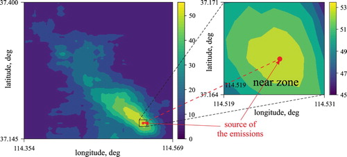
From the formulated conditions (7(7) $\epsilon \sim (P{r}_{D}Re{)}^{-1},$(7) )–(10(10) $T_{obs}\sim \frac{L^2}{P{r}_{D}Re<k>}.$(10) ) it follows that the solution to the problem (1(1) $\begin{array}{rl}& {\epsilon }^2\mathrm{\Delta }u-\epsilon (\mathbf{V}\mathit{(}\mathit{x}\mathit{,}\mathit{y}\mathit{,}\mathit{z}\mathit{)}\cdot \mathrm{grad}\mathit{u})\mathit{+}{\mathit{F}}_{\mathit{N}{\mathit{O}}_{\mathit{2}}}\mathit{(}\mathit{x}\mathit{,}\mathit{y}\mathit{,}\mathit{z}\mathit{)}\mathit{-}<\gamma >\mathit{u}\mathit{=}\mathit{0}\mathit{,}\mathit{(}\mathit{x}\mathit{,}\mathit{y}\mathit{,}\mathit{z}\mathit{)}\in \mathit{D}\mathit{,}\\ & \frac{\mathrm{\partial }u}{\mathrm{\partial }\mathbf{n}}=0,(x,y,z)\in \mathrm{\partial }D.\end{array}$(1) ) can be replaced by its asymptotic approximation (6(6) $\begin{array}{rl}{u}_{\epsilon }(x,y,z)& =\frac{1}{<\gamma >}{F}_{N{O}_2}(x,y,z)-\frac{\epsilon }{<\gamma >}(\mathbf{V}(x,y,z)\cdot \mathrm{grad}{F}_{N{O}_2}(x,y,z))\\ & -(\frac{\epsilon }{<\gamma >\lambda (\theta ,\phi )}\left[\frac{\mathrm{\partial }{F}_{N{O}_2}(r,\theta ,\phi )}{\mathrm{\partial }r}\right]{|}_{r=0}\exp \left(\frac{\lambda (\theta ,\phi )r}{\epsilon }\right)){|}_{\begin{array}{c}r=r(x,y,z)\\ \theta =\theta (x,y,z)\\ \phi =\phi (x,y,z)\end{array}}\\ & +O(\epsilon ).\end{array}$(6) ) for spatial scales (8(8) $l_x,l_y,l_z\sim L\approx P{r}_{D}Re\sqrt{\frac{<k>}{<\gamma >}}.$(8) ) of the order of 1 km, wind speed (9(9) $V\sim \frac{P{r}_{D}Re<k>}{L}.$(9) ) V of the order of $1m/s$ and the time (10(10) $T_{obs}\sim \frac{L^2}{P{r}_{D}Re<k>}.$(10) ) of the continuous and constant operation of the source prior to the moment of receipt experimental data, not less than $30min$. Due to the fact that the picture was taken in the middle of the working day, the condition (10(10) $T_{obs}\sim \frac{L^2}{P{r}_{D}Re<k>}.$(10) ) can be considered fulfilled. The condition (8(8) $l_x,l_y,l_z\sim L\approx P{r}_{D}Re\sqrt{\frac{<k>}{<\gamma >}}.$(8) ) is fulfilled for the near zone with dimensions, for example, 720  m ×720  m($6\times 6$ experimental points). The wind speed required for applying the model (1(1) $\begin{array}{rl}& {\epsilon }^2\mathrm{\Delta }u-\epsilon (\mathbf{V}\mathit{(}\mathit{x}\mathit{,}\mathit{y}\mathit{,}\mathit{z}\mathit{)}\cdot \mathrm{grad}\mathit{u})\mathit{+}{\mathit{F}}_{\mathit{N}{\mathit{O}}_{\mathit{2}}}\mathit{(}\mathit{x}\mathit{,}\mathit{y}\mathit{,}\mathit{z}\mathit{)}\mathit{-}<\gamma >\mathit{u}\mathit{=}\mathit{0}\mathit{,}\mathit{(}\mathit{x}\mathit{,}\mathit{y}\mathit{,}\mathit{z}\mathit{)}\in \mathit{D}\mathit{,}\\ & \frac{\mathrm{\partial }u}{\mathrm{\partial }\mathbf{n}}=0,(x,y,z)\in \mathrm{\partial }D.\end{array}$(1) ) was obtained using the HYSPLIT transport model [29] and became $\mathbf{V}\equiv \mathit{(}{\mathit{V}}_{\mathit{x}}\mathit{,}{\mathit{V}}_{\mathit{y}}\mathit{,}{\mathit{V}}_{\mathit{z}}\mathit{)}\mathit{=}\mathit{(}\mathit{-}\mathit{4.72}\mathit{,}\mathit{7.12}\mathit{,}\mathit{1.02}\mathit{)}{\mathrm{ms}}^{\mathit{-}\mathit{1}}$, which corresponds to the condition (9(9) $V\sim \frac{P{r}_{D}Re<k>}{L}.$(9) ).

To carry out the calculations, a Cartesian coordinate system was used, with a reference point in the lower left corner of the near zone of the source (see the right picture in the Figure 1), whose geographical coordinates are ${114.519}^0$ E, ${37.164}^0$ N, and coordinate axes coinciding with the parallel and the meridian passing through the origin. In this case, the dimensions of the region D take the values $l_x=720$  m, $l_y=720$  m, $l_z=720$  m, and the coordinates of the source: $x_0=290$ m, $y_0=330$ m and $z_0=70$ m. The parameters ϵ, ${\alpha }_{{\mathrm{NO}}_2}$, $\tilde{\gamma }$ and $u_{{\mathrm{O}}_3}(x,y,z)$ for calculating the function (2(2) $F_{{\mathrm{NO}}_2}(x,y,z)={\alpha }_{{\mathrm{NO}}_2}\cdot \tilde{\gamma }\cdot u_{{\mathrm{O}}_3}(x,y,z)\cdot \frac{I}{(2\pi {)}^{3/2}{\sigma }_1^2{\sigma }_2}{\mathrm{e}}^{-(\frac{(x-x_0{)}^2+(y-y_0{)}^2}{2{\sigma }_1^2}+\frac{(z-z_0{)}^2}{2{\sigma }_2^2})},$(2) ) were defined as $\epsilon =0.02$, ${\alpha }_{{\mathrm{NO}}_2}=0.8$, $\tilde{\gamma }=0.001\mathrm{m}{\mathrm{g}}^{-1}{\mathrm{s}}^{-1}{\mathrm{m}}^3$ and $u_{O_3}(x,y,z)=0.02{\mathrm{mgm}}^{-3}$, calculated according to the SILAM model [30].

As the constraints, we use $I_{max}={10}^{28}$ mol(this restriction can be explained by the fact that this corresponds to a thousand-fold excess of the maximum norm), ${{\delta }_1}_{max},{{\delta }_2}_{max}=100$ m(maximum source dimensions) and ${<\gamma >}_{max}={10}^{-2}{\mathrm{s}}^{-1}$ (for the upper limit, we take the laboratory value).

As a result of minimizing the functional (11(11) $G_{\epsilon }[X_{\delta ,\epsilon }]\equiv B[u_{\epsilon }[X_{\delta ,\epsilon }]]=s_{\delta },X_{\delta ,\epsilon }\in \mathrm{\Pi }\subset {{\mathbb{R}}^{\mathbb{+}}}^4.$(11) ) obtained for this data set, the following values of the required parameters were restored: $I=63\cdot {10}^9\cdot {10}^{15}$ molecules, ${\sigma }_1=1.1$ m, ${\sigma }_2=2.3$  m, $<\gamma >=0.001{\mathrm{s}}^{-1}$. Based on these data, the emission power of ${\mathrm{NO}}_2$ was calculated using the formula (2(2) $F_{{\mathrm{NO}}_2}(x,y,z)={\alpha }_{{\mathrm{NO}}_2}\cdot \tilde{\gamma }\cdot u_{{\mathrm{O}}_3}(x,y,z)\cdot \frac{I}{(2\pi {)}^{3/2}{\sigma }_1^2{\sigma }_2}{\mathrm{e}}^{-(\frac{(x-x_0{)}^2+(y-y_0{)}^2}{2{\sigma }_1^2}+\frac{(z-z_0{)}^2}{2{\sigma }_2^2})},$(2) ), which gave a maximum concentration of pollutant in the chimney of about $190{\mathrm{mgm}}^{-3}$, which fully complies with the established standards for permissible emission limits [31].

Remark 1. To find a solution the global optimization package (scipy.optimize) of the Python software was used. The number of algorithm iterations is about ${10}^3$.

Remark 2. Numerical solution of one full direct problem (3(3) $A[X]=u.$(3) ) with the conventional methods on acceptable uniform grids ($N_x\times N_y\times N_z\sim 100\times 100\times 100$, $N_x$, $N_y$, $N_z$ — the number of grid nodes along the axes Ox, Oy, Oz) take about ${10}^3$ seconds. Using asymptotic methods shorten the time needed to solve the direct problem by about 230 times. The calculations were performed under the 64-bit OS Bodhi Linux 5 (v.18.04.1), the processor — Intel Celeron N3060.

Remark 3. Note that the maximum measured (calculated in ${\mathrm{mgm}}^{-3}$ ) pollutant in flue gases is the highest measured or calculated concentration of the pollutant under the worst operating conditions of the boiler, under normal conditions (temperature $0^{o}C$, pressure 101.3 kPa). The maximum emissions of nitrogen oxides are determined by the maximum measured concentrations of these substances. In accordance with [3,3], the limits are set to the maximum emissions. The Directive [3] sets limits on the maximum concentration of a pollutant under normal conditions and air excess factors $\alpha =1.4$ for solid fuel combustion and $\alpha =1.167$ — for gaseous and liquid fuels. These standards are currently in force.

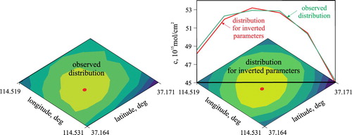
Figure 2 shows the distribution of the integral accumulation of nitrogen dioxide ${\mathrm{NO}}_2$ in the near zone, modelled using the reconstructed parameters, in comparison with the experimentally observed distribution.

Figure 2. The distribution of the height-integral accumulation of nitrogen dioxide ${\mathrm{NO}}_2$ in the near zone obtained using the reconstructed parameters.

4.2. Stability investigation

A numerical study of the stability of the reduced formulation of the inverse problem (11(11) $G_{\epsilon }[X_{\delta ,\epsilon }]\equiv B[u_{\epsilon }[X_{\delta ,\epsilon }]]=s_{\delta },X_{\delta ,\epsilon }\in \mathrm{\Pi }\subset {{\mathbb{R}}^{\mathbb{+}}}^4.$(11) ) was also carried out. The main objective of this study is to show that when solving the inverse problem, we can use the asymptotic approximation (6(6) $\begin{array}{rl}{u}_{\epsilon }(x,y,z)& =\frac{1}{<\gamma >}{F}_{N{O}_2}(x,y,z)-\frac{\epsilon }{<\gamma >}(\mathbf{V}(x,y,z)\cdot \mathrm{grad}{F}_{N{O}_2}(x,y,z))\\ & -(\frac{\epsilon }{<\gamma >\lambda (\theta ,\phi )}\left[\frac{\mathrm{\partial }{F}_{N{O}_2}(r,\theta ,\phi )}{\mathrm{\partial }r}\right]{|}_{r=0}\exp \left(\frac{\lambda (\theta ,\phi )r}{\epsilon }\right)){|}_{\begin{array}{c}r=r(x,y,z)\\ \theta =\theta (x,y,z)\\ \phi =\phi (x,y,z)\end{array}}\\ & +O(\epsilon ).\end{array}$(6) ) of the problem (1(1) $\begin{array}{rl}& {\epsilon }^2\mathrm{\Delta }u-\epsilon (\mathbf{V}\mathit{(}\mathit{x}\mathit{,}\mathit{y}\mathit{,}\mathit{z}\mathit{)}\cdot \mathrm{grad}\mathit{u})\mathit{+}{\mathit{F}}_{\mathit{N}{\mathit{O}}_{\mathit{2}}}\mathit{(}\mathit{x}\mathit{,}\mathit{y}\mathit{,}\mathit{z}\mathit{)}\mathit{-}<\gamma >\mathit{u}\mathit{=}\mathit{0}\mathit{,}\mathit{(}\mathit{x}\mathit{,}\mathit{y}\mathit{,}\mathit{z}\mathit{)}\in \mathit{D}\mathit{,}\\ & \frac{\mathrm{\partial }u}{\mathrm{\partial }\mathbf{n}}=0,(x,y,z)\in \mathrm{\partial }D.\end{array}$(1) ) for a fixed value of the small parameter ϵ and that the stated conditions (7(7) $\epsilon \sim (P{r}_{D}Re{)}^{-1},$(7) )–(10(10) $T_{obs}\sim \frac{L^2}{P{r}_{D}Re<k>}.$(10) ) are true.

For this, calculations were performed for the simulated data $s_{\delta }$ for various error levels δ of input data $s_{\delta }$ and for various values of the small parameter ϵ, which is part of the complete statement of the problem (1(1) $\begin{array}{rl}& {\epsilon }^2\mathrm{\Delta }u-\epsilon (\mathbf{V}\mathit{(}\mathit{x}\mathit{,}\mathit{y}\mathit{,}\mathit{z}\mathit{)}\cdot \mathrm{grad}\mathit{u})\mathit{+}{\mathit{F}}_{\mathit{N}{\mathit{O}}_{\mathit{2}}}\mathit{(}\mathit{x}\mathit{,}\mathit{y}\mathit{,}\mathit{z}\mathit{)}\mathit{-}<\gamma >\mathit{u}\mathit{=}\mathit{0}\mathit{,}\mathit{(}\mathit{x}\mathit{,}\mathit{y}\mathit{,}\mathit{z}\mathit{)}\in \mathit{D}\mathit{,}\\ & \frac{\mathrm{\partial }u}{\mathrm{\partial }\mathbf{n}}=0,(x,y,z)\in \mathrm{\partial }D.\end{array}$(1) ).

Remark. In order to solve problem (1(1) $\begin{array}{rl}& {\epsilon }^2\mathrm{\Delta }u-\epsilon (\mathbf{V}\mathit{(}\mathit{x}\mathit{,}\mathit{y}\mathit{,}\mathit{z}\mathit{)}\cdot \mathrm{grad}\mathit{u})\mathit{+}{\mathit{F}}_{\mathit{N}{\mathit{O}}_{\mathit{2}}}\mathit{(}\mathit{x}\mathit{,}\mathit{y}\mathit{,}\mathit{z}\mathit{)}\mathit{-}<\gamma >\mathit{u}\mathit{=}\mathit{0}\mathit{,}\mathit{(}\mathit{x}\mathit{,}\mathit{y}\mathit{,}\mathit{z}\mathit{)}\in \mathit{D}\mathit{,}\\ & \frac{\mathrm{\partial }u}{\mathrm{\partial }\mathbf{n}}=0,(x,y,z)\in \mathrm{\partial }D.\end{array}$(1) ) we used the Crank–Nicolson method on a fairly dense uniform grids. Subsequent numerical integration of the obtained function u with the aim of simulating $s_{\delta }$ was carried out using the quadrature trapezoid rule.

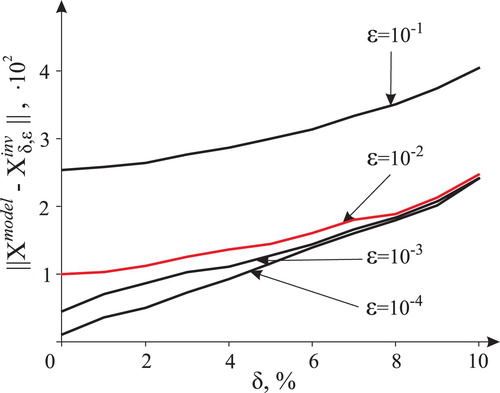
Figure 3 shows a graph of the dependence of the norm of the difference of the model solution $X^{model}$ and the solution $X_{\delta ,\epsilon }^{inv}$ reconstructed using the proposed algorithm from the error δ of the input data for various values of the small parameter ϵ. As can be seen, as the order of smallness of the small parameter ϵ increases, the accuracy of the restoration of the desired set of parameters X increases. Moreover, for typical experimental errors $\sim 5\mathrm{\%}$ of measuring the input data $s_{\delta }$ and the model-specific small parameter value $\sim {10}^{-2}$ the error introduced by the noise δ prevails over the error arising due to the use of the asymptotic solution instead of the exact one.

Figure 3. Dependence of $\Vert X^{model}-X_{\delta ,\epsilon }^{inv}\Vert$ on the noise level δ for different values of the small parameter ϵ.

Remark. The restored parameters ar of very different scales. Thus, the norm with weights was used: $\Vert X\Vert =\sqrt{(w_{1}I{)}^2+(w_2{\sigma }_1{)}^2+(w_2{\sigma }_2{)}^2+(w_3<\gamma >{)}^2},$ where $w_1={10}^{-23}$, $w_2={10}^2$, $w_3={10}^5$. Weights were selected based on a priori information on the characteristic physical scales of the restored parameters ($I\sim {10}^{25}$ mol – characteristic value from regulations, ${\sigma }_{1,2}\sim {10}^2$cm – characteristic pipe dimensions, $<\gamma >\le {10}^{-2}{\mathrm{s}}^{-1}$ – laboratory value).

5. Conclusion

The work demonstrated the possibilities of asymptotic analysis methods for solving the inverse problem of restoring the parameters of the source of industrial emissions of nitrogen oxide NO into the atmosphere. The proposed approach is based on a rigorous asymptotic analysis, which allowed to significantly simplify the procedure for solving the subproblem for three-dimensional singularly perturbed equation of the reaction-diffusion-advection type. A feature of the considered approach is that it allowed us to efficiently solve a real applied problem for a fixed value of a small parameter ϵ. This fact significantly distinguishes this work from most works on asymptotic methods, in which asymptotic methods give only asymptotically exact results for the value of the small parameter $\epsilon \to 0$, which is often not applicable for solving real problems. As prospects for the development of the proposed method, it should be noted 1) the implementation of methods for performing a posteriori estimation of the accuracy of the obtained solution [32–38]; 2) modification of the method in order to develop one of the variations of the direct method [39] (the result of which does not depend on the initial approximation, the choice of which is often extremely important in solving nonlinear problems, and uses only the data of the inverse problem) like a globally convergent methods proposed by M. V. Klibanov [40–43].

Disclosure statement

No potential conflict of interest was reported by the author(s).

Additional information

Funding

The work was supported by RFBR (projects no. 18-01-00865 and 18-29-10080). The statement of the problem and the asymptotic analysis of the direct problem were supported by project 18-29-10080. The development and implementation of numerical algorithms for solving the inverse problem were supported by project 18-01-00865.

References

- United States Environmental Protection Agency. 2019. Available from https://www.epa.gov/criteria-air-pollutants.
- Directive 2008/1/ of the European parliament and of the council of 15 January 2008 concerning integrated pollution prevention and control. 2008.
- Directive 2001/80/ec of the European parliament and of the council of 23 October 2001 on the limitation of emissions of certain pollutants into the air from large combustion plants. 2001.
- Gost 17.2.3.02-78. Nature protection. Atmosphere. Regulations for establishing permissible emissions of noxious pollutants from industrial enterprises. 1978. Available from: https://www.russiangost.com/p-16584-gost-172302-78.aspx.
- Convention on long-range transboundary air pollution. Geneva. 1979.
- Hanna S. A simple method of calculating dispersion from urban area sources. J Air Pollut Control Assoc. 1971;21:774–777.
- Kuenen J, Visschedijk A, Jozwicka M, et al. Tnomacc ii emission inventory; a multi-year (2003-2009) consistent high-resolution european emission inventory for air quality modeling. Atmos Chem Phys. 2014;14:10963–10976.
- Elansky N. Air quality and co emissions in the moscow megacity. Urban Climate. 2014;8:42–56.
- Jericevic A, Kraljevic L, Grisogono B, et al. Parameterization of vertical diffusion and the atmospheric boundary layer height determination in the EMEP model. Atmos Chem Phys. 2010;10:341–364.
- Brusseau M, Pepper I, Gerba C. Environmental and pollution science. 3rd ed. London: Academic Press; 2019.
- Elanskii N, Grechko G, Plotkin M, et al. The ozone and aerosol fine structure experiment: Observing the fine structure of ozone and aerosol distribution in the atmosphere from the salyut 7 orbiter. iii – experimental results. J Geophysical Res. 1991;96(D10):18661–18670.
- Burrowsa J, Webera M, Buchwitza M, et al. The global ozone monitoring experiment (gome): mission concept and first scientific results. J Atmos Sci. 1999;56:151–175.
- Levelt P, Hilsenrath E, Leppelmeier GW, et al. Science objectives of the ozone monitoring instrument. IEEE Trans Geoscience and Remote Sensing. 2006;44(5):1199–1208.
- Valks P, Pinardi G, Richter A, et al. Operational total and tropospheric NO2 column retrieval for gome-2. Atmos Meas Tech. 2011;4:1491–1514.
- Vries J, Voors R, Ording B, et al. TROPOMI on ESAS Sentinel 5p ready for launch and use. Proceedings on SPIE. 2016;9688:86–97.
- Geffen J, Eskes H, Boersma K, et al. TROPOMI ATBD of the total and tropospheric NO2 data products. Royal Netherlands Meteorological Institute Ministry of Infrastructure and Water Management. 2019.
- Boersma K, Eskes H, Richter A, et al. Improving algorithms and uncertainty estimates for satellite NO2 retrievals: results from the quality assurance for the essential climate variables (qa4ecv) project. Atmos Meas Tech. 2018;11:6651–6678.
- Postylyakov O, Borovski A, Makarenkov A. First experiment on retrieval of tropospheric NO2 over polluted areas with 2.4-km spatial resolution basing on satellite spectral measurements. Proceedings on SPIE. 2017;10466:633–640.
- Postylyakov O, Borovski A, Elansky N, et al. Comparison of space high-detailed experimental and model data on tropospheric. Proceedings of SPIE. 2019;11208:587–595.
- Lukyanenko D, Shishlenin M, Volkov V. Solving of the coefficient inverse problems for a nonlinear singularly perturbed reaction-diffusion-advection equation with the final time data. Commun Nonlinear Sci Numer Simul. 2018;54:233–247.
- Lukyanenko D, Shishlenin M, Volkov V. Asymptotic analysis of solving an inverse boundary value problem for a nonlinear singularly perturbed time-periodic reaction-diffusion-advection equation. J Inverse and Ill-Posed Problems. 2019;27(5):745–758.
- Lukyanenko D, Grigorev V, Volkov V, et al. Solving of the coefficient inverse problem for a nonlinear singularly perturbed two-dimensional reaction-diffusion equation with the location of moving front data. Computers and Math Appl. 2019;77(5):1245–1254.
- Davydova M, Nefedov N, Zakharova S. Asymptotically Lyapunov-stable solutions with boundary and internal layers in the stationary reaction-diffusion-advection problems with a small transfer. Lecture Notes Computer Sci. 2019;11386:216–224.
- Samarskii A, Vabishchevich P. Computational heat transfer. Chichester: Wiley; 1995. Mathematical Modelling
- Lavrentiev M. On integral equations of the first kind. Dokl Akad Nauk SSSR. 1959;127(1):31–33.
- Tikhonov N. Regularization of incorrectly posed problems. Dokl Akad Nauk SSSR. 1963;153(1):49–52.
- Vasin V, Ageev A. Ill-posed problems with a priori information. Utrecht: VSP; 1995.
- Resurs-p. 2019. Available from http://russianspacesystems.ru/bussines/dzz/orbitalnaya-gruppirovka-ka-dzz/resurs-p/.
- Hysplit. 2019. Available from https://www.ready.noaa.gov/HYSPLIT.php.
- Silam. 2019. Available from http://silam.fmi.fi/index.html.
- Mitsuru M, Jongkyun L, Ichiro K, et al. Improving emission regulation for coal-fired power plants in asean. 2016. (ERIA Research project report; 2).
- Yagola A, Leonov A, Titarenko V. Data errors and an error estimation for ill-posed problems. Inverse Problems in Eng. 2002;10(2):117–129.
- Dorofeev K, Titarenko V, Yagola A. Algorithms for constructing a posteriori errors of solutions to ill-posed problems. Comput Math and Math Phys. 2003;43(1):10–23.
- Titarenko V, Yagola A. Error estimation for ill-posed problems on piecewise convex functions and sourcewise represented sets. J Inverse and Ill-Posed Prob. 2008;16(6):625–638.
- Yagola A, Korolev Y. Error estimation in ill-posed problems in special cases. 48. 2013, p. 155–164. (Springer Proceedings in Mathematics and Statistics;
- Leonov A. Error estimation in ill-posed problems in special cases. Which of inverse problems can have a priori approximate solution accuracy estimates comparable in order with the data accuracy. Vol. 7, 2014. p. 284–292.
- Leonov A. A posteriori accuracy estimations of solutions to ill-posed inverse problems and extra-optimal regularizing algorithms for their solution. Numer Anal Appl. 2012;5(1):68–83.
- Tikhonov A, Goncharsky A, Stepanov V, et al. Numerical methods for the solution of ill-posed problems. Dordrecht: Kluwer Academic Publishers; 1995.
- Kabanikhin S. Definitions and examples of inverse and ill-posed problems. J Inverse Ill-Posed Prob. 2008;16(4):317–357.
- Beilina L, Klibanov M. Definitions and examples of inverse and ill-posed problems. SIAM J Sci Comput. 2008;31(1):478–509.
- Klibanov M, Fiddy M, Beilina L, et al. Picosecond scale experimental verification of a globally convergent algorithm for a coefficient inverse problem. Inverse Probl. 2010;26(4):045003.
- Klibanov M, Koshev N, Li J, et al. Numerical solution of an ill-posed cauchy problem for a quasilinear parabolic equation using a Carleman weight function. J Inverse Ill-Posed Prob. 2016;24:1–6.
- Klibanov M, Yagola A. Convergent numerical methods for parabolic equations with reversed time via a new Carleman estimate. Inverse Probl. 2019;26(11):115012.