Characterization of electromagnetic parameters through inversion using metaheuristic technique

Abstract

Inverse problems are of importance in many fields of science and engineering. Electromagnetic inversion deals with estimating information contained in electromagnetic measurements. The inversion scheme needs to be designed properly to compensate for Gibbs oscillations effects in the solution, and hence give better validation for the estimated quantities. In this paper an inversion methodology based on simulated annealing is presented that has the ability to extract information about electrical conductivity and dielectric permittivity of a vertically stratified medium using the scattered electric field. Furthermore, Gibbs phenomenon and its oscillation effect on the inversion solution have been studied, and an efficient approach has been developed to render more accurate estimations. Results of implementing the proposed approach and its resolution compared with the original methodology are presented.

KEYWORDS:

• Inversion
• metaheuristic
• oscillation reduction
• simulated annealing

2010 MATHEMATICS SUBJECT CLASSIFICATIONS:

• 45C05
• 45Q05
• 65R15

1. Introduction

During the last century, electromagnetic (EM) methods have been widely used in several applications, i.e. mining industry, ground water exploration, and environmental monitoring, etc. [1,2]. Most of the electromagnetic methods attempt to measure the properties of a medium which are described by its electric permittivity, magnetic permeability, and electric conductivity [3]. In the EM inversion process, one considers the problem of estimating these values based on EM scattering data from various scatterers in the defined domain [4,5].

Inversion of EM data requires a number of repeated solutions with an accurate forward model in an iterative process [6,7]. The computational efficiency of the forward model will, therefore, strongly influence the computational efficiency of the inversion. There are several techniques available for EM forward modelling based on numerical solution of Maxwell’s differential equations, i.e. Finite difference or Finite element methods [8,9]. However, for such conventional numerical methods there are limitations, including numerical dispersion and numerical polarization [10,11], the need to truncate the computational domain, hence, the introduction of unphysical non-reflecting boundaries, the difficulty of representing highly localized sources, the bad accuracy near points where the field is singular [12,13]. In this paper, we developed an approach to overcome some of these limitations and difficulties. Thus, one of the objectives of this paper is developing and analysing an accurate forward modelling method to be used in an optimal setting with inversion modelling.

Inverse scattering problems are in general nonlinear and ill-posed problems [14]. Several approaches deal with the problem as it is, i.e. nonlinear [15,16], while others linearize the problem first, then find a solution for the linear problem [17]. However, the final solution of the linear problem may not be related to the actual solution of the nonlinear one. Another objective of this paper is to develop an inversion methodology, where we have taken the approach of dealing with the inverse nonlinear problem as it is.

In our inversion setting, we present a strategy where the forward solver (or at least part of it) will be used repeatedly for different values of the unknown conductivity and permittivity in a form of a global optimization problem that we then solve using a simulated annealing algorithm. Simulated annealing is a probabilistic technique for approximating the global optimum of a given function [18]. Specifically, it gives an approximate global optimization in a large search space. For problems where finding the precise global optimum is less important than finding an acceptable global optimum in a fixed amount of time, simulated annealing is preferable to alternative methods that may require expensive computations and need much time to reach the final solution.

On the other hand, due to the nature of both the problem, and the proposed forward problem solution, the inverse scheme representation may suffer from oscillations near the discontinuities of the medium parameters. These oscillations are known by Gibbs phenomenon [19,20]. Gibbs phenomenon is relevant to many areas of science and engineering and its effect may extend beyond the discontinuity and influences the function approximation at all points in the physical space and may deteriorate the solution stability [21,22]. For this reason, in this paper, we studied the oscillatory behaviour, i.e. Gibbs oscillations of the inversion solution at the interval boundaries of the used model using the proposed approach. Then to gain more confidence in the physical representation of the forward problem and to decrease the uncertainty in the inverse solution, a developed procedure is introduced to reduce this oscillations effect, and provide more accurate solution.

2. Forward formulation

The solution of the proposed forward problem is to obtain the scattered field reflected from an inhomogeneous vertically stratified layered model. Now consider an infinite unphased electric line source in the y direction acting as a transmitter leading to an electric field in the y direction. We want to compute the field scattered from the inhomogeneity back to the background medium. For a harmonic time dependence of the form $e^{-i\omega t}$, Maxwell’s equations inside the scatterer can be defined as [23] (1) $\begin{array}{rl}\mathrm{\nabla }\times H(x,z)& =(-iw{ϵ}_0{ϵ}_r(x,z)+\sigma (x,z))E(x,z),\end{array}$(1) (2) $\begin{array}{rl}\mathrm{\nabla }\times E(x,z)& =iw{\mu }_0{\mu }_r(x,z)H(x,z),\end{array}$(2) where $E(x,z)$ is the electric field, $H(x,z)$ is the magnetic field, ${ϵ}_r(x,z)$ is the relative permittivity, $\sigma (x,z)$ is the conductivity, and ${\mu }_r(x,z)$ is the relative permeability of the scatterer. In addition, ${ϵ}_0$ is the permittivity of free space, μ₀ is the permeability of free space (taken as the background medium without loss of generality). The operating frequency is given by ω/2π. Meanwhile, in free space, the Maxwell’s equations are given by [24] (3) $\begin{array}{rl}\mathrm{\nabla }\times H(x,z)& =-iw{ϵ}_{0}E(x,z)+J(x,z),\end{array}$(3) (4) $\begin{array}{rl}\mathrm{\nabla }\times E(x,z)& =iw{\mu }_{0}H(x,z)+M(x,z),\end{array}$(4) where $J(x,z)$ is an electric current source and $M(x,z)$ is a magnetic current source, hence, the scatterer presence in free space can be thought of as an electric polarization, $J(x,z)$, and a magnetic polarization,$M(x,z)$ currents given by [25] (5) $\begin{array}{rl}J(x,z)& =(\sigma (x,z)-iw{ϵ}_0({ϵ}_r(x,z)-1))E(x,z),\end{array}$(5) (6) $\begin{array}{rl}M(x,z)& =-iw{\mu }_0({\mu }_r(x,z)-1)H(x,z).\end{array}$(6)

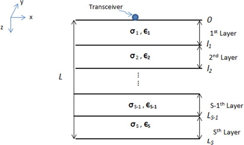
Other approaches can be used as a forward model to solve the problem [26,27]. However, the proposed formulation in this paper offers more generalized forward model that can deal with cases where permittivities and/or conductivities are function(s) of $z$ and/or $x$ direction per layer (i.e.$\sigma \left(x,z\right)\text{and/or}{ϵ}_r\left(x,z\right)\text{; per}\text{layer}$. ). As shown in Figure 1, we will limit the current analysis to a vertically stratified layered medium, i.e. dielectric permittivity ${ϵ}_r$, and electric conductivity σ are inhomogeneous along the z direction only. A further assumption is that µ is everywhere equal to the permeability of the free space μ₀. For the sake of simplicity, we assume a perfect dielectric case, ${\mu }_r(z)$ = 1, hence, $M(x,z)$ = 0. Therefore, for such a y-independent problem and no magnetic currents, the nonvanishing field components are the electric field in the y-direction and the magnetic fields in the x and z directions. The electric field inside the scatterer is given by [28] (7) $\begin{array}{rl}{E}_{ym}(x,z)& =E_y^0(x,z)-\frac{w{\mu }_0}{4}{\int }_0^L{\int }_{-\mathrm{\infty }}^{\mathrm{\infty }}{J}_y\left(\stackrel{`}{x},\stackrel{`}{z}\right)H_0^{(1)}\left(x,z,\stackrel{`}{x},\stackrel{`}{z}\right)d{z}^{\mathrm{\prime }}d{x}^{\mathrm{\prime }},\end{array}$(7) (8) $\begin{array}{rl}{E}_y^0(x,z)& =-\frac{w{\mu }_0}{4}{H}_0^{(1)}(k_0|\rho -{\rho }_s|),\end{array}$(8) (9) $\begin{array}{rl}{H}_0^{(1)}(k_0|\rho -{\rho }_s|)& =\frac{1}{\pi }{\int }_{-\mathrm{\infty }}^{\mathrm{\infty }}\frac{\text{exp}(i{k}_x(x-x^{\mathrm{\prime }})+i{k}_z|z-z^{\mathrm{\prime }}|)}{k_z}d{k}_x,\end{array}$(9) $\begin{array}{rl}{k}_z& =\sqrt{k_0^2-k_x^2}\text{ with img }{k}_z>0,\end{array}$

Figure 1. The general model of a vertically stratified S layers with an overall thickness of L.

where $E_{ym}(x,z)$ is the total field inside the medium, $E_y^0(x,z)$ is the incident electric field, $H_0^{(1)}$(.) is the Hankel function of order zero and first kind, $k_0=w\sqrt{{\mu }_0{ϵ}_0}$ is the free space wave number, and $\rho$ and ${\rho }_s$ are the location of an observation point and source point respectively. $(x,z)$ is the Cartesian coordinate of an observation point, ($x^{\mathrm{\prime }},z^{\mathrm{\prime }}$) is the Cartesian coordinate of the polarization current. The double integral is on the geometry of the scatterer with L standing for the overall thickness of the vertically stratified scatterer with S layers along the z-direction, see Figure 1.

Hence, (10) $\begin{array}{r}{J}_y(x,z)=[\sigma (z)-iw{ϵ}_0({ϵ}_r(z)-1)]E_{ym}(x,z).\end{array}$(10) The line source is located at x_s = z_s = 0. Taking the Fourier transform on x, we obtain for L ≥ z ≥ 0 (11) $\begin{array}{rl}{J}_y(k_x,z)& =Q(z)\left[\frac{i\text{exp}(i{k}_{z}z)}{2k_z}+{\int }_0^L{J}_y(k_x,z^{\mathrm{\prime }})\frac{iexp(i{k}_z|z-z^{\mathrm{\prime }}|)}{2k_z}d{z}^{\mathrm{\prime }}\right],\end{array}$(11) $\begin{array}{rl}\text{and}{J}_y(k_x,z)& =0,L<z<0,\end{array}$which represents an integral equation in z for each k_x with (12) $\begin{array}{r}Q(z)=\{\sigma (z)-iw{ϵ}_0({ϵ}_r(z)-1)\}iw{\mu }_0=k_2^2(z)-k_0^2,\end{array}$(12) where $k_2^2(z)=w^2{\mu }_0{ϵ}_0{ϵ}_r(z)+iw{\mu }_0\sigma (z).$

Now Maxwell’s equations inside the scatterer are rewritten in the form of a volume integral equation on the electric polarization current [29]. Moving forward, we will solve the integral equation eigenvalue problem (13) $\begin{array}{r}{\int }_0^L\frac{i\text{exp}(i{k}_z|z-z^{\mathrm{\prime }}|)}{2k_z}{\psi }_n(k_z,z^{\mathrm{\prime }})d{z}^{\mathrm{\prime }}={\lambda }_n(k_x){\psi }_n(k_x,z),\end{array}$(13) where ${\lambda }_n(k_x)$ stands for the eigenvalue and ${\psi }_n(k_x,z^{\mathrm{\prime }})$ stands for the eigenfunction that satisfy the following equation (14) $\begin{array}{r}\frac{d^2{\psi }_n(k_x,z)}{d{z}^2}+{\alpha }_n^2(k_z){\psi }_n(k_x,z)=0,\end{array}$(14) where ${\alpha }_n^2(k_z)=k_z^2+\frac{1}{{\lambda }_n(k_x)}$, with the boundary conditions (15) $\begin{array}{rl}\frac{d{\psi }_n(k_x,0)}{dz}+i{k}_z{\psi }_n(k_x,0)& =0,\end{array}$(15) (16) $\begin{array}{rl}\frac{d{\psi }_n(k_x,L)}{dz}-i{k}_z{\psi }_n(k_x,L)& =0.\end{array}$(16)

Here we solve the Green’s function problem associated with the differential equation eigenvalue problem, namely, (17) $\begin{array}{rl}\frac{d^{2}g(k_x,z)}{d{z}^2}+\tau g(k_x,z)& =-\delta (z-z^{\mathrm{\prime }}),\end{array}$(17) (18) $\begin{array}{rl}\frac{dg(k_x,0)}{dz}+i{k}_{z}g(k_x,0)& =0,\end{array}$(18) (19) $\begin{array}{rl}\frac{dg(k_x,L)}{dz}-i{k}_{z}g(k_x,L)& =0.\end{array}$(19)

This leads to a complete discrete orthonormal set {${\psi }_n(k_x,z)$}, with each element having its corresponding eigenvalue (${\lambda }_n(k_x)$). Now, we apply the eigenfunctions in the integral equation of $J_y(k_x,z)$ (20) $\begin{array}{rl}{J}_y(k_x,z)& =\sum _n{J}_n(k_x){\psi }_n(k_x,z),\end{array}$(20) (21) $\begin{array}{rl}\frac{i\text{exp}(i{k}_{z}z)}{2k_z}& =\sum _n{\lambda }_n(k_x){\psi }_n(k_x,0){\psi }_n(k_x,z),\end{array}$(21) with {$J_n(k_x)$} as the expansion coefficients of $J_y(k_x,z)$ in terms of the complete orthonormal set {${\psi }_n(k_x,z)$}. Now we make use of the orthonormality of the set {${\psi }_n(k_x,z)$}, [30] namely, (22) $\begin{array}{r}{\int }_0^L{\psi }_m(k_x,z){\psi }_n(k_x,z)dz={\delta }_{mn},\end{array}$(22) to obtain (23) $\begin{array}{rl}{J}_m(k_x)& =\sum _n{\lambda }_n(k_x){\psi }_n(k_x,0)Q_{mn}(k_x)+\sum _n{J}_n(k_x){\lambda }_n(k_x)Q_{mn}(k_x),\end{array}$(23) (24) $\begin{array}{rl}{Q}_{mn}(k_x)& ={\int }_0^L{\psi }_m(k_x,z)Q(z){\psi }_n(k_x,z)dz.\end{array}$(24) This forms a linear system solution of the form: (25) $\begin{array}{r}J(k_x)=(I-M(k_x){)}^{-1}c(k_x),\end{array}$(25) where $M(k_x)=\text{Diag}({\lambda }_n(k_x))Q(k_x)$ and $c(k_x)=\sum _n{\lambda }_n(k_x){\psi }_n(k_x,0)Q_{mn}(k_x),n,m=1,2,\dots N$ and I stands for the unit matrix of size N, where N is the total number of eigenfunctions to be included in the representation. Once we compute the coefficients$\{J_n(k_x)\}$, the scattered electric field's distribution is obtained at the receiver (26) $\begin{array}{r}{E}_{ys}(k_x,0)=i\omega {\mu }_0\sum _n{J}_n(k_x){\lambda }_n(k_x){\psi }_n(k_x,0).\end{array}$(26)

3. Inversion scheme

The target of inversion scheme is to estimate the dielectric permittivity and the electric conductivity of each layer in the model given the scattered electric field at the receiver through an iterative process in order to reduce the misfit between the initial and the actual model. Linear inversion is extensively explained in the literature, often along with general inverse theory [31,32]. Despite its major importance for understanding many aspects of inverse theory, in this paper we regard it as a special case of nonlinear inversion.

In our approach, the forward problem is an integral part of the inverse problem as it is used iteratively in the optimization based scheme. So, here the inversion process which is nonlinear in nature is reformulated in terms of solution of set of linear equations in order to get the current expansion coefficients$J(k_x)$. However, the final inversion equation is still nonlinear in terms of finding the unknown physical parameters of each layer from the current expansion coefficients$J(k_x)$. For this reason the iterative process in the inversion scheme was done in the form of a global optimization problem using the simulated annealing method [33–35]. There is a need to incorporate a priori information about the possible range of physical parameters of each layer in the model. In this paper, optimization of the inversion result is done through an objective function, $\text{OF}$, constructed in the form (27) $\begin{array}{r}\text{OF}=\sum _{m=1}^M|E_m^m-E_c^m{|}^2,\end{array}$(27) where $E_m^m$ is the measured electrical field collected at the mth wavenumber and $E_c^m$ is the electric field computed from a guess of what the model’s layers materials properties and thickness might be. However, for simplicity, we consider that each layer thickness is known, and the analysis here is limited to identify only the 2S material properties of the S layers. Hence, the objective function is 2S-dimensional (28) $\begin{array}{r}\text{OF}(\{{\epsilon }_{rs}\},\{{\sigma }_s\},s=1:S),\end{array}$(28) where $\{{\epsilon }_{rs}\},\{{\sigma }_s\}$ are the relative permittivity and conductivity respectively, of the sth layer.

Several approaches can be used to solve an optimization problem such as Genetic algorithm, and Neural Network, etc. While Genetic algorithm is computationally expensive, and Neural Network requires a huge set of training examples to find an optimum solution, the simulated annealing method has the advantage of being flexible with respect to the evolutions of the problem and easy to implement. The technique of simulated annealing is based on the physical analogy of cooling crystals that, when cooled very slowly, attempt to arrive at its globally minimal potential energy [36]. Simulated annealing interprets slow cooling as a slow decrease in the probability of accepting worse solutions as it explores the solution space. Accepting worse solutions is a fundamental property of the technique because it allows for a more extensive search for the optimal solution through the ability to escape local minima [37].

Here, the simulated annealing algorithm starts with an initial temperature, and generates random estimates for the 2S material properties, driven from the possible range of physical parameters of each layer in the model, and these estimates considered as proposed estimates. The algorithm chooses the distance between the proposed estimates and the current estimates by a probability distribution depending on the current temperature, and the direction of the step is uniformly random.

After that, the algorithm determines whether the proposed estimates are better or worse than the current ones by applying the defined objective function, $\text{OF}$. If the new objective function value is less than the old, the proposed estimates are accepted and become the new current estimates. If the proposed estimates are worse than the current ones, the algorithm can still accept the proposed estimates as the new current estimates, but with a probability based on an acceptance function. (29) $\begin{array}{r}\text{AF}=\frac{1}{1+\text{exp}\left(\frac{{\text{OF}}_{\text{proposed}}-{\text{OF}}_{\text{current}}}{T}\right)},\end{array}$(29) where ${\text{OF}}_{\text{proposed}}$ is the objective function value of the proposed estimates, ${\text{OF}}_{\text{current}}$ is the objective function value of the current estimates and T is the current temperature.

The probability of acceptance is between 0 and 0.5. Thus, AF is then compared with a random number P, generated between [0 0.5]. If $\text{AF}$ > P the uphill change is accepted. Simulated annealing gradually decreases the probability of accepting worse estimates as the algorithm proceeds. This is done according to cooling schedule T(c), whereas temperature decreases, the acceptance probability decreases as well. In this paper, three simulated annealing cooling schedules are designed, implemented and compared for performance (30) $\begin{array}{rl}\text{Exponential}T(c)& ={\alpha }^b{T}_i,\end{array}$(30) (31) $\begin{array}{rl}\text{Fast}T(c)& =\frac{T_i}{b+1},\end{array}$(31) (32) $\begin{array}{rl}\text{Boltzmann}T(c)& =\frac{T_i}{\ln (b+1)},\end{array}$(32) where b = 1, 2, 3 … is the iteration number, $T_i$ is the initial temperature and $\alpha$ is the cooling rate.

Here we use 100°C and 0.95 as values for initial temperature and cooling rate respectively for the three cooling schedules. The Simulated annealing algorithm has an objective to minimize the error between the estimated and calculated value reaching an optimum value of 0%. However, if it fails to do so, we determine stopping criteria of 10,000 iterations, after that, the algorithm outputs the results achieving the nearest value to the optimum.

4. Simulation results

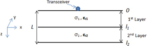
To find the layer’s physical properties, we convert the inverse scattering problem into a global minimization one. The Electromagnetic fields scattered from the inhomogeneous layered model are collected at M wave numbers. In this paper, we limit the problem formulation to find the four physical properties of a two-layer model, given the measured scattered electromagnetic fields at M wavenumbers. The forward model is shown in Figure 2 where both transmitter and receiver are located at the same point just above the top of the model. The thickness of the first layer l₁ is 500 m, and the same for the second layer l₂, giving a total model depth of L = 1000 m.

Figure 2. The proposed model in this paper.

In this paper, we selected seven possible configurations to construct possible layered models from it. Table 1 summarizes the possible permittivity, and conductivity, ranges of these configurations, which is taken from permittivity, and conductivity, ranges of some geological formations [38]. However, it is worth to mention that any physical ranges from other applications of interest can be used as well.

Table 1. Physical properties of the seven configurations along with their spread factor.

Config. no.	Relative permittivity range ${ϵ}_r$	${ϵ}_r$ Spread factor (%)	Conductivity range $\sigma$	$\sigma$ Spread factor (%)
1	4–8	66.66	1 x10^−4–2 × 10^−3	180.95
2	4.8–18.9	118.98	0.001–0.005	133.33
3	4.7–12	87.42	1.25 × 10^−4–0.001	155.55
4	3.9–29.4	153.15	0.01–0.02	66.66
5	2.07–2.14	3.32	0.0013–0.25	197.93
6	7–43	144	0.01–1	196
7	50–105	70.96	0.0002–0.002	163.63

Determination of the uncertainty region of certain linear and nonlinear inverse problems needs a certain mathematical structure that can be embedded in the forward physics [39–41]. In this paper, the solution of the forward problem is found semi-analytically in terms of continuous physical parameters. Thus, there is no direct mathematical formula that relates the scattered electric field distribution obtained at the receiver, with the desired physical parameters to be estimated. However, for the reason of uncertainty analysis, we also identify a $spread$ factor that quantifies the wideness of each physical parameter for each layer around the average. The spread factor for each configuration is defined as (33) $\begin{array}{r}\text{Spread }(\text{\%})=\frac{\text{2}(\text{max}\text{value}-\text{min}\text{value})}{\text{max}\text{value + min}\text{value}}\times \text{100}\text{.}\end{array}$(33)

The spread factor is an indication of the worst possible estimate (i.e. worst error) for each physical parameter based on the a priori knowledge. Table 1 summarizes the spread factor for both relative permittivity and conductivity for each configuration used in this paper. It can be noticed that except for the constant relative permittivity of the 5th case, the spread factor of the relative permittivity and conductivity of the four layers are quite large, which put a challenge on the inversion algorithm. We applied our approach on 10 two-layered case studies presented in Table 2. Also, in this paper we define the term relative percentage error δ as follows (34) $\begin{array}{r}\delta =\frac{\text{True }\text{value}-\text{Estimated }\text{value}}{\text{True}\text{value}}\times 100.\end{array}$(34)

Table 2. Physical properties of the ten case studies used in this paper.

Case no.		Configuration no.	Relative permittivity ${ϵ}_r$	Conductivity $\sigma$
1	1st layer	1	5	0.001
	2nd layer	2	15	0.0013
2	1st layer	4	20	0.0133
	2nd layer	3	10	2 × 10^−4
3	1st layer	3	8	1.4286 × 10^−4
	2nd layer	5	2.10	0.002
4	1st layer	3	11	6.6667 × 10^−4
	2nd layer	1	6	0.0004
5	1st layer	3	9	2.5 × 10^−4
	2nd layer	6	40	0.04
6	1st layer	6	30	0.0333
	2nd layer	1	7	0.0017
7	1st layer	7	100	3.33 × 10^−4
	2nd layer	6	35	0.0167
8	1st layer	7	90	4 × 10^−4
	2nd layer	3	12	1.6667 × 10^−4
9	1st layer	7	80	2.8571 × 10^−4
	2nd layer	1	4	1.11 x 10^−4
10	1st layer	7	70	0.0011
	2nd layer	2	18	0.0014

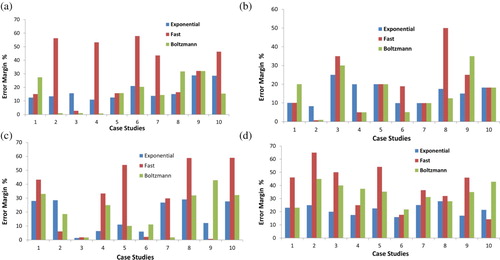
In order to evaluate the performance of different cooling schedules, we calculate the error margin over 100 times for each physical parameter of each layer for each cooling schedule (error margin = $\frac{{\sum }_t\delta }{100},t=1,2,\dots 100$). Results of error margin are presented in Figure 3 where a comparison is made between each cooling schedule per layer. It can be noticed that the error margin resulted from the inversion methodology is quiet low for most of the estimated parameters. Even in cases when $\delta$ is relatively high, the large percentage are far less than the spread factor of the physical parameter. Hence, the a posteriori knowledge is better than the a priori one. Furthermore, the estimated parameter still can be interpreted correctly, as it is within the natural range for each of the investigated layers. So the results are quite acceptable from the error point of view given the non-uniqueness nature of such problems. However, it can be seen that the exponential cooling schedule gives relatively low overall error margins, which does not exceed 30% in the worst case. Meanwhile the fast and Boltzmann cooling schedules give higher error margins, i.e. >30%, in some cases even if they give lower values than the exponential cooling schedule in other cases.

Figure 3. Error margin using exponential, fast, and Boltzmann cooling schedule for the 10 cases of (a) relative permittivity values of the first layer$({ϵ}_{r1})$, (b) conductivity values of the first layer ‘σ₁’, (c) relative permittivity values of the second layer $({ϵ}_{r2})$, (d) conductivity values of the second layer ‘σ₂’.

5. Gibbs oscillations effect

The Gibbs phenomenon can be considered as a drawback in particular when a complete orthonormal set of functions is used to represent a function having discontinuities. One category, namely, intrinsic discontinuities, could be derived from the nature of the physical problems [42]. Another, namely, inherent discontinuities, is created undesirably through the employment of Fourier series [43]. These discontinuities occur at the boundaries between domain parts and lead to oscillations in the represented function [44–46]. In this paper, these oscillations in the polarization current in the forward problem formulation affect the uncertainty of the estimated solution, as the representation of the polarization current in the forward model is not physically accurate.

Several methods have been developed to deal with the reduction of Gibbs oscillations. These methods depend on the nature of the problem as well as the solution approach [47–51]. Figure 4 illustrates an example of the oscillations in the deduced polarization current of the first case study at the first wave number near the boundary interface between the two layers. These oscillations exist in all case studies presented in this paper at all wave numbers. So, in order to reduce the oscillatory behaviour of the polarization current and its effect on the uncertainty of the inversion process, the original inversion scheme has to be updated through updating the forward problem formulation to be more accurate physically. This update in the forward physics will reduce the uncertainty exists in the inverse problem [52], as the forward formulation used iteratively in the presented inversion scheme. In this paper, an alternative representation of the scattered electric field will be used to mitigate the effect of ringing on the inversion solution. Here we will consider the problem as if we have S coupled polarization currents corresponding to S layers. For simplicity, we limit the analysis to a two layered model without loss of generality. Hence we have two coupled polarization currents (35) $\begin{array}{rl}{J}_y^1& =Q_1(z)\left[E_i^{(1)}+{\int }_0^{l_1}G{J}^{(1)}d{z}^{\mathrm{\prime }}+E_{1\leftarrow 2}\right],l_1\ge z\ge 0,\end{array}$(35) (36) $\begin{array}{rl}{J}_y^2& =Q_2(z)\left[E_i^{(2)}+{\int }_{l_1}^{l_2}G{J}^{(2)}d{z}^{\mathrm{\prime }}+E_{2\leftarrow 1}\right],l_2\ge z\ge l_1.\end{array}$(36)

Figure 4. The deduced polarization current of the first case study at the first wave number near the boundary interface between the two layers. (a) the real part, (b) the imaginary part.

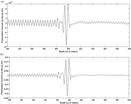
From now on, the superscript (1) and (2) stands for the 1st layer and the 2nd layer respectively. $E_{a\leftarrow b}$ represents the effect of the polarization current from layer b on layer a. $E_i^{(s)}$ stands for the incident electric field. It can be written as (37) $\begin{array}{rl}{E}_i^{(1)}& =\frac{i}{2k_z}exp(i{k}_{z}z),l_1\ge z\ge 0,\end{array}$(37) (38) $\begin{array}{rl}{E}_i^{(2)}& =\frac{i}{2k_z}exp(i{k}_{z}z),l_2\ge z\ge l_1.\end{array}$(38) Here we will solve the two integral equation eigenvalue problems (39) $\begin{array}{rl}{\int }_0^{l_1}G{\psi }_n^{(1)}(k_x,z^{\mathrm{\prime }})d{z}^{\mathrm{\prime }}& ={\lambda }_n^{(1)}(k_x){\psi }_n^{(1)}(k_x,z),\end{array}$(39) (40) $\begin{array}{rl}{\int }_{l_1}^{l_2}G{\psi }_n^{(2)}(k_x,z^{\mathrm{\prime }})d{z}^{\mathrm{\prime }}& ={\lambda }_n^{(2)}(k_x){\psi }_n^{(2)}(k_x,z),\end{array}$(40) $\begin{array}{rl}\text{where}G& =\frac{i}{2k_z}exp(i{k}_z|z-z^{\mathrm{\prime }}|),\end{array}$ (41) $\begin{array}{rl}\text{ and}{Q}_{1,2}& =\{{\sigma }^{(1,2)}-iw{ϵ}_0({{ϵ}_r}^{(1,2)}-1)\}iw{\mu }_0=k_{1,2}^2(z)-k_0^2,\end{array}$(41) (42) $\begin{array}{rl}{k}_{1,2}^2& =w^2{\mu }_0{ϵ}_0{{ϵ}_r}^{(1,2)}+iw{\mu }_0{\sigma }^{(1,2)}.\end{array}$(42)

The eigenfunctions of the second layer ${\psi }_n^{(2)}(k_x,z^{\mathrm{\prime }})$can then be given by (43) $\begin{array}{r}{\psi }_n^{(2)}(k_x,z^{\mathrm{\prime }})=\frac{1}{\sqrt{N_n^2}}[exp(i{\alpha }_n^{(2)}(z-l_1))-\text{exp }(-in\pi )\text{ exp }(i{\alpha }_n^{(2)}(l_2-z))],\end{array}$(43) where ${\alpha }_n^{(2)}(k_x)$ is the solution of the eigenvalue equation (44) $\begin{array}{r}{\alpha }_n^{(2)}=\frac{n\pi }{(l_2-l_1)}-\frac{i}{(l_2-l_1)}\ln \left(\frac{k_z+{\alpha }_n^{(2)}}{k_z-{\alpha }_n^{(2)}}\right),n=1,2,\dots N^{(2)},\end{array}$(44) and $N_n^2$ is a normalization factor given by (45) $\begin{array}{r}{N}_n^2=\frac{i}{{\alpha }_n^{(2)}}[1-exp(2i{\alpha }_n^{(2)}(l_2-l_1))]-2exp(-in\pi )exp(i{\alpha }_n^{(2)}(l_2-l_1))(l_2-l_1).\end{array}$(45)

Now we can rewrite the incident electric field for layer 1 and 2 respectively as (46) $\begin{array}{rl}{E}_i^{(1)}& =\sum {\lambda }_n^{(1)}(k_x){\psi }_n^{(1)}(k_x,0){\psi }_n^{(1)}(k_x,z),\end{array}$(46) (47) $\begin{array}{rl}{E}_i^{(2)}& =\sum {\lambda }_n^{(2)}(k_x){\psi }_n^{(2)}(k_x,l_1){\psi }_n^{(2)}(k_x,z),\end{array}$(47) where ${\lambda }_n^{(1)}(k_x)$and ${\lambda }_n^{(2)}(k_x)$stand for eigenvalues for layer 1 and layer 2 respectively. The effect of the electric field from each layer on the other one can be represented by (48) $\begin{array}{rl}{E}_{1\leftarrow 2}& =2i{k}_z\left[\sum _m{J}_m^{(2)}(k_x){\lambda }_m^{(2)}(k_x){\psi }_m^{(2)}(k_x,l_1)\right]\sum _n{\lambda }_n^{(1)}(k_x){\psi }_n^{(1)}(k_x,0){\psi }_n^{(1)}(k_x,z),\end{array}$(48) (49) $\begin{array}{rl}{E}_{2\leftarrow 1}& =-2i{k}_z\left[\sum _m{J}_m^{(1)}(k_x){\lambda }_m^{(1)}(k_x){\psi }_m^{(1)}(k_x,l_1)\right]\\ & \times \exp (-i{k}_z{l}_1)\sum _n{\lambda }_n^{(2)}(k_x){\psi }_n^{(2)}(k_x,l_1){\psi }_n^{(2)}(k_x,z),\end{array}$(49) where $J_m^{(1)}$and $J_n^{(2)}$are current expansion coefficients of layer 1 and 2 respectively. (50) $\begin{array}{rl}{J}_y^{(1)}(k_x,z)& =\sum _{m=1}^{N^{(1)}}{J}_m^{(1)}(k_x){\psi }_m^{(1)}(k_x,z),\end{array}$(50) (51) $\begin{array}{rl}{J}_y^{(2)}(k_x,z)& =\sum _{n=1}^{N^{(2)}}{J}_n^{(2)}(k_x){\psi }_n^{(2)}(k_x,z).\end{array}$(51)

The Inversion equations can be developed as (52) $\begin{array}{rl}& \sum J_m^{(1)}{\psi }_m^{(1)}(k_x,z)\\ & =Q_1(z)[\sum {\lambda }_m^{(1)}(k_x){\psi }_m^{(1)}(k_x,0){\psi }_m^{(1)}(k_x,z)+\sum J_m^{(1)}{\lambda }_m^{(1)}(k_x){\psi }_m^{(1)}(k_x,z)\\ & +\left[\sum J_n^{(2)}{\lambda }_n^{(2)}{\psi }_n^{(2)}(k_x,l_1)\right]\left[2i{k}_z\sum {\lambda }_m^{(1)}(k_x){\psi }_m^{(1)}(k_x,0){\psi }_m^{(1)}(k_x,z)\right]],\end{array}$(52) (53) $\begin{array}{rl}& \sum J_n^{(2)}{\psi }_n^{(2)}(k_x,z)\\ & =Q_2(z)[\sum {\lambda }_n^{(2)}(k_x){\psi }_n^{(2)}(k_x,l_1){\psi }_n^{(2)}(k_x,z)+\sum J_n^{(2)}{\lambda }_n^{(2)}(k_x){\psi }_n^{(2)}(k_x,z)\\ & +\left[\sum J_m^{(1)}{\lambda }_m^{(1)}{\psi }_m^{(1)}(k_x,l_1)\right]exp(i{k}_z{l}_1)\left[2i{k}_z\sum {\lambda }_n^{(2)}(k_x){\psi }_n^{(2)}(k_x,l_1){\psi }_n^{(2)}(k_x,z)\right]],\end{array}$(53)

After making use of the orthonormality of ${\psi }_m^{(1)}(k_x,z)$for Equation (52), and${\psi }_n^{(2)}(k_x,z)$ for Equation (53), this forms the linear system (54) $\begin{array}{r}{J}_y=(I-D{)}^{-1}c,\end{array}$(54) where $J_y=\left(\begin{array}{c}{J}_y^{(1)}\\ J_y^{(2)}\end{array}\right)$ can be represented in terms of current expansion coefficients as $\left(\begin{array}{c}{J}_1^{(1)}\\ ⋮\\ J_{N^{(1)}}^{(1)}\\ J_1^{(2)}\\ ⋮\\ J_{N^{(2)}}^{(2)}\end{array}\right).$

I stands for the unit matrix of size N, N is the total number of eigenfunctions to be included in the representation, i.e. $N=N^{(1)}+N^{(2)}$.$D$is a symmetric Matrix that is composed of four parts (55) $\begin{array}{rl}D(k_x)& =\left[\begin{array}{cc}{D}_1& C_{2\leftarrow 1}\\ C_{1\leftarrow 2}& D_2\end{array}\right],\end{array}$(55) (56) $\begin{array}{rl}\text{where }{D}_1& =\text{Diag}\left(\frac{1-Q_1{\lambda }_m^{(1)}(k_x)}{Q_1{\lambda }_m^{(1)}(k_x){\psi }_m^{(1)}(k_x,0)}\right),\end{array}$(56) (57) $\begin{array}{rl}{D}_2& =\text{Diag}\left(\frac{1-Q_2{\lambda }_m^{(2)}(k_x)}{Q_2{\lambda }_m^{(2)}(k_x){\psi }_m^{(2)}(k_x,l_1)}\right).\end{array}$(57)

$C_{2\leftarrow 1}$ and $C_{1\leftarrow 2}$ represent matrix coupling of the $J_y^{(1)}$to $J_y^{(2)}$ and $J_y^{(2)}$ to $J_y^{(1)}$respectively. Also (58) $\begin{array}{r}c=\left(\begin{array}{c}c1\\ c2\end{array}\right)=\left(\begin{array}{c}{\lambda }_1^{(1)}{\psi }_1^{(1)}(k_x,0)Q_1\\ ⋮\\ {\lambda }_{N^{(1)}}^{(1)}{\psi }_{N^{(1)}}^{(1)}(k_x,0)Q_1\\ {\lambda }_1^{(2)}{\psi }_1^{(2)}(k_x,l_1)Q_2\\ ⋮\\ {\lambda }_{N^{(2)}}^{(2)}{\psi }_{N^{(2)}}^{(2)}(k_x,l_1)Q_2\end{array}\right).\end{array}$(58)

Once we compute the coefficients $\{J_n^{(1)}(k_x)\}$, and $\{J_m^{(2)}(k_x)\}$, the scattered electric field's distribution is obtained at the receiver, (59) $\begin{array}{rl}{E}_{ys}(k_x,0)& =i\omega {\mu }_0\sum _{m=1}^{N^{(1)}}{J}_m^{(1)}(k_x){\lambda }_m^{(1)}(k_x){\psi }_m^{(1)}(k_x,0)\\ & +\sum _{n=1}^{N^{(2)}}{J}_n^{(2)}(k_x){\lambda }_m^{(2)}(k_x){\psi }_m^{(2)}(k_x,l_1)\text{ ex}{\text{p}}^{-i{k}_z{l}_1}.\end{array}$(59)

The modified forward model results were compared with a frequency domain finite element analysis approach using COMSOL Multiphysics software package. In the finite element analysis, the incident field for the structure of the first case study was a linearly polarized plane wave normalized by $\frac{i}{2k_z}$under a scattering boundary condition. The calculated and the simulated scattered electric field values were compared at 10 wavenumbers ($\text{i}\text{.e}\text{.}{k}_x=0,0.11k_0,0.22k_0,\dots .,0.99k_0)$, and the results are presented at Figure 5. The circles and squares in the figure represent the field computations of the modified forward model approach and the finite element simulation respectively. As shown in the figure, the proposed approach results are very close compared to the finite element analysis solution.

Figure 5. Scattered electric field results at 10 wavenumbers for the first case study using modified forward model (using Equation (59)) and finite element analysis (using COMSOL).

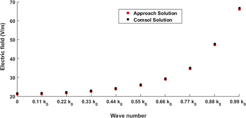
Figure 6 shows an illustration of the efficiency of the modified forward model in reducing the Gibbs oscillations that was presented in Figure 4 for the first case study at the first wavenumber. To realize the impact of the proposed approach in reducing the uncertainty in the inverse solution, we applied this modified approach on the same case studies stated in the previous section, and the results are presented in Figure 7. It can be seen that both the fast and Boltzmann cooling schedules reaches lower error margins than the exponential cooling schedule. However, exponential cooling schedule still gives relatively low overall error margins, that does not exceeds 25% in the worst case. Meanwhile the fast and Boltzmann cooling schedules give higher error margins, i.e. >30%, in some cases even if they give lower values than exponential cooling schedule in other cases.

Figure 6. The deduced polarization current of the first case study at the first wavenumber near the boundary interface between the two layers after applying the oscillation reduction approach. (a) the real part, (b) the imaginary part.

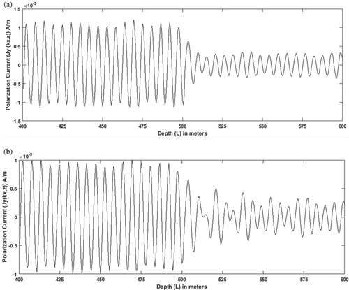
Figure 7. Error margin with oscillation reduction approach using exponential, fast, and Boltzmann cooling schedule for the 10 cases of (a) relative permittivity values of the first layer (${ϵ}_{r1}$), (b) conductivity values of the first layer (σ₁), (c) relative permittivity values of the second layer (${ϵ}_{r2}$), (d) conductivity values of the second layer (σ₂).

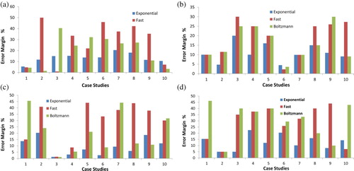
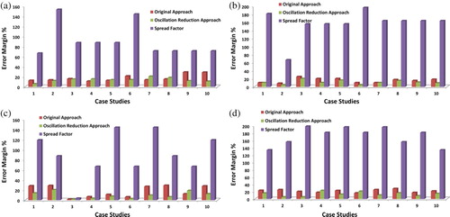
Figure 8 presents a comparison between the error margin results from applying the simulated annealing algorithm with an exponential cooling schedule to the original and oscillation reduction inversion scheme along with the spread factor of each parameter. It is found that the error margin when using the oscillation reduction inversion approach is lower in 76% of the estimated parameters than the original approach. Furthermore, it can be seen that both approaches produce error bounds that are far less than the worst possible estimate for each physical parameter. However, the correct physical representation of the polarization current in the oscillation reduction approach reduces the uncertainty in the inverse solution, as it gives more confidence in the ability of the resultant estimation to construct the observed data using the modified forward model, given the non-uniqueness nature of such problems.

Figure 8. Comparison between the spread factor of each parameter along with the error margin of the original versus oscillation reduction approach using exponential cooling schedule for the 10 cases of (a) relative permittivity values of the first layer (${ϵ}_{r1}$), (b) conductivity values of the first layer (σ₁), (c) relative permittivity values of the second layer (${ϵ}_{r2}$), (d) conductivity values of the second layer (σ₂).

6. Conclusion

In this paper, an approach has been presented to solve the nonlinear inverse scattering problem, where the electric properties (permittivity and conductivity) of a scattering object are estimated from the knowledge of the Electromagnetic source and scattering data. The proposed approach can be used to solve the inverse scattering problem for multilayer medium in different areas of research. The forward model involves a semi-analytical formulation for solving Maxwell's equations, and the inverse scheme is done through the simulated annealing technique. Three cooling schedules have been applied to ten cases and error margins of the estimated parameters have been calculated. It has been found that simulated annealing with exponential cooling schedule is the appropriate inversion technique to be applied on this problem with a worst case error of 30%, and with error bounds far less than the possible worst case estimate error (i.e. spread factor) for each parameter in all case studies.

Furthermore, in order to reduce the uncertainty of the inverse solution, the effect of Gibbs oscillations has been considered, and the forward model has been modified to improve the physical correctness of the forward formulation, and hence give more confidence about the problem solution. After that, the inverse approach has been tested again, and the error results have been compared with the original approach. Updating the forward model physics contributes in that 76 percent of the results show decrease in the error value for the estimated parameters, and again the exponential cooling schedule shows the best results among the investigated ones with error margin less than 25% and with error bounds far less than the possible worst case estimate error (i.e. spread factor) for each parameter in all case studies.

From comparing the spread factor of each physical parameter with the results of the original approach versus the Gibbs oscillations reduction one, it can be seen that both presented inversion schemes gives reasonable estimation of conductivity and permittivity values, in the existence of a large spread factor for each parameter in the studied cases. However, the update of the forward model physics in the Gibbs oscillations reduction inversion scheme results in reducing the uncertainty of the inverse solutions, and hence produce less error margin in 76% of the results of the investigated case studies. Besides, the appropriate physical representation of the polarization current in the forward model leads to more confidence about the resultant estimates of the proposed inversion scheme.

Acknowledgements

The authors would like to thank the anonymous referees for their helpful comments and suggestions to improve the original manuscript.

Disclosure statement

No potential conflict of interest was reported by the author(s).

References

- Li H-J, Lane R-Y. Utilization of multiple polarization data for aerospace target identification. IEEE Trans Antennas Propag. 1995;43(12):1436–1440.
- Pellerin L. Applications of electrical and electromagnetic methods for environmental and geotechnical investigations. Surv Geophys. 2002;23:101–132.
- Stratton JA. Electromagnetic theory. New York: Wiley-IEEE Press; 2007.
- Pierdicca N, Castracane P. Inversion of surface scattering models: comparing criteria and algorithms to estimate bare soil parameters. Proceedings of the IEEE International Geoscience and Remote Sensing Symposium; Ontario, Canada; 2002. p. 1165–1167.
- Yamen F, Yakhno VG, Potthast P. A survey on inverse problems for applied sciences. Math Probl Eng. 2013;2013:1–13.
- Chew WC, Wang YM. Reconstruction of two-dimensional permittivity distribution using the distorted born iterative method. IEEE Trans Med Imaging. 1990;9(2):218–225.
- Dubois A, Belkebir K, Catapano I, et al. Iterative solution of the electromagnetic inverse scattering problem from the transient scattered field. Radio Sci. 2009;44:1–13.
- Taflove A, Hagness SC. Computational electrodynamics: the finite-difference time-domain method. 3rd ed. Boston: Artech House; 2005.
- Jin J. The finite element method in electromagnetics. 2nd ed. New Jersey: John Wiley; 2002.
- Kamel AH. Cost-effective schemes for the numerical simulation of electromagnetic waves. J Electromagn Waves Appl. 1994;8(6):693–710.
- Kamel A, Sguazzero P, Kindelan M. Cost-effective staggered schemes for the numerical simulation of wave propagation. Int J Numer Methods Eng. 1995;38:755–773.
- Caorsi S, Gragnani GL, Pastorino M. Numerical electromagnetic inverse-scattering solutions for two-dimensional infinite dielectric cylinders buried in a Lossy half-space. IEEE Trans Microw Theory Tech. 1993;41(2):352–357.
- Joachimowicz N, Pichot C, Hugonin J-P. Inverse scattering: an iterative numerical method for electromagnetic imaging. IEEE Trans Antennas Propag. 1991;39(12):1742–1753.
- Colton D, Kress R. Using fundamental solutions in inverse scattering. Inverse Probl. 2006;22:R49–R66.
- Colton D, Monk P. A modified dual space method for solving the electromagnetic inverse scattering problem for an infinite cylinder. Inverse Probl. 1994;10(1):87–107.
- Elkattan M. An efficient technique for solving inhomogeneous Electromagnetic inverse scattering problems. J Electromagn Eng Sci. 2020;20(1):64–72.
- Root TO, Stolk CC, de Hoop MV. Linearized inverse scattering based on seismic reverse time migration. Journal de Mathématiques Pures et Appliquées. 2012;98(2):211–238.
- Tan CM. Simulated annealing. London, UK: In-Tech; 2008.
- Libii JN. Gibbs phenomenon and its applications in science and engineering. Proceedings of the American Society for Engineering Education Annual Conference and Exposition; USA; 2005. p. 10.666.1–10.666.12.
- Gelb A, Archibald R. Reducing the Gibbs ringing artifact in MRI scans while maintaining tissue boundary integrity. Proceedings of the IEEE International Symposium on Biomedical Imaging; Washington, DC, USA; 2002. p. 923–926.
- Lim H, Park H. A ringing-artifact reduction method for block-DCT-based image resizing. IEEE Trans Circuits Syst Video Technol. 2011;21(7):879–889.
- Martisek D. Elimination of Gibbs and Nyquist–Shannon phenomena in 3D image reconstruction. 3D Res. 2016;7(16):1–21.
- Collin RE. Foundations for microwave engineering. 2nd ed. New Jersey: John Wiley; 2001.
- Mark AH, Jerry BM. Classical electromagnetic radiation. 3rd ed. New York: Dover; 2012.
- Jin J. Theory and computation of electromagnetic fields. 2nd ed. New Jersey: Wiley–IEEE Press; 2015.
- Nabighian MN. Electromagnetic methods in applied geophysics. Oklahoma: Society of Exploration Geophysicists; 1991.
- Brekhovskikh LM. Waves in layered media. 2nd ed. New York: Academic Press; 1980.
- Felsen L, Marcuvitz N. Radiation and scattering of waves. New Jersey: IEEE Press; 1994.
- Volakis JL, Sertel K. Integral equation methods for electromagnetics. Raleigh (NC): SciTech; 2012.
- Osipov AV, Tretyakov SA. Modern electromagnetics scattering theory with applications. 1st ed. West Sussex: John Wiley; 2017.
- Aster RC, Borchers B, Thurber CH. Parameter estimation and inverse problems. San Diego (CA): Academic Press; 2005.
- Tarantola A. Inverse problem theory and methods for parameter estimation. Philadelphia (PA): SIAM; 2005.
- Hendrix EMT, Tóth BG. Introduction to nonlinear and global optimization. New York: Springer; 2010.
- Dréo J, Pétrowski A, Siarry P, et al. Metaheuristics for hard optimization methods and case studies. 1st ed. Berlin: Springer; 2006.
- Elkattan M, Kamel A. Multiparameter optimization for electromagnetic inversion problem. Adv Electromagn. 2017;6(3):94–97.
- El-Ghazali T. Metaheuristics: from design to implementation. 1st ed. New Jersey: Wiley; 2009.
- Gendreau M, Potvin J-Y. Handbook of metaheuristics. 3rd ed. Switzerland: Springer; 2019.
- Milson J. Field geophysics. 3rd ed. West Sussex: John Wiely; 2003.
- Fernández-Muñiz Z, Hassan K, Fernández-Martínez JL. Data kit inversion and uncertainty analysis. J Appl Geophy. 2019;161:228–238.
- Fernández-Martínez JL, Fernández-Muñiz MZ, Tompkins MJ. On the topography of the cost functional in linear and nonlinear inverse problems. Geophysics. 2012;77(1):W1–W15.
- Fernández-Martínez JL, Fernández-Muñiz MZ, Denys B. The uncertainty analysis in linear and nonlinear regression revisited: application to concrete strength estimation. Inverse Probl Sci Eng. 2019;27(12):1740–1764.
- Li Y-M, Wei D. On the Gibbs phenomenon for linear canonical series expansion. Optik (Stuttg). 2015;126:3605–3612.
- Zhu M H, Li DY. Gibbs phenomenon for fractional Fourier series. IET Signal Proc. 2011;5(8):728–738.
- Zhu H, Ding M, Gao D. Resolution of the Gibbs phenomenon for fractional Fourier series. IEICE Trans Fundam Electron Commun Comput Sci. 2014;E97.A(2):572–586.
- Fikioris G, Andrianesi P. Asymptotic approximations elucidating the Gibbs phenomenon and Fejér averaging. Asymptotic Anal. 2017;102:1–19.
- Jung J-H, Shizgal BD. Generalization of the inverse polynomial reconstruction method in the resolution of the Gibbs phenomenon. J Comput Appl Math. 2004;172:131–151.
- Beckermann B, Matos AC, Wielonsky F. Reduction of the Gibbs phenomenon for smooth functions with jumps by the ϵ-algorithm. J Comput Appl Math. 2008;219:329–349.
- Rim KS, Yun BI. Gibbs phenomenon removal by adding Heaviside functions. Adv Comput Math. 2013;38:683–699.
- De Ridder F, Pintelon R, Schoukens J, et al. Reduction of the Gibbs phenomenon applied on nonharmonic time base distortions. IEEE Trans Instrum Meas. 2005;54(3):1118–1125.
- Kellner E, Dhital B, Kiselev VG, et al. Gibbs-ringing artifact removal based on local subvoxel-shifts. Magn Reson Med. 2016;76:1574–1581.
- Brezinski C. Extrapolation algorithms for filtering series of functions, and treating the Gibbs phenomenon. Numer Algorithms. 2004;36:309–329.
- Scales JA, Snieder R. The anatomy of inverse problems. Geophysics. 2000;65(6):1708–1710.