Inverse problem techniques for multiple crack detection in 2D elastic continua based on extended finite element concepts

Abstract

Two efficient methods are presented to detect multiple cracks in 2D elastic bodies, based on the insights from Extended Finite Element. Adetection mesh is assigned to the cracked body and the responses are measured at the nodes. A finite element model with the same mesh is used to represent the uncracked state of the physical body. In the first method which is called Crack Detection based on Residual Error (CDRE), the residual error norm is calculated based on the uncracked body stiffness matrix and the cracked body responses. The contour of the error norm would show the crack pattern; the method is computationally efficient. In the second method that is coined as Crack Detection based on Stiffness Residual (CDSR), the crack locations are found based on the difference between the stiffness matrix of the cracked body and the uncracked body. The stiffness matrix of the cracked body is found by solving a dynamic inverse problem based on a modified Tikhonov regularization. The efficiency and accuracy of the identification method are enhanced by predicting the crack pattern by the CDRE method. Several examples are presented to show the accuracy and robustness of the methods in the presence of high noise levels.

Keywords:

• Multiple crack detection
• residual error norm
• stiffness identification
• Tikhonov regularization
• X-FEM

2010 Mathematics Subject Classifications:

• 74G75
• 65N21
• 74R10
• 74S05

1. Introduction

Structural health monitoring (SHM) is an important and active field in civil, mechanical and aerospace engineering, and crack detection is an inseparable part of this process [1,2]. In practice, mostly nondestructive methods are used to detect flaws in structures and mechanical components; some examples are, eye detection, dye penetration, ultrasonic and X-ray radiography. Although very useful, these methods are time-consuming, expensive and subjected to human error [3–5].

With the rise in computational power and technology, numerical methods are becoming increasingly popular. Computers can process a large volume of data that are measured by the sensors at different locations of a body, to perform health monitoring. There are several methods to solve the problem of a cracked body subjected to a given loading. Originally proposed by Belytschko et al. [6], the extended finite element method (X-FEM) is one of the best candidates. X-FEM was initially employed in linear elastic fracture mechanics (LEFM) problems, e.g. [7,8], but since then it has been applied to different fields of computational mechanics such as, fatigue [9], ductile fracture [10], contact [11–13], porous media [14,15], fluid-structure interaction [16], etc.; for more details on X-FEM applications consult [17].

Multiple crack detection is intrinsically complicated and expensive. Several X-FEM based methods have been proposed in the literature to solve this problem. Metaheuristic optimization methods, like genetic algorithm (GA) and particle swarm optimization (PSO), have been among the most favourite candidates to be combined with X-FEM. Usually, in these methods, a forward problem is solved iteratively to minimize an error functional. For instance, Rabinovich et al. [18] combined X-FEM with GA to identify the cracks in 2D solids, based on the minimization of the response error defined as the difference between measurements by sensors and the numerical simulation responses at some limited points on the boundary. They used the method to detect single cracks in different orientations. Waisman et al. [19] extended the above method to detect multiple flaws and cracks that were considered to be circular cavities and straight lines. They obtained satisfactory results when there was a sufficient number of sensors, and the flaws were large enough to be detected. They also combined X-FEM with the artificial bee colony algorithm to detect multiple cracks [20]. A noticeable attempt was made by Nanthakumar et al. [21] to detect multiple material interfaces using a regularized level set method. The researchers used X-FEM to iteratively minimize an objective function in order to detect different material discontinuities in piezoelectric structures. Recently, Agathos et al. [22] used X-FEM combined with GA to detect multiple cracks in 3D solids. They used a two-step methodology; first, an estimation of the number of the cracks was found and second, the locations of the cracks were determined by the evolutionary optimization method. Khatir et al. [23] used X-FEM with PSO to detect flaws in plate structures. Other combinations of X-FEM and PSO are found in [24,25] and [26].

Although very appealing, the metaheuristic optimization methods have few drawbacks. First, they need to solve the forward problem hundreds or thousands of times. Second, the computational expenses grow exponentially as the number of state variables increases (curse of dimensionality). Third, there is no guarantee that these methods converge to the exact solution. In fact, these optimization methods may find the local minimum instead of the global one; whereas, it is often the case that complex problems, like multiple crack detection, have several local minimums. An interesting remedy to the high computational costs of these optimization techniques, is to replace the expensive FEM models with simplified ones which correctly capture the physics of the problem while keeping the computational efforts low. In this respect, methods based on machine learning, are a promising solution; for example, Fang and Perera [27] used Response Surface Methodology (RSM) in the damage identification of reinforced concrete structures. Mukhopadhyay et al. [28] employed Random Sampling-High Dimensional Model Representation (RS-HDMR) in combination with multi-objective genetic algorithm optimization technique for damage identification in civil structures. Recently, Mukhopadhyay [29] used Multivariate Adaptive Regression Splines (MARS) in the damage identification of composite bridges. The author, employed Sobol sequences to train the MARS model to improve the convergence rate and to obtain more uniform sampling over the entire design space.

The classic optimization methods, like Lagrange multipliers or gradient descent [30], usually have higher convergence rates, but also have their own drawbacks; first, these methods require the calculation of the objective function derivatives with respect to the state variables. This is both expensive and cumbersome, if not impossible, in case of crack detection problems. Second, these methods need accurate initial guesses; otherwise they may easily converge to a local minimum instead of the global one.

The methods that are presented in this paper are different from the above methods in the sense that they use the stiffness matrix to detect the cracks. The methods are based on the insights from X-FEM. In the first method that is called CDRE, the residual error norm is used as the crack indicator and in the second method which is named CDSR, the stiffness matrix of the cracked body is identified from the measured responses and is then compared with the uncracked body model to detect the locations of the cracks.

System identification has been an active field of research in civil, mechanical and electronic engineering [31]. In this respect, one of the main approaches is grey box identification, in which a governing mathematical model is assumed for the system and the system parameters are found from the responses; for instance, mass, damping and stiffness matrices of a mechanical dynamic system [32] can be determined from different responses like, displacements, stresses, strains, conductivities [33] or temperatures [34]. The identification can be performed in time [35] or frequency domain [36,37] and it can be deterministic or probabilistic; for example, recently, Cao et al. [38] proposed an identification technique, based on sequential first-order second moment reliability method (FOSM) to account for measurement uncertainties.

System identification is, in fact, an inverse problem [39]. One of the main characteristics of the inverse problems is the ill-posedness which manifests itself in high sensitivity to measurement noise. A problem is called well-posed in the sense of Hadamard if the following conditions are met [40]:

1. Existence, it has at least one solution.

2. Uniqueness, the solution is unique.

3. Stability, the outputs are continuously dependent on inputs.

There are several methods to overcome the ill-posedness, amongst which, the regularization techniques are very popular. The main idea of regularization is to include additional constraints to make the problem solvable or stable. There are several regularization methods such as, Tikhonov methods [41], truncated singular value decomposition methods (TSVD) [42], total variation methods [43] and etc. In this respect, Liu et al. [44] proposed a dynamic load identification scheme based on Gegenbauer polynomial expansion theory with Tikhnov regularization for stochastic structures. The authors also proposed a new shpae function method that was combined with interval analysis to determine the dynamic loading on stochastic structures [45]. They employed TSVD regularization technique to solve the inherent ill-posed inverse problem. In this paper, we use a modified version of Tikhonov regularization to identify the stiffness matrix of a cracked body from its displacement responses in the time domain. The objective is to find the closest stiffness matrix to that of the uncracked body. The identified matrix is then compared to the uncracked body stiffness matrix to find the locations of the flaws. The method requires no iterative solution and correctly captures multiple cracks in the presence of high levels of noise.

The structure of the paper is as follows. In section two, the problem of multiple crack detection is stated and insights from X-FEM formulation are explained; the crack detection algorithms are discussed in section three and section four is devoted to numerical examples.

2. Problem statement

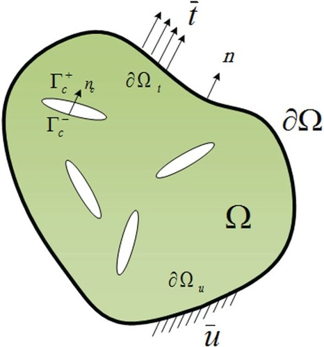
Consider a 2D body Ω with multiple cracks $({\mathrm{\Gamma }}_c{)}_i$, bounded by surface $\mathrm{\partial }\mathrm{\Omega }$ (Figure 1). It is subjected to external time-varying surface tractions $\overline{\mathbf{t}}(t)$ on $\mathrm{\partial }{\mathrm{\Omega }}_t$ and prescribed displacements $\overline{\mathbf{u}}(t)$ on $\mathrm{\partial }{\mathrm{\Omega }}_u$. Considering an isotropic linear elastic material, small deformations and traction free cracks, the equations of motion can be expressed as, (1) $\rho \ddot{\mathbf{u}}=\mathrm{\nabla }.\mathit{\sigma }+\mathbf{b}\mathrm{in}\mathrm{\Omega }$(1) that is subjected to the boundary and initial conditions as (2) $\begin{array}{ll}\mathbf{u}(\mathbf{x},t)=\overline{\mathbf{u}}(\mathbf{x},t)& \mathrm{on}\mathrm{\partial }{\mathrm{\Omega }}_u\\ \mathit{\sigma }.\mathbf{n}=\overline{\mathbf{t}}(\mathbf{x},t)& \mathrm{on}\mathrm{\partial }{\mathrm{\Omega }}_t\\ \mathit{\sigma }.{\mathbf{n}}_c=\mathbf{0}& \mathrm{on}{\mathrm{\Gamma }}_c^{-}\\ \mathit{\sigma }.\mathbf{(}\mathbf{-}{\mathbf{n}}_{\mathbf{c}}\mathbf{)}=\mathbf{0}& \mathrm{on}{\mathrm{\Gamma }}_c^{+}\\ \mathbf{u}(\mathbf{x},0)={\mathbf{u}}_0(\mathbf{x})& \mathrm{in}\mathrm{\Omega }\\ \dot{\mathbf{u}}(\mathbf{x},0)={\dot{\mathbf{u}}}_0(\mathbf{x})& \mathrm{in}\mathrm{\Omega }\end{array}$(2) where ρ is the material density, $\mathbf{u}$, $\dot{\mathbf{u}}$ and $\ddot{\mathbf{u}}$ are the displacement, velocity and acceleration vectors, $\mathit{\sigma }$ is the Cauchy stress tensor, $\mathbf{b}$ is the body force vector and $\mathbf{n}$ is the normal vector to the surface. Note that in this equation the effect of damping is neglected. Here, $(\mathrm{\nabla }.)$ stands for the divergence operator; the derivatives with respect to time are shown with dotted symbols; vectors and tensors are represented with boldface lower and upper case fonts, respectively, and scalars are shown with italic fonts.

Figure 1. Problem statement: 2D body with multiple cracks.

It is worth mentioning that although the assumption of linear elasticity for the body seems restrictive, it can be justified by the fact that most engineering structures are elastic under service loads while they may experience cracking due to fatigue and environmental effects such as corrosion.

The main goal of this paper is to propose methods for multiple cracks detection in the above 2D body. This can be stated as an inverse problem in the following manner: given the geometry, material properties, applied initial and boundary conditions, and the measured responses of the system with some noise, find the locations of the cracks.

2.1. Forward problem: spatial and temporal discretization

The forward problem, that is conjugate to the crack detection inverse problem, can be stated as: given the geometry, cracks, material properties, applied initial and boundary conditions, find the responses of the system.

The solution to this problem is straightforward by conventional numerical methods. The X-FEM which was originally proposed by Belytschko et al. [6] is one of the best candidates. As Figure 2 shows, the main idea of X-FEM is to separate the interfaces from the background mesh so that they can pass through the elements. This removes the remeshing step for moving interface problems like crack propagation. The method is based on the concept of the partition of unity (PUM), proposed by Babuska et al. [46] that allows the inclusion of prior knowledge of the problem by enhancement of the finite element space with enrichment functions. As Equation (3(3) $\begin{array}{rl}\mathbf{u}(\mathbf{x})& =\underset{\mathrm{standard}\mathrm{part}}{\underbrace{\sum _{I\in I_{std}}{\mathbf{N}}_I(\mathbf{x}){\mathbf{u}}_I}}+\underset{\mathrm{Heaviside}\mathrm{enriched}\mathrm{part}}{\underbrace{\sum _{I\in I_H}{\mathbf{N}}_I(\mathbf{x})(H(\mathbf{x})-H({\mathbf{x}}_I)){\mathbf{a}}_I}}\\ & +\underset{\mathrm{Asymptotic}\mathrm{enriched}\mathrm{part}}{\underbrace{\sum _{J=1}^4\sum _{I\in I_{Asy}}{\mathbf{N}}_I(\mathbf{x})({\mathrm{\Phi }}_J(\mathbf{x})-{\mathrm{\Phi }}_J({\mathbf{x}}_I)){\mathbf{b}}_I^J}}\end{array}$(3) ) shows, the displacement field for LEFM problems, has three main parts; the first part is the standard term which is similar to the conventional finite element displacement field and it models the continuous part of the field; the next two parts are the enriched terms which simulate the crack body discontinuity and crack tip singularities, respectively. (3) $\begin{array}{rl}\mathbf{u}(\mathbf{x})& =\underset{\mathrm{standard}\mathrm{part}}{\underbrace{\sum _{I\in I_{std}}{\mathbf{N}}_I(\mathbf{x}){\mathbf{u}}_I}}+\underset{\mathrm{Heaviside}\mathrm{enriched}\mathrm{part}}{\underbrace{\sum _{I\in I_H}{\mathbf{N}}_I(\mathbf{x})(H(\mathbf{x})-H({\mathbf{x}}_I)){\mathbf{a}}_I}}\\ & +\underset{\mathrm{Asymptotic}\mathrm{enriched}\mathrm{part}}{\underbrace{\sum _{J=1}^4\sum _{I\in I_{Asy}}{\mathbf{N}}_I(\mathbf{x})({\mathrm{\Phi }}_J(\mathbf{x})-{\mathrm{\Phi }}_J({\mathbf{x}}_I)){\mathbf{b}}_I^J}}\end{array}$(3) In this equation, ${\mathbf{N}}_I$ is the finite element shape function matrix of node I, H is the Heaviside enrichment function that is used to model the crack body discontinuity and it is defined as (4) $H(\mathbf{x})=\{\begin{array}{ll}-1& \varphi (\mathbf{x})\le 0\\ 1& \varphi (\mathbf{x})>0\end{array}$(4) As Figure 3 illustrates, ϕ is the level-set function which is used to describe the interface geometry and it is usually defined as the signed distance function: (5) $\varphi (\mathbf{x})=\Vert \mathbf{x}-{\mathbf{x}}^{\ast }\Vert \mathrm{sign}({\mathbf{n}}_{{\mathrm{\Gamma }}_d}.(\mathbf{x}-{\mathbf{x}}^{\ast }))$(5) where ${\mathbf{x}}^{\ast }$ is the closest projection of a point $\mathbf{x}$ on the interface and ${\mathbf{n}}_{{\mathrm{\Gamma }}_d}$ is the normal vector to the interface at ${\mathbf{x}}^{\ast }$.

Figure 2. X-FEM enrichment methodology for crack problems [47].

Figure 3. Signed distance function as the level set function which describes the interface. The interface divides an arbitrary domain Ω into two sub-domains ${\mathrm{\Omega }}_A$ with $\varphi (\mathbf{x})>0$ and ${\mathrm{\Omega }}_B$ with $\varphi (\mathbf{x})\le 0$ and the interface is denoted by ${\mathrm{\Gamma }}_d$ which is the zero level set of the signed distance function [17].

In Equation (3(3) $\begin{array}{rl}\mathbf{u}(\mathbf{x})& =\underset{\mathrm{standard}\mathrm{part}}{\underbrace{\sum _{I\in I_{std}}{\mathbf{N}}_I(\mathbf{x}){\mathbf{u}}_I}}+\underset{\mathrm{Heaviside}\mathrm{enriched}\mathrm{part}}{\underbrace{\sum _{I\in I_H}{\mathbf{N}}_I(\mathbf{x})(H(\mathbf{x})-H({\mathbf{x}}_I)){\mathbf{a}}_I}}\\ & +\underset{\mathrm{Asymptotic}\mathrm{enriched}\mathrm{part}}{\underbrace{\sum _{J=1}^4\sum _{I\in I_{Asy}}{\mathbf{N}}_I(\mathbf{x})({\mathrm{\Phi }}_J(\mathbf{x})-{\mathrm{\Phi }}_J({\mathbf{x}}_I)){\mathbf{b}}_I^J}}\end{array}$(3) ), ${\mathrm{\Phi }}_J$s are the four asymptotic enrichment functions which are costume tailored to simulate the crack tip displacement fields, based on analytical LEFM solutions: (6) $\begin{array}{rl}\{{\mathrm{\Phi }}_J\}& =\{\sqrt{r}\sin \left(\frac{\theta }{2}\right),\sqrt{r}\cos \left(\frac{\theta }{2}\right),\sqrt{r}\sin \left(\frac{\theta }{2}\right)\sin (\theta ),\\ & \sqrt{r}\cos \left(\frac{\theta }{2}\right)\sin (\theta )\}\end{array}$(6) where r and θ are the polar coordinates with respect to the corresponding crack tip. In addition, $I_{std}$, $I_H$, and $I_{Asy}$ are the sets of standard, enriched with Heaviside and enriched with asymptotic functions nodes, respectively. ${\mathbf{u}}_I$, ${\mathbf{a}}_I$ and ${\mathbf{b}}_I$ are the corresponding nodal degrees of freedom (dof) vectors. As Figure 2 indicates, the Heaviside enrichment is applied to the nodes of the elements which are cut by the crack body (shown with solid color); the Asymptotic enrichment is applied to the nodes of the elements which are located around the crack tip (shown with upward diagonal hatch), and all other elements are standard and contain no enrichment. Substituting the above displacement field in the weak form of the equation of motion (1(1) $\rho \ddot{\mathbf{u}}=\mathrm{\nabla }.\mathit{\sigma }+\mathbf{b}\mathrm{in}\mathrm{\Omega }$(1) ) results in the following discretized form. (7) $\mathbf{M}\ddot{\mathbf{u}}+\mathbf{K}\mathbf{u}={\mathbf{f}}_{ext}$(7) where (8) $\mathbf{K}={\int }_{\mathrm{\Omega }}{\mathbf{B}}^T\mathbf{D}\mathbf{B}dV$(8) and (9) $\mathbf{M}={\int }_{\mathrm{\Omega }}\rho {\mathbf{N}}^T\mathbf{N}dV$(9) here, ${\mathbf{f}}_{ext}$ is external force vector, and $\mathbf{M}$, $\mathbf{K}$, $\mathbf{B}$, $\mathbf{N}$, and $\mathbf{D}$ are the mass, stiffness, displacement gradient, shape functions, and elastic material properties matrices, respectively. By solving the above system of equations, the unknown standard and enriched degrees of freedom are obtained which can be used to calculate the displacement, strain and stress fields of the domain. For more details on X-FEM formulation and related issues such as blending elements (Figure 2, shown with downward diagonal hatch), consult [17]. Equation (7(7) $\mathbf{M}\ddot{\mathbf{u}}+\mathbf{K}\mathbf{u}={\mathbf{f}}_{ext}$(7) ) needs to be discretized in time; employing the Newmark's direct integration approach, the displacement and velocity fields can be expressed as, (10) $\begin{array}{rl}& {\mathbf{u}}_t={\mathbf{u}}_{t-\mathrm{\Delta }t}+{\dot{\mathbf{u}}}_{t-\mathrm{\Delta }t}\mathrm{\Delta }t+{\ddot{\mathbf{u}}}_{t-\mathrm{\Delta }t}\mathrm{\Delta }{t}^2({\displaystyle \frac{1}{2}}-\beta )+{\ddot{\mathbf{u}}}_t\mathrm{\Delta }{t}^2\beta \end{array}$(10) (11) $\begin{array}{rl}& {\dot{\mathbf{u}}}_t={\dot{\mathbf{u}}}_{t-\mathrm{\Delta }t}+{\ddot{\mathbf{u}}}_{t-\mathrm{\Delta }t}\mathrm{\Delta }t(1-\gamma )+{\ddot{\mathbf{u}}}_t\mathrm{\Delta }t\gamma \end{array}$(11) where $\mathrm{\Delta }t$ is the time step and, β and γ are the two constants of the Newmark's method. For $\gamma \ge 0.5$ and $\beta \ge 0.25$, the method is unconditionally stable and of second-order accuracy for linear elastic problems.

2.2. Insights from X-FEM formulation

One of the key concepts in our crack detection approach is that flaws and cracks reduce the stiffness of the body in certain dofs; this can be shown clearly by the X-FEM formulation. For this purpose, we rewrite Equation (7(7) $\mathbf{M}\ddot{\mathbf{u}}+\mathbf{K}\mathbf{u}={\mathbf{f}}_{ext}$(7) ) in a compact form as, (12) $\mathbf{K}\mathbf{u}=\tilde{\mathbf{f}}$(12) where $\tilde{\mathbf{f}}={\mathbf{f}}_{ext}-\mathbf{M}\ddot{\mathbf{u}}$ is the equivalent dynamic force vector. If we categorize the dofs into standard and enriched sets, Equation (12(12) $\mathbf{K}\mathbf{u}=\tilde{\mathbf{f}}$(12) ) can be rewritten as, (13) $\left[\begin{array}{cc}{\mathbf{K}}_{ss}& {\mathbf{K}}_{se}\\ {\mathbf{K}}_{es}& {\mathbf{K}}_{ee}\end{array}\right]\left[\begin{array}{c}{\mathbf{u}}_s\\ {\mathbf{u}}_e\end{array}\right]=\left[\begin{array}{c}{\tilde{\mathbf{f}}}_s\\ {\tilde{\mathbf{f}}}_e\end{array}\right]$(13) where the subscripts s and e stand for standard and enriched parts, respectively. Using the concept of static condensation, the above equation can be written as, (14) $({\mathbf{K}}_{ss}-{\mathbf{K}}_{se}{\mathbf{K}}_{ee}^{-1}{\mathbf{K}}_{es}){\mathbf{u}}_s={\tilde{\mathbf{f}}}_s-{\mathbf{K}}_{se}{\mathbf{K}}_{ee}^{-1}{\tilde{\mathbf{f}}}_e$(14) In this equation, ${\mathbf{K}}_{ss}$ is equal to the uncracked body stiffness matrix; hence, we define (15) ${\mathbf{K}}_{unc}={\mathbf{K}}_{ss}$(15) and (16) ${\mathbf{K}}_c={\mathbf{K}}_{ss}-{\mathbf{K}}_{se}{\mathbf{K}}_{ee}^{-1}{\mathbf{K}}_{es}$(16) where ${\mathbf{K}}_{unc}$ and ${\mathbf{K}}_c$ are the stiffness matrices of the finite element mesh of the body, excluding and including the effects of the cracks, respectively.

Two important insights can be inferred from the above equations. First, if we rewrite Equation (14(14) $({\mathbf{K}}_{ss}-{\mathbf{K}}_{se}{\mathbf{K}}_{ee}^{-1}{\mathbf{K}}_{es}){\mathbf{u}}_s={\tilde{\mathbf{f}}}_s-{\mathbf{K}}_{se}{\mathbf{K}}_{ee}^{-1}{\tilde{\mathbf{f}}}_e$(14) ) as (17) ${\mathbf{K}}_{unc}{\mathbf{u}}_s-{\tilde{\mathbf{f}}}_s={\mathbf{K}}_{se}{\mathbf{K}}_{ee}^{-1}{\mathbf{K}}_{es}{\mathbf{u}}_s-{\mathbf{K}}_{se}{\mathbf{K}}_{ee}^{-1}{\tilde{\mathbf{f}}}_e$(17) the LHS of the equation states that if the uncracked body stiffness matrix ${\mathbf{K}}_{unc}$ is multiplied by the displacement response of the cracked body ${\mathbf{u}}_s$ and it is subtracted by the force vector ${\tilde{\mathbf{f}}}_s$, the result is kind of a residual error vector which is related to the existence of cracks and flaws (RHS). Note that the RHS is zero in case of no cracks. Thus, if we define the residual error norm $er{r}_i$ for the ith dof as (18) $er{r}_i=\Vert ({\mathbf{K}}_{unc}{\mathbf{u}}_s-{\tilde{\mathbf{f}}}_s{)}_i\Vert \mathrm{for}\mathrm{i}=1,\dots ,\mathrm{n}$(18) where $\Vert .\Vert$ is the norm-2 operator of a vector, the value of $er{r}_i$ can be used as an indicator for the existence of cracks, close to that degree of freedom; n is also the number of dofs in the uncracked body model.

Second, the LHS of Equation (14(14) $({\mathbf{K}}_{ss}-{\mathbf{K}}_{se}{\mathbf{K}}_{ee}^{-1}{\mathbf{K}}_{es}){\mathbf{u}}_s={\tilde{\mathbf{f}}}_s-{\mathbf{K}}_{se}{\mathbf{K}}_{ee}^{-1}{\tilde{\mathbf{f}}}_e$(14) ) shows that the enriched stiffness term ${\mathbf{K}}_{se}{\mathbf{K}}_{ee}^{-1}{\mathbf{K}}_{es}$ is responsible for the stiffness reduction of the standard dofs due to the cracks. In fact, since ${\mathbf{K}}_{ss}$ and ${\mathbf{K}}_{se}{\mathbf{K}}_{ee}^{-1}{\mathbf{K}}_{es}$ are both positive definite and thus have positive diagonal components, the diagonal components of ${\mathbf{K}}_{unc}$ are greater than ${\mathbf{K}}_c$. Hence, if the diagonal components of ${\mathbf{K}}_{unc}$ are subtracted by ${\mathbf{K}}_c$, the dofs that have large residual values determine the locations of the cracks.

These two insights make the foundations of our crack detection algorithms.

3. Crack detection algorithms

Consider a 2D body Ω with multiple cracks (Figure 4(a)). In the proposed detection algorithms, first a mesh grid is assigned to the body which can be assumed as a transparent layer over the domain; the responses are measured at the nodes of this mesh grid. For this purpose, accelerometers or displacement transducers must be placed at the grid nodes and the applied loading must also be logged. It is noted that for a high-resolution crack detection, the grid mesh must be fine; thus the number of required sensors might be unpractical. One promising remedy for this issue is to use video motion capturing and image processing techniques alternatively [48,49]; these methods can provide the full displacement, velocity and acceleration fields of the cracked body with a high accuracy and thus increase the detection resolution to the desired level. Another important issue in the detection process is that the measured data are raw and noisy and thus need preprocessing. De-noising, filtering, and other techniques must be applied to produce higher-quality input data.

Figure 4. Crack identification algorithm: (a) a mesh grid is assigned to the cracked body Ω, and the responses are measured at the grid nodes. (b) a finite element model is constructed with the same geometry, mesh grid, loading, and boundary conditions but without the cracks (uncracked body $\tilde{\mathrm{\Omega }}$).

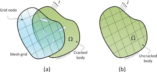
In the next step, a finite element model, which is called the uncracked body $\tilde{\mathrm{\Omega }}$, is constructed from the original cracked body. As Figure 4(b) shows, the model has the same geometry, mesh grid, material properties, loading and boundary conditions as that of the cracked body but it does not contain the cracks. Based on the above framework, two multiple crack detection methods are proposed, which are discussed in the following sections.

3.1. Crack detection based on residual error (CDRE)

The first method, which is called CDRE in short, is simple but very efficient. As it was discussed in Section 2.2, the main idea of the method is to calculate the residual error norm defined as, (19) $er{r}_i=\Vert ({\mathbf{K}}_{unc}\mathbf{u}-\tilde{\mathbf{f}}{)}_i\Vert \mathrm{for}i=1,\dots ,n$(19) ${\mathbf{K}}_{unc}$ is found from the finite element model of the uncracked body (Figure 4(b)). $\mathbf{u}$ and $\tilde{\mathbf{f}}$ are the displacement and dynamic force matrices of the cracked body, respectively; these values are measured at corresponding dofs of the grid nodes in m time steps; hence, they are $n\times m$ matrices.

The residual vector $({\mathbf{K}}_{unc}\mathbf{u}-\tilde{\mathbf{f}}{)}_i$ has m components for the ith dof. A large value of residual error norm $er{r}_i$ indicates that the stiffness matrix ${\mathbf{K}}_{unc}$ can not represent the true system properties at the ith dof. Thus, it suggests the existence of a crack or flaw in the vicinity of the dof. A contour of the residual error norm values in the body shows the probable locations of the cracks.

The method is very efficient in the sense that it only involves a few matrix manipulations; no iteration or solution of a system of equations is thus required.

3.2. Crack detection based on stiffness reduction (CDSR)

The second proposed method, that is called CDSR in short, has two stages: (1) finding an approximation for the stiffness matrix of the cracked body ${\mathbf{K}}_c$, (2) constructing the uncracked body model and comparing its stiffness matrix ${\mathbf{K}}_{unc}$ with ${\mathbf{K}}_c$ to find the locations of the cracks.

Finding the stiffness matrix of the cracked body from the measured responses is an inverse problem which can be expressed as (20) ${\mathbf{K}}_c\mathbf{u}=\tilde{\mathbf{f}}$(20) In this equation, the components of ${\mathbf{K}}_c$ are the unknowns; thus, for a problem with n dofs, there are $n^2$ unknowns. If the symmetry of the stiffness matrix is considered, the number is reduced to $n(n+1)/2$. Also, if the responses are available at m time steps, there would be $m\times n$ equations. Since, usually, the number of equations and unknowns differ, Equation (20(20) ${\mathbf{K}}_c\mathbf{u}=\tilde{\mathbf{f}}$(20) ) can be solved in a least-square manner that is mathematically expressed as the below minimization problem, (21) $\underset{{\mathbf{K}}_c\in {\mathbb{R}}^n\times {\mathbb{R}}^n}{min}\Vert {\mathbf{K}}_c\mathbf{u}-\tilde{\mathbf{f}}{\Vert }^2$(21) A more suitable format of Equation (21(21) $\underset{{\mathbf{K}}_c\in {\mathbb{R}}^n\times {\mathbb{R}}^n}{min}\Vert {\mathbf{K}}_c\mathbf{u}-\tilde{\mathbf{f}}{\Vert }^2$(21) ) is obtained, if the stiffness matrix is converted to a vector of unknowns ${\tilde{\mathbf{k}}}_c$, and the displacement vector is changed into a coefficient matrix $\mathbf{U}$. That is (22) $\underset{{\tilde{\mathbf{k}}}_c\in {\mathbb{R}}^{n^2}}{min}\Vert \mathbf{U}{\tilde{\mathbf{k}}}_c-\tilde{\mathbf{f}}{\Vert }^2$(22) where (23) ${\tilde{\mathbf{k}}}_c={\left[\begin{array}{ccccccccc}{K}_{11}& K_{12}& \cdots & K_{1n}& \cdots & K_{n1}& K_{n2}& \cdots & K_{nn}\end{array}\right]}^T$(23) and, (24) ${\mathbf{U}}_{m\times n,n^2}=\left[\begin{array}{ccccccccccc}{u}_1^1& u_2^1& \cdots & u_n^1& 0& 0& \cdots & 0& 0& \cdots & 0\\ & & & & & \ddots \\ 0& 0& \cdots & 0& 0& 0& \cdots & u_1^1& u_2^1& \cdots & u_n^1\\ & & & & & \ddots \\ u_1^m& u_2^m& \cdots & u_n^m& 0& 0& \cdots & 0& 0& \cdots & 0\\ & & & & & \ddots \\ 0& 0& \cdots & 0& 0& 0& \cdots & u_1^m& u_2^m& \cdots & u_n^m\end{array}\right]$(24) where $u_i^j$ is the displacement component of the ith dof at the jth time step.

The problem of finding the stiffness matrix of a solid body from a finite number of measured responses is inherently ill-posed. Thus, it has all the problems relating to the existence, uniqueness, and stability of the solution. Tikhonov regularization is one of the best classic methods which is very efficient in large problems [40]. In its original form, the method can be expressed as (25) ${\tilde{\mathbf{k}}}_c^{\alpha }=\underset{{\tilde{\mathbf{k}}}_c\in {\mathbb{R}}^{n^2}}{\arg min\{}\Vert \mathbf{U}{\tilde{\mathbf{k}}}_c-\tilde{\mathbf{f}}{\Vert }^2+\alpha \Vert {\tilde{\mathbf{k}}}_c{\Vert }^2\}$(25) where α is a penalty like regularization parameter. For linear problems, this formulation results in a unique solution that can be obtained by solving the equivalent least-square problem. (26) ${\tilde{\mathbf{k}}}_c^{\alpha }=({\mathbf{U}}^T\mathbf{U}+\alpha \mathbf{I}{)}^{-1}{\mathbf{U}}^T\tilde{\mathbf{f}}$(26) where $\mathbf{I}$ is the identity matrix. The problem with the above formulation is that the penalty term $\alpha \Vert {\tilde{\mathbf{k}}}_c{\Vert }^2$, has no physical meaning; as the α parameter increases, the penalty term becomes more dominant; this reduces the absolute values of the stiffness vector ${\tilde{\mathbf{k}}}_c$ components, which can be unrealistic. In fact, α balances the importance of solution discrepancy error versus regularization.

We propose a novel idea to solve the mentioned issue. It is known that the cracked body stiffness is different from the uncracked body; but since the number of cracks is finite, the difference is only significant at few dofs; in other words, the stiffness matrix components are almost identical in both cases, except for few components. We use this fact as a prior knowledge and enforce the solution vector ${\tilde{\mathbf{k}}}_c$ to be as similar as possible to the uncracked stiffness ${\tilde{\mathbf{k}}}_{unc}$. This can be expressed mathematically as, (27) ${\tilde{\mathbf{k}}}_c^{\alpha }=\underset{{\tilde{\mathbf{k}}}_c\in {\mathbb{R}}^{n^2}}{\arg min\{}\Vert \mathbf{U}{\tilde{\mathbf{k}}}_c-\tilde{\mathbf{f}}{\Vert }^2+\alpha \Vert {\tilde{\mathbf{k}}}_c-{\tilde{\mathbf{k}}}_{unc}{\Vert }^2\}$(27) thus, the solution takes the form, (28) ${\tilde{\mathbf{k}}}_c^{\alpha }=({\mathbf{U}}^T\mathbf{U}+\alpha \mathbf{I}{)}^{-1}[{\mathbf{U}}^T\tilde{\mathbf{f}}+\alpha {\tilde{\mathbf{k}}}_{unc}]$(28) This system of equations can be effectively solved with iterative methods such as preconditioned conjugate gradient (PCG). The computational cost of the solution method can be decreased dramatically, if we assume that the sparsity structure of the solution vector ${\tilde{\mathbf{k}}}_c$ is the same as ${\tilde{\mathbf{k}}}_{unc}$. The uncracked stiffness matrix ${\mathbf{K}}_{unc}$ is sparse; thus, approximately $90\mathrm{\%}$ of its components are zero. If we assume the same sparsity structure for ${\mathbf{K}}_c$, the number of unknowns drops to almost $10\mathrm{\%}$ of the original value. Besides, the assumption reduces the ill-conditioningof the problem significantly. Note that the above statement is not perfectly consistent with the Equation (14(14) $({\mathbf{K}}_{ss}-{\mathbf{K}}_{se}{\mathbf{K}}_{ee}^{-1}{\mathbf{K}}_{es}){\mathbf{u}}_s={\tilde{\mathbf{f}}}_s-{\mathbf{K}}_{se}{\mathbf{K}}_{ee}^{-1}{\tilde{\mathbf{f}}}_e$(14) ). However, the gain from the computational efficiency is so prominent that we may neglect the induced inaccuracy.

The identification method is enhanced significantly if different α parameters are used for different dofs. In fact, as it was stated before, ${\mathbf{K}}_{unc}$ and ${\mathbf{K}}_c$ are completely identical, except at a few dofs in the vicinity of cracks. However, if a single α parameter is used, the matrices are enforced to be as similar to each other as possible, in all dofs. Numerical observations showed that this may result in some artefacts in the solution. It is needed to release the similarity constraints at the dofs which are close to the cracks. This is somehow a contradiction; since the location of the cracks must be known beforehand to reduce the penalty factor α for the corresponding dofs. We use the CDRE method, proposed in the previous section, to tackle this issue.

Consider Equation (19(19) $er{r}_i=\Vert ({\mathbf{K}}_{unc}\mathbf{u}-\tilde{\mathbf{f}}{)}_i\Vert \mathrm{for}i=1,\dots ,n$(19) ), the maximum residual error norm $er{r}_{max}$ is defined as, (29) $er{r}_{max}=\underset{i=1,\dots ,n}{max}er{r}_i$(29) The alpha parameter must be high for dofs with low err and vice versa; thus, we define (30) ${\alpha }_i={\displaystyle \frac{{\alpha }_0}{1+{\beta }_0.er{r}_i/er{r}_{max}}}$(30) where ${\alpha }_i$ is the regularization parameter for dof i, ${\alpha }_0$ is the baseline α parameter that is adjusted by the denominator for the dofs with high residual error norms and ${\beta }_0$ is a constant that is used for tuning the denominator.

The final step in the identification process is to compare the stiffness matrix of the cracked body ${\mathbf{K}}_c$ with the uncracked body model ${\mathbf{K}}_{unc}$. To this end, a stiffness reduction vector $\mathbf{d}$ with size  n is constructed from the difference of the diagonal components of the two matrices, as (31) $\mathbf{d}=diag({\mathbf{K}}_{unc}-{\mathbf{K}}_c)$(31) where $diag(.)$ operator returns the main diagonal of the corresponding matrix. Nonzero components of $\mathbf{d}$ represent the changed dofs which are related to cracks and flaws. A simple mapping connects the damage index to the corresponding nodes. The nodal value of the damage is calculated as the square root of the sum of the squares of x and y dofs. The contour of the $\mathbf{d}$ field gives the approximate locations of the cracks.

The identification problems are subject to noise which is always random in nature. In order to investigate the robustness of the proposed methods and to avoid the inverse crime [40], random noise is introduced into the measured responses of the synthetic numerical examples, as following: (32) $\begin{array}{rl}& {\hat{u}}_i=u_i(1+amp.\mathrm{{\rm Y}})\\ & {\hat{\ddot{u}}}_i={\ddot{u}}_i(1+amp.\mathrm{{\rm Y}})\end{array}$(32) where ${\hat{u}}_i$ and ${\ddot{u}}_i$ are noise-contaminated components of the displacement and acceleration vectors of the ‘cracked body’ and $u_i$ and ${\ddot{u}}_i$ are the noise-free counterparts. In these equation, amp is the noise amplitude and Υ is the random parameter generator which can have different probability density functions (PDFs). Noise in these equations, accounts for the effects of measurement error, numerical modeling error, environmental effects and other epistemic uncertainties [29].

A MATLAB program that is linked to an in-house JAVA X-FEM code is used to implement the proposed methods efficiently.

4. Numerical examples

4.1. Square plate with multiple cracks

The first numerical example is presented to examine the properties of the proposed methods. The problem consists of a $1\mathrm{m}\times 1\mathrm{m}$ square plate that is in plane strain state. The plate material is assumed to be homogeneous, isotropic, linear elastic with Young's modulus of E = 200 GPa, Poisson's ratio of $\nu =0.3$ and density of $\rho =7800{\mathrm{kg}\mathrm{m}}^{-3}$. Figure 5 shows the geometry and boundary conditions of the problem. The bottom edge is fixed and a distributed load with a maximum intensity of $F_y=10$ MN m${}^{-1}$ is applied to the top edge in y -direction; the load varies linearly from zero to maximum value in 0.1 s and the time step is taken as $\mathrm{\Delta }t=0.01$ s in the numerical simulations. Since experimental results are not available, a synthesized X-FEM model, with a fine mesh of $40\times 40$ bilinear quadrilateral elements, is used as the cracked body model. As the synthesized model is different from the detection model, the inverse crime is avoided. Besides, artificial noise is introduced into the measured responses to further suppress the inverse crime.

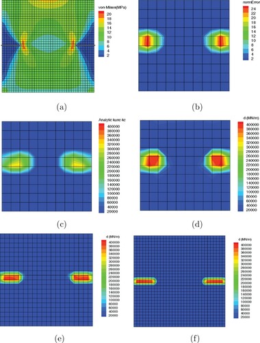
Figure 5. Square plate with multiple cracks: geometry and boundary conditions; center solid lines show the cracks in the first and second parts of the problem, dashed short lines (curves) show the crack pattern in the final part of the problem.

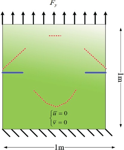
In the first part, a mesh grid with $10\times 10$ elements is used for crack detection. A finite element model with the same mesh size is used as the uncracked body. The plate contains two edge cracks with length a = 0.2 m on the left and right sides. The regularization parameters are assumed to be ${\alpha }_0={10}^{-7}$, ${\beta }_0=1000$ and a uniformly distributed random noise of $1\mathrm{\%}$ is applied to the measured responses of the cracked body model. Figure 6(a) shows the von-Mises stress contour in the cracked body model which is solved by X-FEM; cracks are shown with grey lines. Figure 6(b) presents the contour of residual error norm err, in the body; it is obvious that the CDRE method correctly detects both edge cracks. Figure 6(c,d) show the analytic and calculated stiffness reductions; the analytic stiffness matrix of the cracked body is calculated based on Equation (16(16) ${\mathbf{K}}_c={\mathbf{K}}_{ss}-{\mathbf{K}}_{se}{\mathbf{K}}_{ee}^{-1}{\mathbf{K}}_{es}$(16) ), from which the analytic stiffness reduction is obtained as $diag({\mathbf{K}}_{unc}-{\mathbf{K}}_c)$. The analytic and calculated stiffness reductions are in good agreement; however, some mismatches are observed in the cracked area. It is evident that the CDSR method detects the cracks correctly and provides an acceptable estimate for the stiffness matrix. In order to investigate the effect of detection grid size on the accuracy, two meshes with $20\times 20$ and $30\times 30$ elements are also studied. It is evident from Figure 6(e,f) that the finer the detection grid, the more accurate the locations of the cracks.

Figure 6. Square plate with two edge cracks, noise $1\mathrm{\%}$, ${\alpha }_0={10}^{-7}$ and ${\beta }_0=1000$ (a) von-Mises stress contour in the cracked body model, (b) err contour based on the CDRE method, (c) analytic X-FEM stiffness reduction $diag({\mathbf{K}}_{unc}-{\mathbf{K}}_c)$, (d) calculated stiffness reduction vector $\mathbf{d}$ based on the CDSR method, (e) calculated stiffness reduction vector $\mathbf{d}$ based on the CDSR method for $20\times 20$ detection mesh, (f) calculated stiffness reduction vector $\mathbf{d}$ based on the CDSR method for $30\times 30$ detection mesh.

In the second part, the robustness of the proposed methods under different noise levels is investigated. For this purpose, noise intensities of $5\mathrm{\%}$, $10\mathrm{\%}$ and $20\mathrm{\%}$ are applied to $\ddot{\mathbf{u}}$ and $\mathbf{u}$ responses based on Equation (32(32) $\begin{array}{rl}& {\hat{u}}_i=u_i(1+amp.\mathrm{{\rm Y}})\\ & {\hat{\ddot{u}}}_i={\ddot{u}}_i(1+amp.\mathrm{{\rm Y}})\end{array}$(32) ). Figure 7(a–c) demonstrate the performance of CDRE method; it is observed that the method correctly captures the edge cracks, however with the increasing noise level, some artefacts pollute the error norm contour. As it is expected, the absolute value of the error norm increases with noise growth. The noise effect on the CDSR method performance is shown in Figure 7(d–f); in this simulation, ${\alpha }_0={10}^{-7}$ was employed. The method detects the edge cracks but the solution error is significant in the high noise level of $20\mathrm{\%}$. It is well established in inverse problems' literature [40] that with the increase in noise to signal ratio, ill-posedness of the problem is magnified and thus the regularization parameter must be increased. This is investigated in Figure 7(g–i), where a value of ${\alpha }_0={10}^{-5}$ is assumed. It is observed that the solution quality is highly improved and the results are much closer to the analytic solution (Figure 6(c)).

Figure 7. Effect of noise level, $\alpha ={10}^{-7}$ and ${\beta }_0=1000$, (a, d and g) $5\mathrm{\%}$ noise, (b, e and h) $10\mathrm{\%}$ noise, (c, f and i) $20\mathrm{\%}$ noise; top row: the CDRE method, middle row: the CDSR method with ${\alpha }_0={10}^{-7}$, bottom row: the CDSR method with ${\alpha }_0={10}^{-5}$.

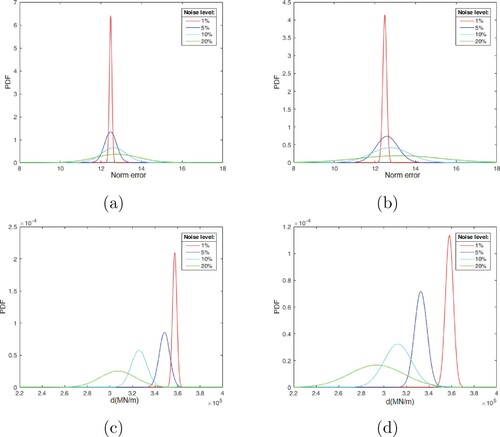
Since noise is random in nature, a probabilistic analysis is also performed to investigate its effects on the proposed crack detection strategies. For this purpose, the values of err in CDRE, and d in CDSR methods are calculated for different realizations of noise at point A that is marked in Figure 7(a); point A is close to crack and has high damage values. Random values of $\ddot{\mathbf{u}}$ and $\mathbf{u}$ responses are generated based on Equation (32(32) $\begin{array}{rl}& {\hat{u}}_i=u_i(1+amp.\mathrm{{\rm Y}})\\ & {\hat{\ddot{u}}}_i={\ddot{u}}_i(1+amp.\mathrm{{\rm Y}})\end{array}$(32) ); two random generators with uniform distribution, $\mathrm{{\rm Y}}\sim \mathcal{U}(-1,1)$ and Normal distribution, $\mathrm{{\rm Y}}\sim \mathcal{N}(0,1)$ were considered with noise amplitudes of $1\mathrm{\%},5\mathrm{\%},10\mathrm{\%}$ and $20\mathrm{\%}$. By trial and error, a sample size of 100 was selected for the study and histograms of the calculated values of err and d suggested a Normal distribution for the damage values. The results of the analysis are presented in Figure 8; it is observed that the damage probability distribution is almost identical for both noise distributions, however as expected, the normal noise distribution introduces more uncertainty to the solution. It is also observed that for both noise distributions and both damage measures as the noise amplitude is increased the damage distribution flattens and thus the uncertainty in the damage value increases. It seems that the proposed algorithms work satisfactory up to a noise amplitude of $10\mathrm{\%}$ but as expected the results deteriorate with the increase in noise amplitude.

Figure 8. Probabilistic study of noise effect on damage values at point A (Shown in Figure 7(a)), $\alpha ={10}^{-7}$ and $\beta =1000$: (a and c) noise with uniform distribution, (b and d) noise with normal distribution; top row: CDRE's err value, bottom row: CDSR's d value.

In the final part, the performance of the methods is investigated in the case of more complex cracks. As Figure 9(a) shows, two ${45}^{\circ }$ inclined edge cracks with length of $a=0.2\sqrt{2}$m, one short straight crack with length of a = 0.1 m and an arbitrary curved crack, are considered in the body. Figure 9(b), shows the error norm contour; it is observed that the CDRE method correctly detects the inclined and curved cracks, but can not completely capture the short crack and only a shadow is visible; a better detection might be possible with another detection grid or a different loading scenario. Figure 9(c,d) show the analytic stiffness reduction and calculated stiffness reduction $\mathbf{d}$ by the CDSR method, respectively. It is observed that the CDSR method can correctly capture all the cracks and the identified stiffness matrix is in good agreement with the analytic solution; considering the rank deficiency of the system equations, the existing small discrepancy seems acceptable.

Figure 9. Square plate with four cracks, noise $1\mathrm{\%}$, ${\alpha }_0={10}^{-7}$ and ${\beta }_0=1000$ (a) von-Mises stress contour in the cracked body model, (b) err contour based on the CDRE method, (c) analytic X-FEM stiffness reduction $diag({\mathbf{K}}_{unc}-{\mathbf{K}}_c)$, (d) calculated stiffness reduction vector $\mathbf{d}$ based on the CDSR method.

One of the main advantages of the proposed methods is that the number of cracks does not have any notable effect on the accuracy of solutions and the computational cost.

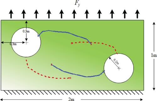
4.2. Rectangular plate with double holes and multiple cracks

The second example is devised to investigate the performance of the proposed methods in more complex geometries. The problem consists of a $2\mathrm{m}\times 1\mathrm{m}$ plate with two holes and multiple cracks; the holes are 0.2 m in radius. The material properties are the same as the previous example and the plate is in plane strain state. Figure 10 shows the problem geometry and boundary conditions. The bottom edge is fixed and uniform traction is applied to the top edge in y direction; the traction intensity varies from 0 to 0.01 MN m${}^{-1}$ in 0.1 s. The time step in numerical calculations is considered to be $\mathrm{\Delta }t=0.01$ s. The regularization parameters are selected as ${\beta }_0=1000$ and ${\alpha }_0={10}^{-7}$. An X-FEM model with 7200 bilinear quadrilateral elements is used as the cracked body and the detection grid mesh has 314 elements with 370 nodes. A noise level of $1\mathrm{\%}$ is applied to the responses.

Figure 10. Rectangular plate with double holes: geometry and boundary conditions; solid curves show the crack pattern in the first part of the problem and dashed curves show the crack pattern in the second part of the problem.

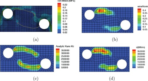
In the first part, two cracks are considered which emanate from the two holes and extend into the middle of the plate (solid curves in Figure 10). Figure 11(a) shows the von-Mises stress contour in the cracked body. The error norm contour in Figure 11(b) shows that the CDRE method detects the cracks almost perfectly. Figure 11(c,d) present the analytical and calculated stiffness reductions; it is observed that the CDSR method follows the cracks precisely and provides a good estimate of the stiffness matrix. One of the general observations from the numerical simulations is that the cracks which are closer to the load application locations, and which experience larger displacements, have a higher chance to be detected more precisely.

Figure 11. Rectangular plate with two holes and cracks, noise $1\mathrm{\%}$, ${\alpha }_0={10}^{-7}$ and ${\beta }_0=1000$ (a) von-Mises stress contour in the cracked body model, (b) err contour based on the CDRE method, (c) analytic X-FEM stiffness reduction $diag({\mathbf{K}}_{unc}-{\mathbf{K}}_c)$, (d) calculated stiffness reduction vector $\mathbf{d}$ based on the CDSR method.

In the second part, the same problem is solved for another crack configuration in which the cracks emanate vertically from the holes and then extend to the middle of the plate (dashed curves in Figure 10). Figure 12(a) presents the von-Mises stress contour in the cracked body and the performance of the CDRE method is shown in Figure 12(b); it is observed that error norm detects the cracks correctly; however, the vertical branches of the cracks are not perfectly captured. This might be due to the fact that these parts are normal to the load application direction, which makes the detection difficult. As Figure 12(d) shows the CDSR method fails to identify the cracks perfectly and only some shadows are observed. This shows that the regularization parameter is high in this simulation. 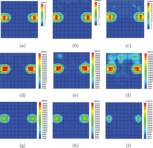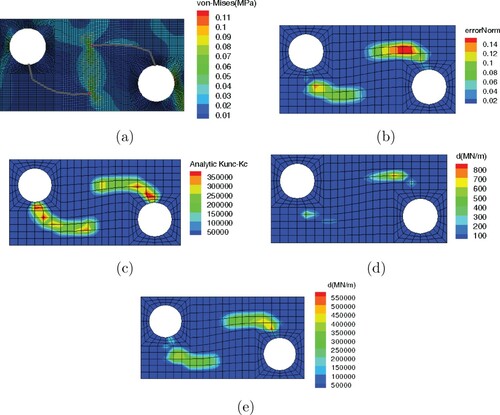Reducing ${\alpha }_0$ to ${10}^{-15}$ improves the solutions significantly (Figure 12(e)). Compared with the analytic solution, Figure 12(c), the identified stiffness matrix is almost accurate apart from a few regions in the vicinity of the right hole. The problem with the vertical branches is still observed in this simulation.

Figure 12. Rectangular plate with two holes and cracks, noise $1\mathrm{\%}$ and ${\beta }_0=1000$ (a) von-Mises stress contour in the cracked body model, (b) err contour based on the CDRE method, (c) analytic X-FEM stiffness reduction $diag({\mathbf{K}}_{unc}-{\mathbf{K}}_c)$, (d) calculated stiffness reduction vector $\mathbf{d}$ based on the CDSR method for ${\alpha }_0={10}^{-7}$, (e) calculated stiffness reduction vector $\mathbf{d}$ based on the CDSR method for ${\alpha }_0={10}^{-15}$.

4.3. The concrete portal frame with multiple cracks

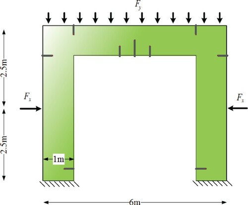
The purpose of the third example is to show the application of the proposed methods in more realistic situations. The problem consists of a $6m\times 4m$ portal frame that is in plane strain state. The material properties are that of unreinforced concrete with a Young's modulus of E = 25 GPa, Poisson's ratio of $\nu =0.3$ and density of 2400 kg m${}^{-3}$. Figure 13 shows the problem geometry and boundary conditions; the end of columns are fixed, uniform traction is applied to the beam in negative y direction and two concentrated forces are applied to the midspan of the columns in x direction. Since concrete is weak and cracks in tension, the crack pattern is chosen to somehow resemble the observed tensile and shear cracks in real concrete structures. The time step in numerical calculations is considered to be $\mathrm{\Delta }t=0.01$ s. The regularization parameters are selected as ${\beta }_0=1000$ and ${\alpha }_0={10}^{-7}$. An X-FEM model with 1892 bilinear quadrilateral elements is used as the cracked body model and the detection grid mesh has 153 elements. A noise level of $1\mathrm{\%}$ is applied to the responses.

Figure 13. Concrete portal frame: geometry and boundary conditions; cracks are shown with grey short lines.

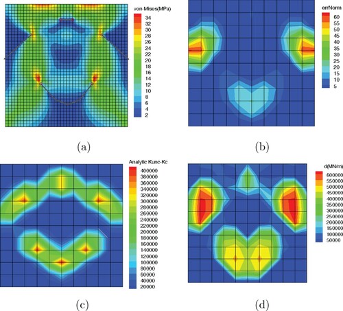
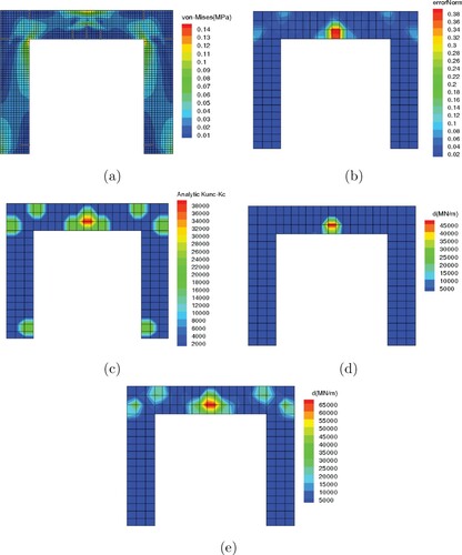
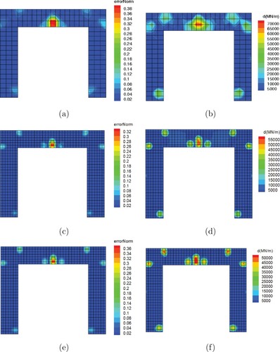
In the first part, crack detection is performed considering only the gravity load. It is assumed that $F_y$ varies from 0 to 0.01 MN m${}^{-1}$ in 0.1 s and the lateral loads are zero. Figure 14(a) shows the von-Mises stress contour of the cracked body; the effect of crack pattern on the stress distribution is evident. Figure 14(b) represents the error norm contour; it is observed that the CDRE method detects the tensile cracks in the beam and on top of the columns. However, the cracks at the bottom of the columns are not identified. The analytic X-FEM stiffness reduction in Figure 14(c) represents the expected detection result clearly. As Figure 14(d) demonstrates, the CDSR method only detects the cracks in the midspan of the beam; it seems that the regularization parameter is high; reducing ${\alpha }_0$ to ${10}^{-8}$ improves the detection result (Figure 14(e)); however, the cracks at the bottom of columns are not visible to the method.

Figure 14. Concrete portal frame with multiple cracks under gravity load, noise $1\mathrm{\%}$ and ${\beta }_0=1000$ (a) von-Mises stress contour in the cracked body model, (b) err contour based on the CDRE method, (c) analytic X-FEM stiffness reduction $diag({\mathbf{K}}_{unc}-{\mathbf{K}}_c)$, (d) calculated stiffness reduction vector $\mathbf{d}$ based on the CDSR method for ${\alpha }_0={10}^{-7}$ (e) calculated stiffness reduction vector $\mathbf{d}$ based on the CDSR method for ${\alpha }_0={10}^{-8}$.

In the second part, the frame is subjected to horizontal and gravity loads simultaneously. The concentrated load $F_x$ varies from 0 to 0.01 MN in 0.1 s and the gravity load is the same as the previous section. As Figure 15(a) shows, the CDRE method successfully detects all cracks in the frame. The same observation holds for the CDSR method (Figure 15(b)). In this example, it is observed that for both methods, the crack detection contours are diffused and cracks are not detected separately; this is more evident in the densely cracked region of the beam midspan. This problem can be attributed to the fact that the detection resolution is not enough to detect the cracks which are closely located and only a large diffused region is identified. To elaborate more on this issue, numerical simulations were performed with a finer detection mesh that had 623 bilinear elements. As Figure 15(c,d) show, with a fine detection mesh, all cracks are separately detected for both CDRE and CDSR methods and the contours are less diffused. In fact, the grid refinement increases the resolution of the detection methods and cracks are more precisely detected. In addition, the effect of similar meshes for both ”cracked body” and "uncracked body" is also investigated. As Figure 15(e,f) indicate, when the cracked body mesh is identical to the detection mesh, the accuracy of the method is increased and the effect of noise and error is less significant. This can be more evident by comparing the beam region in Figure 15(d,f).

Figure 15. Concrete portal frame with multiple cracks under gravity and horizontal loads, noise $1\mathrm{\%}$, ${\alpha }_0={10}^{-8}$ and ${\beta }_0=1000$ (a,c and e) err contour based on the CDRE method, (b,d and f) calculated stiffness reduction vector $\mathbf{d}$ based on the CDSR method. Top row: Coarse detection mesh; middle row: fine detection mesh; bottom row: similar detection and cracked body meshes.

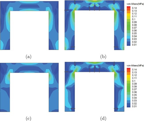
One important observation from the previous section was that the loading scenario has an important effect on the detection accuracy. This issue is mostly related to the problem of detectability. In order to detect the characteristics of a system from its responses, enough, meaningful and independent response data must be acquired; this is true for any detection method. For example, in order to detect the second mode shape and second frequency of a structure under dynamic loading, a loading which excites the second mode of vibration must be applied. Similarly, in this example, the gravity load alone does not provide enough responses for the detection of the column bottom cracks. This can also happen when the cracks do not alter the displacement and acceleration fields of the structure significantly. In fact, the proposed methods can detect the cracks which have determinative effects on the displacement and acceleration fields. If the cracks are so small that their effects diminish within a very small region around them, due to Saint Venant's principle, they may not have large enough effects compared to the system error and noise (i.e. noise to signal ratio) on the responses of the detection grid points and hence from the methods' view point, they have no effect and are not detected. To elaborate more on this issue, the displacement field contours of gravity and gravity+horizontal load cases for the cracked body and uncracked body are presented in Figure 16. As Figure 16(a,b) show, under the gravity load, cracks in the beam region have a significant effect on the displacement field; this is more pronounced in the midspan of the beam. In contrast, the displacement field in the column bottom region is unaffected by the cracks and it is almost the same for the cracked body and uncracked body. As Figure 16(c,d) suggest, when horizontal loads are also applied, the displacement fields change. In this case, the displacement field in the column bottom region is significantly different for the cracked body and the uncracked body and the method has a better chance to detect the cracks. This issue can be best observed by comparing the von-Mises stress contours for the two load cases. As Figure 17 (a,b) show, under gravity only loading, the von-Mises stress contour is almost the same for the cracked body and uncracked body. However, the difference is significant under gravity+horizontal loading (Figure 17(c,d)).

Figure 16. Contour of displacement in y direction: (a and c) uncracked body, (b and d) cracked body; top row: gravity load only, bottom row: gravity+horizontal load.

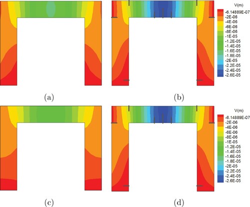
Figure 17. von-Mises contour: (a and c) uncracked body, (b and d) cracked body; top row: gravity load only, bottom row: gravity+horizontal load.

5. Conclusions

Two novel methods were presented for multiple crack detection in 2D solids. The methods were based on the insights from X-FEM formulation. The CDRE method employed the residual error norm to located the cracks and the CDSR method compared the stiffness matrix of the cracked body and uncracked body to find the dofs which are close to the cracks. The stiffness identification of the cracked body was based on a modified Tikhonov method with a variable regularization parameter, that used the CDRE technique. The sparsity structure of the cracked body stiffness matrix was assumed to be the same as the cracked body to increase computational efficiency. Several numerical examples were proposed to show the accuracy and robustness of the presented methods. The following observations were made: the computational costs of the proposed methods were much less than conventional crack detection strategies like metaheuristic optimization techniques. The number of cracks did not have a significant effect on the computational cost and accuracy. Cracks with different sizes, shapes, and orientations were precisely detected. Along with crack detection, the CDSR method provided an estimate for the stiffness matrix of the cracked body which could be used to find other system properties like frequencies and mode shapes. The methods were noise-robust; the detection was almost successful in the presence of high noise levels. One of our goals in the future works will be to extend the proposed methods into 3D problems with limited data acquisition on the surface. The most important challenge in this process is that the problem changes from a linear identification inverse problem into a nonlinear counterpart which requires special solution strategies.

Disclosure statement

No potential conflict of interest was reported by the author(s).

References

- Li H-N, Ren L, Jia Z-G, et al. State-of-the-art in structural health monitoring of large and complex civil infrastructures. J Civ Struct Health Monit. 2016;6(1):3–16.
- Mesquita E, Antunes P, Coelho F, et al. Global overview on advances in structural health monitoring platforms. J Civ Struct Health Monit. 2016;6(3):461–475.
- Dorafshan S, Maguire M. Bridge inspection: human performance, unmanned aerial systems and automation. J Civ Struct Health Monit. 2018;8(3):443–476.
- Gulizzi V, Rizzo P, Milazzo A, et al. An integrated structural health monitoring system based on electromechanical impedance and guided ultrasonic waves. J Civ Struct Health Monit. 2015;5(3):337–352.
- Cartz L. Nondestructive testing. Cleveland, OH: ASM International; 1995.
- Belytschko T, Black T. Elastic crack growth in finite elements with minimal remeshing. Int J Numer Meth Engng. 1999;45(5):601–620.
- Moës N, Sukumar N, Moran B, et al. An extended finite element method (x-fem) for two-and three-dimensional crack modeling. European Congress on Computational Methods in Applied Sciences and Engineering; Barcelona, Spain: 2000.
- Moës N, Belytschko T. Extended finite element method for cohesive crack growth. Eng Fract Mech. 2002;69(7):813–833.
- Elguedj T, Gravouil A, Combescure A. A mixed augmented lagrangian-extended finite element method for modelling elastic–plastic fatigue crack growth with unilateral contact. Int J Numer Methods Eng. 2007;71(13):1569–1597.
- Broumand P, Khoei A. X-fem modeling of dynamic ductile fracture problems with a nonlocal damage-viscoplasticity model. Finite Elem Anal Des. 2015;99:49–67.
- Liu F, Borja RI. A contact algorithm for frictional crack propagation with the extended finite element method. Int J Numer Methods Eng. 2008;76(10):1489–1512.
- Khoei A, Mousavi ST. Modeling of large deformation–large sliding contact via the penalty x-fem technique. Comput Materials Sci. 2010;48(3):471–480.
- Broumand P, Khoei A. General framework for dynamic large deformation contact problems based on phantom-node x-fem. Comput Mech. 2018;61(4):449–469.
- Khoei A, Vahab M, Haghighat E, et al. A mesh-independent finite element formulation for modeling crack growth in saturated porous media based on an enriched-fem technique. Int J Fract. 2014;188(1):79–108.
- Khoei A, Vahab M, Hirmand M. Modeling the interaction between fluid-driven fracture and natural fault using an enriched-fem technique. Int J Fract. 2016;197(1):1–24.
- Sawada T, Tezuka A. Llm and x-fem based interface modeling of fluid–thin structure interactions on a non-interface-fitted mesh. Comput Mech. 2011;48(3):319–332.
- Khoei A. Extended finite element method : theory and applications. Chichester, UK: John Wiley & Sons, Ltd.; 2015.
- Rabinovich D, Givoli D, Vigdergauz S. Xfem-based crack detection scheme using a genetic algorithm. Int J Numer Methods Eng. 2007;71(9):1051–1080.
- Waisman H, Chatzi E, Smyth AW. Detection and quantification of flaws in structures by the extended finite element method and genetic algorithms. Int J Numer Methods Eng. 2010;82(3):303–328.
- Sun H, Waisman H, Betti R. Nondestructive identification of multiple flaws using xfem and a topologically adapting artificial bee colony algorithm. Int J Numer Methods Eng. 2013;95(10):871–900.
- Nanthakumar S, Lahmer T, Zhuang X, et al. Detection of material interfaces using a regularized level set method in piezoelectric structures. Inverse Probl Sci Eng. 2016;24(1):153–176.
- Agathos K, Chatzi E, Bordas SP. Multiple crack detection in 3d using a stable xfem and global optimization. Comput Mech. 2018;62:835–852.
- Khatir S, Wahab MA. A computational approach for crack identification in plate structures using xfem, xiga, pso and jaya algorithm. Theoretical Appl Fract. 2019;103:102240.
- Khaji N. Crack detection in 2d domains using extended finite element method and particle swarm optimization. Modares Civil Eng J. 2017;16(20):177–189.
- Livani M, Khaji N, Zakian P. Identification of multiple flaws in 2d structures using dynamic extended spectral finite element method with a universally enhanced meta-heuristic optimizer. Struct Multidiscipl Optim. 2018;57(2):605–623.
- Köppen M. Crack identification using extended isogeometric analysis and particle swarm optimization. Proceedings of the 7th International Conference on Fracture Fatigue and Wear: FFW 2018, 9-10 July 2018, Ghent University; Belgium: Springer; 2018. p. 210.
- Fang S-E, Perera R. A response surface methodology based damage identification technique. Smart Mater Struct. 2009;18(6):065009.
- Mukhopadhyay T, Chowdhury R, Chakrabarti A. Structural damage identification: a random sampling-high dimensional model representation approach. Adv Struct Eng. 2016;19(6):908–927.
- Mukhopadhyay T. A multivariate adaptive regression splines based damage identification methodology for web core composite bridges including the effect of noise. J Sandwich Struct Mater. 2018;20(7):885–903.
- Jung J, Taciroglu E. Modeling and identification of an arbitrarily shaped scatterer using dynamic xfem with cubic splines. Comput Meth Appl Mech Eng. 2014;278:101–118.
- Chan T, Li J, Caprani C. Structural identification and evaluation for shm applications. J Civ Struct Health Monit. 2018;8(5):719–720.
- Fritzen C-P. Identification of mass, damping, and stiffness matrices of mechanical systems. J Vibration Acoustics Stress and Reliability Design. 1986;108(1):9–16.
- Cheng L, Tian GY. Surface crack detection for carbon fiber reinforced plastic (cfrp) materials using pulsed eddy current thermography. IEEE Sens J. 2011;11(12):3261–3268.
- Siavashi M, Kowsary F, Abbasi-Shavazi E. Detection of flaws in a two-dimensional body through measurement of surface temperatures and use of conjugate gradient method. Comput Mech. 2010;46(4):597–607.
- Koh CG, See LM, Balendra T. Estimation of structural parameters in time domain: a substructure approach. Earthq Eng Struct Dyn. 1991;20(8):787–801.
- Brincker R, Zhang L, Andersen P. Modal identification of output-only systems using frequency domain decomposition. Smart Materials and Struct. 2001;10(3):441.
- Mahato S, Chakraborty A. Sequential clustering of synchrosqueezed wavelet transform coefficients for efficient modal identification. J Civ Struct Health Monit. 2019;9(2):271–291.
- Cao L, Liu J, Xu C, et al. Uncertain inverse method by the sequential fosm and its application on uncertainty reconstruction of vehicle–pedestrian collision accident. Int J Mech Mater Des. 2020;1:1–14.
- Zhu X, Law S-S. Recent developments in inverse problems of vehicle–bridge interaction dynamics. J Civ Struct Health Monit. 2016;6(1):107–128.
- Muelller JL, Siltanen S. Linear and nonlinear inverse problems with practical applications. Vol. 1. Philadelphia, Pennsylvania: Siam; 2012.
- Mera N, Elliott L, Ingham D. A multi-population genetic algorithm approach for solving ill-posed problems. Comput Mech. 2004;33(4):254–262.
- Chen K, Kao J, Chen J, et al. Desingularized meshless method for solving Laplace equation with over-specified boundary conditions using regularization techniques. Comput Mech. 2009;43(6):827–837.
- Osher S, Burger M, Goldfarb D, et al. An iterative regularization method for total variation-based image restoration. Multiscale Model Simul. 2005;4(2):460–489.
- Liu J, Sun X, Han X, et al. Dynamic load identification for stochastic structures based on Gegenbauer polynomial approximation and regularization method. Mech Syst Signal Process. 2015;56:35–54.
- Liu J, Sun X, Meng X, et al. A novel shape function approach of dynamic load identification for the structures with interval uncertainty. Int J Mech Mater Des. 2016;12(3):375–386.
- Babuška I, Melenk JM. The partition of unity method. Int J Numer Methods Eng. 1997;40(4):727–758.
- Broumand P, Khoei A. The extended finite element method for large deformation ductile fracture problems with a non-local damage-plasticity model. Eng Fract Mech. 2013;112:97–125.
- Sutton MA, Orteu JJ, Schreier H. Image correlation for shape, motion and deformation measurements: basic concepts, theory and applications. Columbia, South Carolina: Springer Science & Business Media; 2009.
- Pierron F, Forquin P. Ultra-high-speed full-field deformation measurements on concrete spalling specimens and stiffness identification with the virtual fields method. Strain. 2012;48(5):388–405.