Inverse eigenvalue problems for discrete gyroscopic systems

Abstract

A discrete gyroscopic system is characterized by $2n$ first-order ordinary differential equations defined by one symmetric and one skew-symmetric, which system describes the motion of a spinning body containing elastic parts. In this paper, we consider the inverse problems of such system: Given partial spectral data, find a system such that it is of the desired spectral data. The general solution of the problem is given and the best approximation solution to a pair of matrices is provided by QR-decomposition and matrix derivation. In addition, we also consider a special case in which the system operates below the lowest critical speed. The numerical examples show that the proposed method is effective.

Keywords:

• Discrete gyroscopic system
• matrix equation
• inverse problem
• measured modal data
• optimal approximation

AMS subject classifications:

• 65F18
• 15A24

1. Introduction

With the rapid development of rotating spacecraft, gyroscopic systems and corresponding eigenvalue problems have been widely concerned [1–9]. Let us consider a discrete gyroscopic system described by $2n$ first-order differential equations being of the following matrix form: (1) $J_a\dot{\mathit{x}}\left(t\right)+G_a\mathit{x}\left(t\right)=\mathit{f}\left(t\right),$(1) where $J_a$ is a $2n\times 2n$ real symmetric matrix, and $G_a$ is a $2n\times 2n$ real skew-symmetric matrix, $\mathit{x}\left(t\right)$ is a $2n$-dimensional state vector, and $\mathit{f}\left(t\right)$ is a $2n$-dimensional force vector. It is known that the eigenvalue problem associated with Equation (1(1) $J_a\dot{\mathit{x}}\left(t\right)+G_a\mathit{x}\left(t\right)=\mathit{f}\left(t\right),$(1) ) is $({\lambda }_r{J}_a+G_a){\mathit{x}}_r=\mathbf{0},r=1,2,\dots ,2n,$ where the scalars ${\lambda }_r(r=1,2,\dots ,2n)$ and nonzero vectors ${\mathit{x}}_r(r=1,2,\dots ,2n)$ are, respectively, called the eigenvalues and eigenvectors of the system. If $J_a$ is symmetric and positive definite and $G_a$ is skew-symmetric, then the eigenvalues are all pure imaginary and complex conjugate, and the eigenvectors are also complex conjugate.

The system described by Equation (1(1) $J_a\dot{\mathit{x}}\left(t\right)+G_a\mathit{x}\left(t\right)=\mathit{f}\left(t\right),$(1) ) belongs to the general class of linear gyroscopic systems, which is related to the small oscillation of systems about steady motion. A common example is the motion of a spinning rigid body with elastically connected parts. If the system operates below the lowest critical speed, in this case, the matrix $J_a$ is symmetric and positive definite. We note that a special class of conservative gyroscopic systems can be easily transformed into such systems. In fact, the equations of motion of a conservative gyroscopic system can be written in the following matrix form: (2) ${\tilde{M}}_a\ddot{\mathit{q}}\left(t\right)+{\tilde{G}}_a\dot{\mathit{q}}\left(t\right)+{\tilde{K}}_a\mathit{q}\left(t\right)=\mathit{u}\left(t\right),$(2) where $\mathit{q}\left(t\right)$ represents the generalized coordinates of the system, ${\tilde{M}}_a,{\tilde{G}}_a$ and ${\tilde{K}}_a$ are called the analytical mass, gyroscopic and stiffness matrices, respectively, and $\mathit{u}\left(t\right)$ is force vector. The solution of Equation (2(2) ${\tilde{M}}_a\ddot{\mathit{q}}\left(t\right)+{\tilde{G}}_a\dot{\mathit{q}}\left(t\right)+{\tilde{K}}_a\mathit{q}\left(t\right)=\mathit{u}\left(t\right),$(2) ) can be conveniently obtained by transforming it into a first-order vector equation. For this purpose, we introduce the state vector $\mathit{x}\left(t\right)$ and the corresponding force vector $\mathit{f}\left(t\right)$ defined by $\mathit{x}\left(t\right)=\left[\dot{\mathit{q}}\right(t{)}^{\mathrm{\top }},\mathit{q}(t{)}^{\mathrm{\top }}{]}^{\mathrm{\top }},\mathit{f}(t)=[\mathit{u}(t{)}^{\mathrm{\top }},{\mathbf{0}}^{\mathrm{\top }}{]}^{\mathrm{\top }},$ as well as the $2n\times 2n$ matrices $J_a=\left[\begin{array}{cc}{\tilde{M}}_a& 0\\ 0& {\tilde{K}}_a\end{array}\right],G_a=\left[\begin{array}{cc}{\tilde{G}}_a& {\tilde{K}}_a\\ -{\tilde{K}}_a& 0\end{array}\right].$ Thus, Equation (2(2) ${\tilde{M}}_a\ddot{\mathit{q}}\left(t\right)+{\tilde{G}}_a\dot{\mathit{q}}\left(t\right)+{\tilde{K}}_a\mathit{q}\left(t\right)=\mathit{u}\left(t\right),$(2) ) is equivalently rewritten as Equation (1(1) $J_a\dot{\mathit{x}}\left(t\right)+G_a\mathit{x}\left(t\right)=\mathit{f}\left(t\right),$(1) ).

In general, the system (1) is modelled in a highly idealized state and may not truly describe all the physical aspects of a real-life vibrating structure. There must be significant differences between the analytical predictions and the measured results, so we need to update the model by using the measured modal data (eigenvalues and eigenvectors). Mathematically, the problem of updating $J_a$ and $G_a$ simultaneously can be formulated as the following inverse problems.

Problem I

Let $\mathrm{\Lambda }=\text{diag}\{{\lambda }_1,{\lambda }_2,\dots ,{\lambda }_{2m}\}\in {\mathbb{C}}^{2m\times 2m}$, $X=[{\mathit{x}}_1,{\mathit{x}}_2,\dots ,{\mathit{x}}_{2m}]\in {\mathbb{C}}^{2n\times 2m}$ be the measured eigenvalue and eigenvector matrices, where diagonal elements of Λ are all distinct and purely imaginary, X is of full column rank $2m$, and both Λ and X are closed under complex conjugation, namely, ${\lambda }_{2j}={\overline{\lambda }}_{2j-1}\in \mathbb{C},{\mathit{x}}_{2j}={\overline{\mathit{x}}}_{2j-1}\in {\mathbb{C}}^{2n},$ $j=1,2,\dots ,m$. Find $(\hat{J},\hat{G})\in {\zeta }_E$ such that $\parallel \hat{J}-J_a{\parallel }^2+\parallel \hat{G}-G_a{\parallel }^2=\underset{(J,G)\in {\zeta }_E}{min}\left(\parallel J-J_a{\parallel }^2+\parallel G-G_a{\parallel }^2\right),$ where ${\zeta }_E=\left\{\right(J,G)\in {\mathbb{S}\mathbb{R}}^{2n\times 2n}\times {\mathbb{S}\mathbb{S}\mathbb{R}}^{2n\times 2n}|JX\mathrm{\Lambda }+GX=0\}.$

Problem II

Let $\mathrm{\Lambda }=\text{diag}\{{\lambda }_1,{\lambda }_2,\dots ,{\lambda }_{2m}\}\in {\mathbb{C}}^{2m\times 2m}$, $X=[{\mathit{x}}_1,{\mathit{x}}_2,\dots ,{\mathit{x}}_{2m}]\in {\mathbb{C}}^{2n\times 2m}$ be the measured eigenvalue and eigenvector matrices, where diagonal elements of Λ are all distinct and purely imaginary, X is of full column rank $2m$, and both Λ and X are closed under complex conjugation. Find symmetric positive definite matrix J and real nonsingular skew-symmetric matrix G such that $JX\mathrm{\Lambda }+GX=0.$

The inverse eigenvalue problem for linear lumped parameter systems modelled by a vector differential equation of the form: $M\ddot{\mathbf{q}}\left(t\right)+D\dot{\mathbf{q}}\left(t\right)+K\mathbf{q}\left(t\right)=\mathbf{f}\left(t\right)$ has been considered by Lancaster and Maroulas [10], Lancaster and Ye [11], Starek et al. [12], and Starek and Inman [13–15]. Lancaster and Maroulas [10] have formulated a solution of the inverse eigenvalue problem by means of the spectral theory of matrix polynomials. Starek et al. [12] have solved the inverse spectral problem in the state-space form and defined the conditions for given spectral and modal data under which the inverse formulas determine real symmetric coefficient matrices $\tilde{D}:=M^{-\frac{1}{2}}D{M}^{-\frac{1}{2}}$ and $\tilde{K}:=M^{-\frac{1}{2}}K{M}^{-\frac{1}{2}}$. However, their solution requires that the given eigenvalues must all be complex-valued and does not preserve given eigenvectors. Starek and Inman [13] have derived the conditions under which spectral and modal data determine real symmetric coefficient matrices $\tilde{D}$ and $\tilde{K}$ for the case in which the eigenvalues may also be real valued corresponding to the existence of one or more overdamped modes. The paper by Starek and Inman [14] gives an alternative solution to the inverse problem solved in [12] and extends these results to ensure that the coefficient matrices will be both symmetric and positive definite. In [15], authors have provided an alternative solution to the inverse eigenvalue problem in vibration in $2n$ space and via matrix polynomial approach to include the design of nonproportional vibrating systems for given spectral and modal data.

The matrix model updating problems have been considered by many researchers (see Refs. [16–20] and references cited therein). However, the problems I and II have not been considered in the literature as far as we know.

Our main contribution is to provide the solvability conditions and give the general expressions of the solutions for the inverse eigenvalue problems I and II. By taking advantage of the proposed numerical method, the updated model has the following properties:

• The measured eigenvalues and eigenvectors will reproduce in the updated model.

• The symmetry of the updated matrices is preserved and the difference between the updated model and the original model is minimal.

Compared with the methods proposed by Starek and Inman to determine real symmetric coefficient matrices by the spectral decomposition of real-valued self-adjoint quadratic pencils, we observe that the approach in this paper for solving problems I and II by QR-decomposition and matrix derivation is fairly simple and easy to put in practice, and seems to have enough generality that, with some suitable modifications, it can be applied to other types of inverse problems as well.

Throughout this paper, we shall adopt the following notation. ${\mathbb{C}}^{m\times n}$ and ${\mathbb{R}}^{m\times n}$ denote the sets of all $m\times n$ complex and real matrices, respectively. ${\mathbb{S}\mathbb{R}}^{n\times n}$ and ${\mathbb{S}\mathbb{S}\mathbb{R}}^{n\times n}$ denote the sets of all symmetric matrices and skew-symmetric matrices in ${\mathbb{R}}^{n\times n}$. $A^{\mathrm{\top }}$ and $\mathrm{t}\mathrm{r}\left(A\right)$ stand for the transpose and the trace of a matrix A, respectively. If we define an inner product in ${\mathbb{R}}^{m\times n}$ by $〈A,B〉=\mathrm{t}\mathrm{r}\left(B^{\mathrm{\top }}A\right)$, $\mathrm{\forall }A,B\in {\mathbb{R}}^{m\times n}$. Then, the matrix norm $\parallel \cdot \parallel$ induced by the inner product is the Frobenius norm.

2. The solution of Problem I

In order to solve Problem I, we need the following lemma.

Lemma 2.1

[21, 22]

Let A, B be two real matrices, and X be an unknown variable matrix. Then $\begin{array}{rl}\frac{\mathrm{\partial }\mathrm{t}\mathrm{r}\left(BX\right)}{\mathrm{\partial }X}& =B^{\mathrm{\top }},\frac{\mathrm{\partial }\mathrm{t}\mathrm{r}\left(X{}^{\mathrm{\top }}B{}^{\mathrm{\top }}\right)}{\mathrm{\partial }X}=B^{\mathrm{\top }},\frac{\mathrm{\partial }\mathrm{t}\mathrm{r}\left(AXBX\right)}{\mathrm{\partial }X}=(BXA+AXB{)}^{\mathrm{\top }},\\ \frac{\mathrm{\partial }\mathrm{t}\mathrm{r}\left(A{X}^{\mathrm{\top }}B{X}^{\mathrm{\top }}\right)}{\mathrm{\partial }X}& =B{X}^{\mathrm{\top }}A+A{X}^{\mathrm{\top }}B,\frac{\mathrm{\partial }\mathrm{t}\mathrm{r}\left(AXB{X}^{\mathrm{\top }}\right)}{\mathrm{\partial }X}=AXB+A^{\mathrm{\top }}X{B}^{\mathrm{\top }}.\end{array}$

Define $T_{2m}$ as (3) $T_{2m}=\text{diag}\left\{\frac{1}{\sqrt{2}}\left[\begin{array}{cc}1& -i\\ 1& i\end{array}\right],\dots ,\frac{1}{\sqrt{2}}\left[\begin{array}{cc}1& -i\\ 1& i\end{array}\right]\right\}\in {\mathbb{C}}^{2m\times 2m},$(3) where $i=\sqrt{-1}$. It is easy to verify that $T_{2m}$ is a unitary matrix, that is, ${\overline{T}}_{2m}^{\mathrm{\top }}{T}_{2m}=I_{2m}$. Using this matrix, we have (4) $\begin{array}{rl}\tilde{\mathrm{\Lambda }}& ={\overline{T}}_{2m}^{\mathrm{\top }}\mathrm{\Lambda }{T}_{2m}=\text{diag}\left\{\left[\begin{array}{cc}0& {\text{β}}_1\\ -{\text{β}}_1& 0\end{array}\right],\dots ,\left[\begin{array}{cc}0& {\text{β}}_{2m-1}\\ -{\text{β}}_{2m-1}& 0\end{array}\right]\right\}\\ & \triangleq \text{diag}\{{\tilde{\mathrm{\Lambda }}}_1,\dots ,{\tilde{\mathrm{\Lambda }}}_m\}\in {\mathbb{R}}^{2m\times 2m},\end{array}$(4) (5) $\begin{array}{rl}\tilde{X}& =X{T}_{2m}=[\sqrt{2}{\mathit{y}}_1,\sqrt{2}{\mathit{z}}_1,\dots ,\sqrt{2}{\mathit{y}}_{2m-1},\sqrt{2}{\mathit{z}}_{2m-1}]\in {\mathbb{R}}^{2n\times 2m},\end{array}$(5) where ${\text{β}}_j$ is the imaginary part of the complex number ${\lambda }_j$, and ${\mathit{y}}_j$ and ${\mathit{z}}_j$ are, respectively, the real part and imaginary part of the complex vector ${\mathit{x}}_j$ for $j=1,3,\dots ,2m-1$. Using (4(4) $\begin{array}{rl}\tilde{\mathrm{\Lambda }}& ={\overline{T}}_{2m}^{\mathrm{\top }}\mathrm{\Lambda }{T}_{2m}=\text{diag}\left\{\left[\begin{array}{cc}0& {\text{β}}_1\\ -{\text{β}}_1& 0\end{array}\right],\dots ,\left[\begin{array}{cc}0& {\text{β}}_{2m-1}\\ -{\text{β}}_{2m-1}& 0\end{array}\right]\right\}\\ & \triangleq \text{diag}\{{\tilde{\mathrm{\Lambda }}}_1,\dots ,{\tilde{\mathrm{\Lambda }}}_m\}\in {\mathbb{R}}^{2m\times 2m},\end{array}$(4) ) and (5(5) $\begin{array}{rl}\tilde{X}& =X{T}_{2m}=[\sqrt{2}{\mathit{y}}_1,\sqrt{2}{\mathit{z}}_1,\dots ,\sqrt{2}{\mathit{y}}_{2m-1},\sqrt{2}{\mathit{z}}_{2m-1}]\in {\mathbb{R}}^{2n\times 2m},\end{array}$(5) ), the matrix equation $JX\mathrm{\Lambda }+GX=0$ can be written as (6) $J\tilde{X}\tilde{\mathrm{\Lambda }}+G\tilde{X}=0.$(6) Since $\mathrm{r}\mathrm{a}\mathrm{n}\mathrm{k}\left(X\right)=\mathrm{r}\mathrm{a}\mathrm{n}\mathrm{k}\left(\tilde{X}\right)=2m$, the QR-decomposition of $\tilde{X}$ is of the form: (7) $\tilde{X}=Q\left[\begin{array}{c}R\\ 0\end{array}\right]=[Q_1,Q_2]\left[\begin{array}{c}R\\ 0\end{array}\right],$(7) where Q is orthogonal with $Q_1\in {\mathbb{R}}^{2n\times 2m}$, and $R\in {\mathbb{R}}^{2m\times 2m}$ is nonsingular. Partition the parameter matrices $Q^{\mathrm{\top }}JQ$ and $Q^{\mathrm{\top }}GQ$ into blocks, (8) $Q^{\mathrm{\top }}JQ=\left[\begin{array}{cc}{J}_{11}& J_{12}\\ J_{12}^{\mathrm{\top }}& J_{22}\end{array}\right],Q^{\mathrm{\top }}GQ=\left[\begin{array}{cc}{G}_{11}& G_{12}\\ -G_{12}^{\mathrm{\top }}& G_{22}\end{array}\right],$(8) where $J_{11}$ and $G_{11}$ are real $2m\times 2m$ matrices. By (7(7) $\tilde{X}=Q\left[\begin{array}{c}R\\ 0\end{array}\right]=[Q_1,Q_2]\left[\begin{array}{c}R\\ 0\end{array}\right],$(7) ) and (8(8) $Q^{\mathrm{\top }}JQ=\left[\begin{array}{cc}{J}_{11}& J_{12}\\ J_{12}^{\mathrm{\top }}& J_{22}\end{array}\right],Q^{\mathrm{\top }}GQ=\left[\begin{array}{cc}{G}_{11}& G_{12}\\ -G_{12}^{\mathrm{\top }}& G_{22}\end{array}\right],$(8) ), Equation (6(6) $J\tilde{X}\tilde{\mathrm{\Lambda }}+G\tilde{X}=0.$(6) ) is equivalent to (9) $\left[\begin{array}{cc}{J}_{11}& J_{12}\\ J_{12}^{\mathrm{\top }}& J_{22}\end{array}\right]\left[\begin{array}{c}R\tilde{\mathrm{\Lambda }}\\ 0\end{array}\right]+\left[\begin{array}{cc}{G}_{11}& G_{12}\\ -G_{12}^{\mathrm{\top }}& G_{22}\end{array}\right]\left[\begin{array}{c}R\\ 0\end{array}\right]=0.$(9)

Then, it follows from Equation (9(9) $\left[\begin{array}{cc}{J}_{11}& J_{12}\\ J_{12}^{\mathrm{\top }}& J_{22}\end{array}\right]\left[\begin{array}{c}R\tilde{\mathrm{\Lambda }}\\ 0\end{array}\right]+\left[\begin{array}{cc}{G}_{11}& G_{12}\\ -G_{12}^{\mathrm{\top }}& G_{22}\end{array}\right]\left[\begin{array}{c}R\\ 0\end{array}\right]=0.$(9) ) that (10) $\begin{array}{rl}& J_{11}R\tilde{\mathrm{\Lambda }}+G_{11}R=0,\end{array}$(10) (11) $\begin{array}{rl}& J_{12}^{\mathrm{\top }}R\tilde{\mathrm{\Lambda }}-G_{12}^{\mathrm{\top }}R=0.\end{array}$(11) By Equation (10(10) $\begin{array}{rl}& J_{11}R\tilde{\mathrm{\Lambda }}+G_{11}R=0,\end{array}$(10) ) and $G_{11}$ being a skew-symmetric matrix implies that (12) $R^{\mathrm{\top }}{J}_{11}R\tilde{\mathrm{\Lambda }}=\tilde{\mathrm{\Lambda }}{R}^{\mathrm{\top }}{J}_{11}R.$(12) For simplicity, let (13) $R^{\mathrm{\top }}{J}_{11}R=\left[{\tilde{J}}_{ij}\right],i,j=1,\dots ,m,$(13) where ${\tilde{J}}_{ij}\in {\mathbb{R}}^{2\times 2},i,j=1,\dots ,m.$ When $i\ne j$, it follows from Equation (12(12) $R^{\mathrm{\top }}{J}_{11}R\tilde{\mathrm{\Lambda }}=\tilde{\mathrm{\Lambda }}{R}^{\mathrm{\top }}{J}_{11}R.$(12) ) that (14) ${\tilde{J}}_{ij}{\tilde{\mathrm{\Lambda }}}_j={\tilde{\mathrm{\Lambda }}}_i{\tilde{J}}_{ij},i,j=1,\dots ,m.$(14) Noting that ${\text{β}}_i\ne {\text{β}}_j$ for $i\ne j$, $i,j=1,3,\dots ,2m-1$, it follows from Equation (14(14) ${\tilde{J}}_{ij}{\tilde{\mathrm{\Lambda }}}_j={\tilde{\mathrm{\Lambda }}}_i{\tilde{J}}_{ij},i,j=1,\dots ,m.$(14) ) that (15) ${\tilde{J}}_{ij}=0,i,j=1,2,\dots ,m.$(15) When i = j, it follows from Equation (12(12) $R^{\mathrm{\top }}{J}_{11}R\tilde{\mathrm{\Lambda }}=\tilde{\mathrm{\Lambda }}{R}^{\mathrm{\top }}{J}_{11}R.$(12) ) that (16) ${\tilde{J}}_{jj}{\tilde{\mathrm{\Lambda }}}_j={\tilde{\mathrm{\Lambda }}}_j{\tilde{J}}_{jj},\mathrm{s}.\mathrm{t}.{\tilde{J}}_{jj}={\tilde{J}}_{jj}^{\mathrm{\top }},j=1,2,\dots ,m,$(16) which implies that (17) ${\tilde{J}}_{jj}=t_j{I}_2,j=1,2,\dots ,m,$(17) where $t_j,j=1,2,\dots ,m,$ are arbitrary real numbers. By (15(15) ${\tilde{J}}_{ij}=0,i,j=1,2,\dots ,m.$(15) ) and (17(17) ${\tilde{J}}_{jj}=t_j{I}_2,j=1,2,\dots ,m,$(17) ), the solution of Equation (10(10) $\begin{array}{rl}& J_{11}R\tilde{\mathrm{\Lambda }}+G_{11}R=0,\end{array}$(10) ) can be given by (18) $J_{11}=R^{-\mathrm{\top }}\text{diag}\{t_1{I}_2,t_2{I}_2,\dots ,t_m{I}_2\}{R}^{-1},G_{11}=-J_{11}R\tilde{\mathrm{\Lambda }}{R}^{-1}.$(18) If partition $R^{-1}$ by (19) $R^{-1}=\left[\begin{array}{c}{L}_1\\ L_2\\ ⋮\\ L_m\end{array}\right],$(19) where $L_i\in {\mathbb{R}}^{2\times 2m},i=1,2,\dots ,m.$ Then we can get (20) $J_{11}=t_1{M}_1+t_2{M}_2+\cdots +t_m{M}_m,G_{11}=-J_{11}R\tilde{\mathrm{\Lambda }}{R}^{-1},$(20) where $M_i=L_i^{\mathrm{\top }}{L}_i,i=1,2,\dots ,m$. It follows from Equation (11(11) $\begin{array}{rl}& J_{12}^{\mathrm{\top }}R\tilde{\mathrm{\Lambda }}-G_{12}^{\mathrm{\top }}R=0.\end{array}$(11) ) that (21) $G_{12}=-R^{-\mathrm{\top }}\tilde{\mathrm{\Lambda }}{R}^{\mathrm{\top }}{J}_{12},$(21)

where $J_{12}$ is an arbitrary real matrix. Substituting (20(20) $J_{11}=t_1{M}_1+t_2{M}_2+\cdots +t_m{M}_m,G_{11}=-J_{11}R\tilde{\mathrm{\Lambda }}{R}^{-1},$(20) ) and (21(21) $G_{12}=-R^{-\mathrm{\top }}\tilde{\mathrm{\Lambda }}{R}^{\mathrm{\top }}{J}_{12},$(21) ) into (8(8) $Q^{\mathrm{\top }}JQ=\left[\begin{array}{cc}{J}_{11}& J_{12}\\ J_{12}^{\mathrm{\top }}& J_{22}\end{array}\right],Q^{\mathrm{\top }}GQ=\left[\begin{array}{cc}{G}_{11}& G_{12}\\ -G_{12}^{\mathrm{\top }}& G_{22}\end{array}\right],$(8) ), we can obtain the following expression of the solution set ${\zeta }_E$: (22) ${\zeta }_E=\left\{(J,G)|J=Q\left[\begin{array}{cc}{J}_{11}& J_{12}\\ J_{12}^{\mathrm{\top }}& J_{22}\end{array}\right]Q^{\mathrm{\top }},G=Q\left[\begin{array}{cc}-J_{11}R\tilde{\mathrm{\Lambda }}{R}^{-1}& -R^{-\mathrm{\top }}\tilde{\mathrm{\Lambda }}{R}^{\mathrm{\top }}{J}_{12}\\ -J_{12}^{\mathrm{\top }}R\tilde{\mathrm{\Lambda }}{R}^{-1}& G_{22}\end{array}\right]Q^{\mathrm{\top }}\right\},$(22) where $J_{11}$ is given by (20(20) $J_{11}=t_1{M}_1+t_2{M}_2+\cdots +t_m{M}_m,G_{11}=-J_{11}R\tilde{\mathrm{\Lambda }}{R}^{-1},$(20) ), $J_{22}$ is an arbitrary symmetric matrix, $G_{22}$ is an arbitrary skew-symmetric matrix, and $J_{12}$ is an arbitrary matrix.

According to (22(22) ${\zeta }_E=\left\{(J,G)|J=Q\left[\begin{array}{cc}{J}_{11}& J_{12}\\ J_{12}^{\mathrm{\top }}& J_{22}\end{array}\right]Q^{\mathrm{\top }},G=Q\left[\begin{array}{cc}-J_{11}R\tilde{\mathrm{\Lambda }}{R}^{-1}& -R^{-\mathrm{\top }}\tilde{\mathrm{\Lambda }}{R}^{\mathrm{\top }}{J}_{12}\\ -J_{12}^{\mathrm{\top }}R\tilde{\mathrm{\Lambda }}{R}^{-1}& G_{22}\end{array}\right]Q^{\mathrm{\top }}\right\},$(22) ), we know that the solution set ${\zeta }_E$ is always nonempty and ${\zeta }_E$ is a closed convex subset, which implies that Problem I has a unique solution $(\hat{J},\hat{G})\in {\zeta }_E$ by the best approximation theorem [23]. For any pair of matrices $(J,G)\in {\zeta }_E$, we have $\begin{array}{rl}f(J,G)& =\parallel J-J_a{\parallel }^2+\parallel G-G_a{\parallel }^2\\ & ={∥Q\left[\begin{array}{cc}{J}_{11}& J_{12}\\ J_{12}^{\mathrm{\top }}& J_{22}\end{array}\right]Q^{\mathrm{\top }}-J_a∥}^2+{∥Q\left[\begin{array}{cc}-J_{11}R\tilde{\mathrm{\Lambda }}{R}^{-1}& -R^{-\mathrm{\top }}\tilde{\mathrm{\Lambda }}{R}^{\mathrm{\top }}{J}_{12}\\ -J_{12}^{\mathrm{\top }}R\tilde{\mathrm{\Lambda }}{R}^{-1}& G_{22}\end{array}\right]Q^{\mathrm{\top }}-G_a∥}^2\\ & ={∥\left[\begin{array}{cc}{J}_{11}& J_{12}\\ J_{12}^{\mathrm{\top }}& J_{22}\end{array}\right]-\left[\begin{array}{cc}{S}_{11}& S_{12}\\ S_{12}^{\mathrm{\top }}& S_{22}\end{array}\right]∥}^2\\ & +{∥\left[\begin{array}{cc}-J_{11}R\tilde{\mathrm{\Lambda }}{R}^{-1}& -R^{-\mathrm{\top }}\tilde{\mathrm{\Lambda }}{R}^{\mathrm{\top }}{J}_{12}\\ -J_{12}^{\mathrm{\top }}R\tilde{\mathrm{\Lambda }}{R}^{-1}& G_{22}\end{array}\right]-\left[\begin{array}{cc}{H}_{11}& H_{12}\\ -H_{12}^{\mathrm{\top }}& H_{22}\end{array}\right]∥}^2\\ & =\parallel J_{11}-S_{11}{\parallel }^2+\parallel J_{12}-S_{12}{\parallel }^2+\parallel J_{12}^{\mathrm{\top }}-S_{12}^{\mathrm{\top }}{\parallel }^2+\parallel J_{22}-S_{22}{\parallel }^2\\ & +\parallel J_{11}P+H_{11}{\parallel }^2+\parallel P^{\mathrm{\top }}{J}_{12}-H_{12}{\parallel }^2+\parallel -J_{12}^{\mathrm{\top }}P+H_{12}^{\mathrm{\top }}{\parallel }^2+\parallel G_{22}-H_{22}{\parallel }^2\\ & =\parallel t_1{M}_1+t_2{M}_2+\cdots +t_m{M}_m-S_{11}{\parallel }^2+\parallel t_1{M}_{1}P+t_2{M}_{2}P\\ & +\cdots +t_m{M}_{m}P+H_{11}{\parallel }^2\\ & +2\parallel J_{12}-S_{12}{\parallel }^2+2\parallel P^{\mathrm{\top }}{J}_{12}-H_{12}{\parallel }^2+\parallel J_{22}-S_{22}{\parallel }^2+\parallel G_{22}-H_{22}{\parallel }^2,\end{array}$ where $P=R\tilde{\mathrm{\Lambda }}{R}^{-1}$ and $Q^{\mathrm{\top }}{J}_{a}Q=\left[\begin{array}{cc}{S}_{11}& S_{12}\\ S_{12}^{\mathrm{\top }}& S_{22}\end{array}\right],Q^{\mathrm{\top }}{G}_{a}Q=\left[\begin{array}{cc}{H}_{11}& H_{12}\\ -H_{12}^{\mathrm{\top }}& H_{22}\end{array}\right].$ Therefore, $f(J,G)=\mathrm{m}\mathrm{i}\mathrm{n}$ if and only if $\begin{array}{rl}{J}_{22}& =S_{22},G_{22}=H_{22},\\ g(t_1,\dots ,t_m)& =\parallel t_1{M}_1+t_2{M}_2+\cdots +t_m{M}_m-S_{11}{\parallel }^2\\ & +\parallel t_1{M}_{1}P+t_2{M}_{2}P+\cdots +t_m{M}_{m}P+H_{11}{\parallel }^2=min,\\ h\left(J_{12}\right)& ={∥J_{12}-S_{12}∥}^2+{∥P^{\mathrm{\top }}{J}_{12}-H_{12}∥}^2=min.\end{array}$ We know that the function $g(t_1,\dots ,t_m)$ is equivalent to $\begin{array}{rl}g(t_1,\dots ,t_m)& =\mathrm{t}\mathrm{r}\left[\right(t_1{M}_1^{\mathrm{\top }}+t_2{M}_2^{\mathrm{\top }}+\cdots +t_m{M}_m^{\mathrm{\top }}-S_{11}^{\mathrm{\top }}\left)\right(t_1{M}_1+t_2{M}_2\\ & +\cdots +t_m{M}_m-S_{11}\left)\right]\\ & +\mathrm{t}\mathrm{r}\left[\right(t_1{P}^{\mathrm{\top }}{M}_1^{\mathrm{\top }}+t_2{P}^{\mathrm{\top }}{M}_2^{\mathrm{\top }}+\cdots +t_m{P}^{\mathrm{\top }}{M}_m^{\mathrm{\top }}+H_{11}^{\mathrm{\top }}\left)\right(t_1{M}_{1}P\\ & +t_2{M}_{2}P+\cdots +t_m{M}_{m}P+H_{11}\left)\right]\\ & =t_1^2{a}_{1,1}+2t_1{t}_2{a}_{1,2}+\cdots +2t_1{t}_k{a}_{1,k}+\cdots +2t_1{t}_m{a}_{1,m}\\ & +t_2^2{a}_{2,2}+2t_2{t}_3{a}_{2,3}+\cdots +2t_2{t}_k{a}_{2,k}+\cdots +2t_2{t}_m{a}_{2,m}\\ & +\dots ,\dots \\ & +t_k^2{a}_{k,k}+2t_k{t}_{k+1}{a}_{k,k+1}+\cdots +2t_k{t}_m{a}_{k,m}\\ & +\dots ,\dots \\ & +t_{m-1}^2{a}_{m-1,m-1}+2t_{m-1}{t}_m{a}_{m-1,m}+t_m^2{a}_{m,m}\\ & +2t_1{b}_1+2t_2{b}_2+\cdots +2t_k{b}_k+\cdots +2t_m{b}_m+c,k=1,2,\dots ,m,\end{array}$ where $\begin{array}{rl}{a}_{i,j}& =\mathrm{t}\mathrm{r}\left(M_i^{\mathrm{\top }}{M}_j\right)+\mathrm{t}\mathrm{r}\left(P^{\mathrm{\top }}{M}_i^{\mathrm{\top }}{M}_{j}P\right),i,j=1,2,\dots ,m;\\ b_j& =\mathrm{t}\mathrm{r}\left(P^{\mathrm{\top }}{M}_j^{\mathrm{\top }}{H}_{11}\right)-\mathrm{t}\mathrm{r}\left(M_j^{\mathrm{\top }}{S}_{11}\right),j=1,2,\dots ,m;c=\mathrm{t}\mathrm{r}\left(H_{11}^{\mathrm{\top }}{H}_{11}\right)+\mathrm{t}\mathrm{r}\left(S_{11}^{\mathrm{\top }}{S}_{11}\right).\end{array}$ Obviously, $a_{i,j}=a_{j,i},i,j=1,2,\dots ,m$. Applying lemma 2.1, we have $\begin{array}{rl}& \frac{\mathrm{\partial }g(t_1,\dots ,t_m)}{\mathrm{\partial }{t}_1}=2t_1{a}_{1,1}+2t_2{a}_{1,2}+\cdots +2t_k{a}_{1,k}+\cdots +2t_m{a}_{1,m}+2b_1,\\ & \frac{\mathrm{\partial }g(t_1,\dots ,t_m)}{\mathrm{\partial }{t}_2}=2t_1{a}_{2,1}+2t_2{a}_{2,2}+\cdots +2t_k{a}_{2,k}+\cdots +2t_m{a}_{2,m}+2b_2,\\ & \dots \dots \dots \dots ,\\ & \frac{\mathrm{\partial }g(t_1,\dots ,t_m)}{\mathrm{\partial }{t}_k}=2t_1{a}_{k,1}+2t_2{a}_{k,2}+\cdots +2t_k{a}_{k,k}+\cdots +2t_m{a}_{k,m}+2b_k,\\ & \dots \dots \dots \dots ,\\ & \frac{\mathrm{\partial }g(t_1,\dots ,t_m)}{\mathrm{\partial }{t}_{m-1}}=2t_1{a}_{m-1,1}+2t_2{a}_{m-1,2}+\cdots +2t_k{a}_{m-1,k}+\cdots +2t_m{a}_{m-1,m}+2b_{m-1},\\ & \frac{\mathrm{\partial }g(t_1,\dots ,t_m)}{\mathrm{\partial }{t}_m}=2t_1{a}_{m,1}+2t_2{a}_{m,2}+\cdots +2t_k{a}_{m,k}+\cdots +2t_m{a}_{m,m}+2b_m.\end{array}$ Clearly, $g(t_1,\dots ,t_m)=\mathrm{m}\mathrm{i}\mathrm{n}$ if and only if $\frac{\mathrm{\partial }g(t_1,\dots ,t_m)}{\mathrm{\partial }{t}_1}=0,\frac{\mathrm{\partial }g(t_1,\dots ,t_m)}{\mathrm{\partial }{t}_2}=0,\dots ,\frac{\mathrm{\partial }g(t_1,\dots ,t_m)}{\mathrm{\partial }{t}_m}=0,$ which yields (23) $\begin{array}{rl}& t_1{a}_{1,1}+t_2{a}_{1,2}+\cdots +t_k{a}_{1,k}+\cdots +t_m{a}_{1,m}=-b_1,\\ & t_1{a}_{2,1}+t_2{a}_{2,2}+\cdots +t_k{a}_{2,k}+\cdots +t_m{a}_{2,m}=-b_2,\\ & \dots \dots \dots \dots ,\\ & t_1{a}_{k,1}+t_2{a}_{k,2}+\cdots +t_k{a}_{k,k}+\cdots +t_m{a}_{k,m}=-b_k,\\ & \dots \dots \dots \dots ,\\ & t_1{a}_{m-1,1}+t_2{a}_{m-1,2}+\cdots +t_k{a}_{m-1,k}+\cdots +t_m{a}_{m-1,m}=-b_{m-1},\\ & t_1{a}_{m,1}+t_2{a}_{m,2}+\dots t_k{a}_{m,k}+\cdots +t_m{a}_{m,m}=-b_m.\end{array}$(23) If let $\begin{array}{rl}A& =\left[\begin{array}{ccccccc}{a}_{1,1}& a_{1,2}& \cdots & a_{1,k}& \cdots & a_{1,m-1}& a_{1,m}\\ a_{2,1}& a_{2,2}& \cdots & a_{2,k}& \cdots & a_{2,m-1}& a_{2,m}\\ ⋮& ⋮& & ⋮& & ⋮& ⋮& \\ a_{k,1}& a_{k,2}& \cdots & a_{k,k}& \cdots & a_{k,m-1}& a_{k,m}\\ ⋮& ⋮& & ⋮& & ⋮& ⋮& \\ a_{m-1,1}& a_{m-1,2}& \cdots & a_{m-1,k}& \cdots & a_{m-1,m-1}& a_{m-1,m}\\ a_{m,1}& a_{m,2}& \cdots & a_{m,k}& \cdots & a_{m,m-1}& a_{m,m}\end{array}\right],\\ \mathit{t}& =\left[\begin{array}{c}{t}_1\\ t_2\\ ⋮\\ t_k\\ ⋮\\ t_{m-1}\\ t_m\end{array}\right],\mathit{b}=\left[\begin{array}{c}-b_1\\ -b_2\\ ⋮\\ -b_k\\ ⋮\\ -b_{m-1}\\ -b_m\end{array}\right],\end{array}$ where A is a symmetric matrix. Then Equation (23(23) $\begin{array}{rl}& t_1{a}_{1,1}+t_2{a}_{1,2}+\cdots +t_k{a}_{1,k}+\cdots +t_m{a}_{1,m}=-b_1,\\ & t_1{a}_{2,1}+t_2{a}_{2,2}+\cdots +t_k{a}_{2,k}+\cdots +t_m{a}_{2,m}=-b_2,\\ & \dots \dots \dots \dots ,\\ & t_1{a}_{k,1}+t_2{a}_{k,2}+\cdots +t_k{a}_{k,k}+\cdots +t_m{a}_{k,m}=-b_k,\\ & \dots \dots \dots \dots ,\\ & t_1{a}_{m-1,1}+t_2{a}_{m-1,2}+\cdots +t_k{a}_{m-1,k}+\cdots +t_m{a}_{m-1,m}=-b_{m-1},\\ & t_1{a}_{m,1}+t_2{a}_{m,2}+\dots t_k{a}_{m,k}+\cdots +t_m{a}_{m,m}=-b_m.\end{array}$(23) ) is equivalent to (24) $A\mathit{t}=\mathit{b},$(24) and the solution of Equation (24(24) $A\mathit{t}=\mathit{b},$(24) ) is (25) $\mathit{t}=A^{-1}\mathit{b}.$(25) Substituting (25(25) $\mathit{t}=A^{-1}\mathit{b}.$(25) ) into (20(20) $J_{11}=t_1{M}_1+t_2{M}_2+\cdots +t_m{M}_m,G_{11}=-J_{11}R\tilde{\mathrm{\Lambda }}{R}^{-1},$(20) ), we can obtain $J_{11}$ and $G_{11}$ explicitly. Similarly, $h\left(J_{12}\right)$ is equivalent to $\begin{array}{rl}h\left(J_{12}\right)& =\mathrm{t}\mathrm{r}\left[\right(J_{12}^{\mathrm{\top }}-S_{12}^{\mathrm{\top }}\left)\right(J_{12}-S_{12}\left)\right]+\mathrm{t}\mathrm{r}\left[\right(J_{12}^{\mathrm{\top }}P-H_{12}^{\mathrm{\top }}\left)\right(P^{\mathrm{\top }}{J}_{12}-H_{12}\left)\right]\\ & =\mathrm{t}\mathrm{r}\left(J_{12}^{\mathrm{\top }}{J}_{12}\right)-2\mathrm{t}\mathrm{r}\left(J_{12}^{\mathrm{\top }}{S}_{12}\right)+\mathrm{t}\mathrm{r}\left(J_{12}^{\mathrm{\top }}P{P}^{\mathrm{\top }}{J}_{12}\right)-2\mathrm{t}\mathrm{r}\left(J_{12}^{\mathrm{\top }}P{H}_{12}\right)\\ & +\mathrm{t}\mathrm{r}\left(S_{12}^{\mathrm{\top }}{S}_{12}\right)+\mathrm{t}\mathrm{r}\left(H_{12}^{\mathrm{\top }}{H}_{12}\right).\end{array}$ Applying Lemma 2.1, we obtain $\frac{\mathrm{\partial }h\left(J_{12}\right)}{\mathrm{\partial }{J}_{12}}=2J_{12}-2S_{12}+2P{P}^{\mathrm{\top }}{J}_{12}-2P{H}_{12}.$ Clearly, $h\left(J_{12}\right)=\mathrm{m}\mathrm{i}\mathrm{n}$ if and only if $\frac{\mathrm{\partial }h\left(J_{12}\right)}{\mathrm{\partial }{J}_{12}}=0,$ which yields (26) $V{J}_{12}-S_{12}-P{H}_{12}=0,$(26) where $V=I_{2m}+P{P}^{\mathrm{\top }}$. It follows from Equation (26(26) $V{J}_{12}-S_{12}-P{H}_{12}=0,$(26) ) that (27) $J_{12}=V^{-1}(S_{12}+P{H}_{12}).$(27) Substituting (27(27) $J_{12}=V^{-1}(S_{12}+P{H}_{12}).$(27) ) into (21(21) $G_{12}=-R^{-\mathrm{\top }}\tilde{\mathrm{\Lambda }}{R}^{\mathrm{\top }}{J}_{12},$(21) ), we can obtain $G_{12}$. Summary of the above discussion, we have proven the following theorem.

Theorem 2.1

Suppose that $\mathrm{\Lambda }=\text{diag}\{{\lambda }_1,{\lambda }_2,\dots ,{\lambda }_{2m}\}\in {\mathbb{C}}^{2m\times 2m}$, $X=[{\mathit{x}}_1,{\mathit{x}}_2,\dots ,{\mathit{x}}_{2m}]\in {\mathbb{C}}^{2n\times 2m}$, where diagonal elements of Λ are all distinct and purely imaginary, X is of full column rank $2m$, and both Λ and X are closed under complex conjugation. Then problem I has a unique solution and the unique solution can be expressed as (28) $\begin{array}{rl}\hat{J}& =Q\left[\begin{array}{cc}{J}_{11}& V^{-1}(S_{12}+P{H}_{12})\\ (S_{12}^{\mathrm{\top }}+H_{12}^{\mathrm{\top }}{P}^{\mathrm{\top }})V^{-\mathrm{\top }}& S_{22}\end{array}\right]Q^{\mathrm{\top }},\end{array}$(28) (29) $\begin{array}{rl}\hat{G}& =Q\left[\begin{array}{cc}-J_{11}P& P^{\mathrm{\top }}{V}^{-1}(S_{12}+P{H}_{12})\\ -(S_{12}^{\mathrm{\top }}+H_{12}^{\mathrm{\top }}{P}^{\mathrm{\top }})V^{-\mathrm{\top }}P& H_{22}\end{array}\right]Q^{\mathrm{\top }},\end{array}$(29) where $J_{11}$ is given by (20(20) $J_{11}=t_1{M}_1+t_2{M}_2+\cdots +t_m{M}_m,G_{11}=-J_{11}R\tilde{\mathrm{\Lambda }}{R}^{-1},$(20) ).

Based on Theorem 2.1, the following algorithm is developed for solving Problem I.

Remark 2.1

If m is large, then we can solve Equations (24(24) $A\mathit{t}=\mathit{b},$(24) ) and (27(27) $J_{12}=V^{-1}(S_{12}+P{H}_{12}).$(27) ) efficiently by applying numerical methods proposed in [24–28].

Example 2.1

Consider a 20-DOF system, where $J_a=\left[\begin{array}{cc}{\tilde{M}}_a& 0\\ 0& {\tilde{K}}_a\end{array}\right],G_a=\left[\begin{array}{cc}{\tilde{G}}_a& {\tilde{K}}_a\\ -{\tilde{K}}_a& 0\end{array}\right]$ with $\begin{array}{rl}{\tilde{M}}_a& =0.3\times \left[\begin{array}{rrrrrrrrrr}52& 22& 18& -13& 0& 0& 0& 0& 0& 0\\ 22& 12& 13& -9& 0& 0& 0& 0& 0& 0\\ 18& 13& 104& 0& 18& -13& 0& 0& 0& 0\\ -13& -9& 0& 24& 13& -9& 0& 0& 0& 0\\ 0& 0& 18& 13& 104& 0& 18& -13& 0& 0\\ 0& 0& -13& -9& 0& 24& 13& -9& 0& 0\\ 0& 0& 0& 0& 18& 13& 104& 0& 18& -13\\ 0& 0& 0& 0& -13& -9& 0& 24& 13& -9\\ 0& 0& 0& 0& 0& 0& 18& 13& 104& 0\\ 0& 0& 0& 0& 0& 0& -13& -9& 0& 24\end{array}\right],\\ {\tilde{K}}_a& =6\times \left[\begin{array}{rrrrrrrrrr}2& 3& -2& 3& 0& 0& 0& 0& 0& 0\\ 3& 6& -3& 3& 0& 0& 0& 0& 0& 0\\ -2& -3& 4& 0& -2& 3& 0& 0& 0& 0\\ 3& 3& 0& 12& -3& 3& 0& 0& 0& 0\\ 0& 0& -2& -3& 4& 0& -2& 3& 0& 0\\ 0& 0& 3& 3& 0& 12& -3& 3& 0& 0\\ 0& 0& 0& 0& -2& -3& 4& 0& -2& 3\\ 0& 0& 0& 0& 3& 3& 0& 12& -3& 3\\ 0& 0& 0& 0& 0& 0& -2& -3& 4& 0\\ 0& 0& 0& 0& 0& 0& 3& 3& 0& 12\end{array}\right],\end{array}$ $\begin{array}{rl}{\tilde{G}}_a& =\left[\begin{array}{rrrrrrr}0& -3.2164& -1.5021& -1.7998& 3.7564& 3.3821& 0.4310\\ 3.2164& 0& -7.1749& -0.5603& -3.7280& -7.8590& -11.6768\\ 1.5021& 7.1749& 0& 4.5754& 1.0693& -14.1549& -14.6059\\ 1.7998& 0.5603& -4.5754& 0& -1.4677& -1.4890& -8.3174\\ -3.7564& 3.7280& -1.0693& 1.4677& 0& -2.9141& -0.3042\\ -3.3821& 7.8590& 14.1549& 1.4890& 2.9141& 0& -9.3830\\ -0.4310& 11.6768& 14.6059& 8.3174& 0.3042& 9.3830& 0\\ 10.1443& -5.9276& 5.2055& -1.2795& 7.1442& -8.7420& -1.0164\\ 6.1316& 2.2817& -4.1584& -6.7938& 1.4606& -3.2915& -2.2195\\ 6.1295& -2.8357& 6.7284& 12.8249& -0.9850& 6.3226& -2.2680\end{array}\right.\\ & \left.\begin{array}{rrr}-10.1443& -6.1316& -6.1295\\ 5.9276& -2.2817& 2.8357\\ -5.2055& 4.1584& -6.7284\\ 1.2795& 6.7938& -12.8249\\ -7.1442& -1.4606& 0.9850\\ 8.7420& 3.2915& -6.3226\\ 1.0164& 2.2195& 2.2680\\ 0& -3.6905& -5.7141\\ 3.6905& 0& -11.0641\\ 5.7141& 11.0641& 0\end{array}\right].\end{array}$ The measured eigenvalue and eigenvector matrices Λ and X are given by $\mathrm{\Lambda }=\text{diag}\{-0.0017i,0.0017i,-0.0116i,0.0116i\},$ and $X=\left[\begin{array}{rrrr}-0.0011-0.0137i& -0.0011+0.0137i& -0.0013+0.0973i& -0.0013-0.0973i\\ 0.0005+0.0013i& 0.0005-0.0013i& 0.0149-0.0245i& 0.0149+0.0245i\\ 0.0001-0.0099i& 0.0001+0.0099i& 0.0234+0.0234i& 0.0234-0.0234i\\ 0.0003+0.0012i& 0.0003-0.0012i& 0.0012-0.0233i& 0.0012+0.0233i\\ 0.0005-0.0064i& 0.0005+0.0064i& 0.0116-0.0355i& 0.0116+0.0355i\\ -0.0000+0.0011i& -0.0000-0.0011i& -0.0056-0.0149i& -0.0056+0.0149i\\ 0.0001-0.0032i& 0.0001+0.0032i& 0.0039-0.0533i& 0.0039+0.0533i\\ -0.0002+0.0009i& -0.0002-0.0009i& 0.0019+0.0032i& 0.0019-0.0032i\\ -0.0002-0.0009i& -0.0002+0.0009i& 0.0060-0.0245i& 0.0060+0.0245i\\ 0.0000+0.0006i& 0.0000-0.0006i& -0.0010+0.0124i& -0.0010-0.0124i\\ -0.9244+0.0756i& -0.9244-0.0756i& 0.9870+0.0130i& 0.9870-0.0130i\\ 0.0847-0.0340i& 0.0847+0.0340i& -0.2481-0.1507i& -0.2481+0.1507i\\ -0.6722-0.0082i& -0.6722+0.0082i& 0.2378-0.2369i& 0.2378+0.2369i\\ 0.0830-0.0207i& 0.0830+0.0207i& -0.2366-0.0127i& -0.2366+0.0127i\\ -0.4312-0.0356i& -0.4312+0.0356i& -0.3602-0.1172i& -0.3602+0.1172i\\ 0.0768+0.0033i& 0.0768-0.0033i& -0.1510+0.0569i& -0.1510-0.0569i\\ -0.2176-0.0053i& -0.2176+0.0053i& -0.5409-0.0400i& -0.5409+0.0400i\\ 0.0640+0.0143i& 0.0640-0.0143i& 0.0325-0.0198i& 0.0325+0.0198i\\ -0.0605+0.0105i& -0.0605-0.0105i& -0.2490-0.0604i& -0.2490+0.0604i\\ 0.0385-0.0006i& 0.0385+0.0006i& 0.1255+0.0104i& 0.1255-0.0104i\end{array}\right].$ Using Algorithm 2.1, we can get $\begin{array}{rl}{J}_{11}& =\left[\begin{array}{rrrr}0.0136& -0.0065& -0.0049& -0.0154\\ -0.0065& 2.8144& -3.0406& 2.2578\\ -0.0049& -3.0406& 4.5442& -2.3559\\ -0.0154& 2.2578& -2.3559& 15.2344\end{array}\right],\\ J_{12}& =\left[\begin{array}{rrrrrrrr}0.0251& -0.0039& 0.0071& -0.0025& 0.0010& 0.0005& 0.0129& -0.0043\\ 2.6245& -0.0103& 1.7075& -0.2104& 0.5741& -0.2114& -0.9958& 0.8254\\ -3.3085& 0.1404& -1.9933& 0.1996& -0.8431& 0.2414& 1.0039& -1.0256\\ -2.3532& -0.4763& -4.7508& 0.0387& -2.6478& 0.3720& -4.3789& 2.7917\end{array}\right.\\ & \left.\begin{array}{rrrrrrrr}-0.0222& 0.0088& 0.0046& -0.0044& 0.0120& 0.0050& 0.0205& -0.0046\\ -1.1854& 0.3411& 0.3865& 0.3283& 2.8045& -1.2949& 3.0911& -2.5622\\ 1.8296& -0.5182& -0.6490& -0.1342& -3.6411& 1.3815& -4.1913& 3.2973\\ 2.9066& -0.9901& 1.8327& -2.0692& 4.2124& -3.1210& 4.3339& -3.9511\end{array}\right],\end{array}$ $\begin{array}{rl}{S}_{22}& =\left[\begin{array}{rrrrrrrr}28.1864& 0.3090& 2.9677& -3.7389& -1.1497& 0.4447& -0.1392& -4.0543\\ 0.3090& 7.2972& 4.1394& -2.7498& 0.0755& -0.0897& -0.5366& 1.4428\\ 2.9677& 4.1394& 28.9157& 0.0811& 4.2527& -3.5236& -1.8377& -2.2352\\ -3.7389& -2.7498& 0.0811& 7.1934& 3.9365& -2.7096& -0.0847& 0.0872\\ -1.1497& 0.0755& 4.2527& 3.9365& 30.6206& 0.1951& -1.1119& -1.1200\\ 0.4447& -0.0897& -3.5236& -2.7096& 0.1951& 7.1483& 0.4277& 0.1470\\ -0.1392& -0.5366& -1.8377& -0.0847& -1.1119& 0.4277& 21.0151& 13.4106\\ -4.0543& 1.4428& -2.2352& 0.0872& -1.1200& 0.1470& 13.4106& 38.0898\\ -5.4157& 1.6152& -3.9599& 0.0579& -2.0836& 0.3905& -11.6754& -16.9682\\ -0.0250& -0.1449& 0.1296& 0.0563& 0.1521& -0.0105& 17.1795& 17.7620\\ -0.0449& -0.4665& -0.2660& 0.1242& 0.0128& -0.0014& 2.3634& -0.5078\\ 2.4793& -1.1587& 1.0581& -0.0048& 0.5664& -0.0534& -0.1671& -1.1560\\ 4.4398& -2.2222& 1.3250& 0.0514& 0.6996& -0.1623& -0.1490& -0.6801\\ -0.3384& -0.3284& -1.3841& -0.0391& -0.8092& 0.2438& -4.7392& -0.1571\\ 1.5055& -0.9127& -0.3630& 0.0149& -0.2774& 0.0135& -2.5712& 0.1542\\ -1.0564& 0.2965& -0.6368& -0.0243& -0.3255& 0.1313& -1.3175& -0.0755\end{array}\right.\\ & \left.\begin{array}{rrrrrrrr}-5.4157& -0.0250& -0.0449& 2.4793& 4.4398& -0.3384& 1.5055& -1.0564\\ 1.6152& -0.1449& -0.4665& -1.1587& -2.2222& -0.3284& -0.9127& 0.2965\\ -3.9599& 0.1296& -0.2660& 1.0581& 1.3250& -1.3841& -0.3630& -0.6368\\ 0.0579& 0.0563& 0.1242& -0.0048& 0.0514& -0.0391& 0.0149& -0.0243\\ 2.0836& 0.1521& 0.0128& 0.5664& 0.6996& -0.8092& -0.2774& -0.3255\\ 0.3905& -0.0105& -0.0014& -0.0534& -0.1623& 0.2438& 0.0135& 0.1313\\ -11.6754& 17.1795& 2.3634& -0.1671& -0.1490& -4.7392& -2.5712& -1.3175\\ -16.9682& 17.7620& -0.5078& -1.1560& -0.6801& -0.1571& 0.1542& -0.0755\\ 28.1747& -0.9759& -10.6577& 15.4263& -2.2833& -3.0294& -2.0959& -0.3780\\ -0.9759& 72.1384& -18.4378& 18.6017& 0.5977& 1.0955& 0.4230& 0.3893\\ -10.6577& -18.4378& 25.0341& 0.6525& -8.3393& 19.8218& 2.9046& -0.4299\\ 15.4263& 18.6017& 0.6525& 73.6975& -14.5280& 18.7139& 2.1022& -0.7766\\ -2.2833& 0.5977& -8.3393& -14.5280& 38.5807& 2.4261& -0.6554& 13.3014\\ -3.0294& 1.0955& 19.8218& 18.7139& 2.4261& 69.5326& -17.7068& 16.4955\\ -2.0959& 0.4230& 2.9046& 2.1022& -0.6554& -17.7068& 32.9084& -4.6058\\ -0.3780& 0.3893& -0.4299& -0.7766& 13.3014& 16.4955& -4.6058& 73.6579\end{array}\right],\end{array}$ $\begin{array}{rl}{G}_{11}& =\left[\begin{array}{rrrr}-0.0000& -0.0003& 0.0004& -0.0003\\ 0.0003& -0.0000& -0.0003& -0.0003\\ -0.0004& 0.0003& -0.0000& -0.0470\\ 0.0003& 0.0003& 0.0470& -0.0000\end{array}\right],\\ G_{12}& =\left[\begin{array}{rrrrrrrr}-0.0003& 0.0000& -0.0002& 0.0000& -0.0001& 0.0000& 0.0001& -0.0001\\ 0.0008& -0.0001& 0.0003& -0.0001& 0.0001& 0.0000& 0.0003& -0.0001\\ 0.0150& 0.0018& 0.0215& -0.0007& 0.0109& -0.0019& 0.0122& -0.0074\\ -0.0151& 0.0048& -0.0036& -0.0013& -0.0076& 0.0004& -0.0015& -0.0056\end{array}\right.\\ & \left.\begin{array}{rrrrrrrr}0.0001& -0.0000& -0.0000& -0.0000& -0.0003& 0.0002& -0.0004& 0.0003\\ -0.0006& 0.0002& 0.0001& -0.0001& 0.0005& 0.0001& 0.0007& -0.0003\\ -0.0129& 0.0042& -0.0056& 0.0084& -0.0073& 0.0072& -0.0072& 0.0069\\ 0.0186& -0.0049& -0.0088& 0.0087& -0.0224& -0.0002& -0.0310& 0.0197\end{array}\right]\end{array}$ and $\begin{array}{rl}{H}_{22}& =\left[\begin{array}{rrrrrr}-0.0000& -2.2074& 0.9774& -6.5017& -2.7556& 3.1439\\ 2.2074& -0.0000& -9.6230& 8.5612& 2.6484& -5.5307\\ -0.9774& 9.6230& -0.0000& 1.2606& -0.2458& 5.5390\\ 6.5017& -8.5612& -1.2606& 0.0000& -3.6197& -5.8652\\ 2.7556& -2.6484& 0.2458& 3.6197& -0.0000& -10.0822\\ -3.1439& 5.5307& -5.5390& 5.8652& 10.0822& -0.0000\\ -0.9083& 3.8836& 10.0640& 3.6728& 5.7714& 4.5882\\ -2.3736& 1.5069& 2.4103& 1.9149& -3.2102& 5.8099\\ 12.9498& -19.7495& 5.4688& 6.4192& -1.6060& 12.8304\\ 24.1596& -15.1643& 9.9265& 0.2599& 6.3139& -4.2049\\ -29.7125& -9.0889& -1.1580& -12.1425& -0.1159& 3.0840\\ 3.7895& -73.6371& 18.2623& -19.8301& 3.8587& -5.3619\\ 11.3849& 6.4058& -36.7911& -0.4136& 15.8903& -22.0356\\ -16.9494& -17.5459& 2.0822& -74.1998& 17.1073& -16.9231\\ 0.6936& -5.5135& 7.8847& 15.7316& -23.3521& -0.0021\\ 0.0171& 2.6783& -15.1881& -17.5829& -0.8056& -71.1007\end{array}\right.\\ & \begin{array}{rrrrrrr}& 0.9083& 2.3736& -12.9498& -24.1596& 29.7125& -3.7895\\ & -3.8836& -1.5069& 19.7495& 15.1643& 9.0889& 73.6371\\ & -10.0640& -2.4103& -5.4688& -9.9265& 1.1580& -18.2623\\ & -3.6728& -1.9149& -6.4192& -0.2599& 12.1425& 19.8301\\ & -5.7714& 3.2102& 1.6060& -6.3139& 0.1159& -3.8587\\ & -4.5882& -5.8099& -12.8304& 4.2049& -3.0840& 5.3619\\ & 0.0000& -41.6765& 32.2758& -43.4388& 3.0366& -3.4493\\ & 41.6765& -0.0000& -0.1025& -30.4516& -2.4412& -9.5072\\ & -32.2758& 0.1025& 0.0000& -47.1301& 14.8425& -17.9423\\ & 43.4388& 30.4516& 47.1301& 0.0000& -6.9003& -13.9861\\ & -3.0366& 2.4412& -14.8425& 6.9003& 0.0000& 9.3079\\ & 3.4493& 9.5072& 17.9423& 13.9861& -9.3079& 0.0000\\ & -9.6666& -5.2438& 12.7634& 9.3872& -7.7465& 13.8803\\ & -6.6130& -10.3788& 4.5351& -15.6728& 3.1550& -1.4332\\ & -12.4875& -13.8741& 10.6887& -15.4744& 0.4760& 4.5043\\ & 3.0429& 2.5058& -3.4852& -0.6205& 1.5160& -3.2205\end{array}\\ & \left.\begin{array}{rrrr}-11.3849& 16.9494& -0.6936& -0.0171\\ -6.4058& 17.5459& 5.5135& -2.6783\\ 36.7911& -2.0822& -7.8847& 15.1881\\ 0.4136& 74.1998& -15.7316& 17.5829\\ -15.8903& -17.1073& 23.3521& 0.8056\\ 22.0356& 16.9231& 0.0021& 71.1007\\ 9.6666& 6.6130& 12.4875& -3.0429\\ 5.2438& 10.3788& 13.8741& -2.5058\\ -12.7634& -4.5351& -10.6887& 3.4852\\ -9.3872& 15.6728& 15.4744& 0.6205\\ 7.7465& -3.1550& -0.4760& -1.5160\\ -13.8803& 1.4332& -4.5043& 3.2205\\ -0.0000& -1.4627& -1.6668& 0.2168\\ 1.4627& -0.0000& 0.7559& -0.3647\\ 1.6668& -0.7559& -0.0000& -0.3103\\ -0.2168& 0.3647& 0.3103& 0.0000\end{array}\right].\end{array}$

Then we obtain the unique solution of Problem I as follows: $\hat{J}=Q\left[\begin{array}{cc}{J}_{11}& J_{12}\\ J_{12}^{\mathrm{\top }}& S_{22}\end{array}\right]Q^{\mathrm{\top }},\hat{G}=Q\left[\begin{array}{cc}{G}_{11}& G_{12}\\ -G_{12}^{\mathrm{\top }}& H_{22}\end{array}\right]Q^{\mathrm{\top }}.$ Let $\mathrm{r}\mathrm{e}\mathrm{s}({\lambda }_i,{\mathit{x}}_i)=\parallel ({\lambda }_i\hat{J}-\hat{G}){\mathit{x}}_i\parallel ,$ then we can obtain the following numerical results:

Table

$({\lambda }_i,{\mathit{x}}_i)$	$({\lambda }_1,{\mathit{x}}_1)$	$({\lambda }_2,{\mathit{x}}_2)$	$({\lambda }_3,{\mathit{x}}_3)$	$({\lambda }_4,{\mathit{x}}_4)$
$\mathrm{r}\mathrm{e}\mathrm{s}({\lambda }_i,{\mathit{x}}_i)$	1.1633$\times {10}^{-14}$	1.1633$\times {10}^{-14}$	1.0784$\times {10}^{-14}$	1.0784$\times {10}^{-14}$

,

which implies that the new model $\hat{J}X\mathrm{\Lambda }+\hat{G}X=0$ reproduces the measured eigenvalues and eigenvectors.

3. The solution of Problem II

Lemma 3.1

[29]

Let $A=\left[\begin{array}{cc}E& F\\ F^{\mathrm{\top }}& H\end{array}\right],$ where E, H are symmetric matrices, then A>0 if and only if $E>0,H-F^{\mathrm{\top }}{E}^{-1}F>0.$

By Lemma 3.1 and the first equation of (8(8) $Q^{\mathrm{\top }}JQ=\left[\begin{array}{cc}{J}_{11}& J_{12}\\ J_{12}^{\mathrm{\top }}& J_{22}\end{array}\right],Q^{\mathrm{\top }}GQ=\left[\begin{array}{cc}{G}_{11}& G_{12}\\ -G_{12}^{\mathrm{\top }}& G_{22}\end{array}\right],$(8) ), we have J>0 if and only if (30) $J_{11}>0,J_{22}-J_{12}^{\mathrm{\top }}{J}_{11}^{-1}{J}_{12}\triangleq M>0.$(30) It is easy to see from the first equation of (18(18) $J_{11}=R^{-\mathrm{\top }}\text{diag}\{t_1{I}_2,t_2{I}_2,\dots ,t_m{I}_2\}{R}^{-1},G_{11}=-J_{11}R\tilde{\mathrm{\Lambda }}{R}^{-1}.$(18) ) that $J_{11}>0$ if and only if $t_j>0,j=1,\dots ,m$. It follows from the second equation of (18(18) $J_{11}=R^{-\mathrm{\top }}\text{diag}\{t_1{I}_2,t_2{I}_2,\dots ,t_m{I}_2\}{R}^{-1},G_{11}=-J_{11}R\tilde{\mathrm{\Lambda }}{R}^{-1}.$(18) ) and $J_{11}>0$ that $G_{11}$ is nonsingular. Observe that (31) $\left[\begin{array}{cc}{I}_{2m}& 0\\ G_{12}^{\mathrm{\top }}{G}_{11}^{-1}& I_{2(n-m)}\end{array}\right]\left[\begin{array}{cc}{G}_{11}& G_{12}\\ -G_{12}^{\mathrm{\top }}& G_{22}\end{array}\right]=\left[\begin{array}{cc}{G}_{11}& G_{12}\\ 0& G_{22}+G_{12}^{\mathrm{\top }}{G}_{11}^{-1}{G}_{12}\end{array}\right].$(31) Thus, it is easy to see from the second equation of (8) and Equation (31) that G is nonsingular if and only if $G_{22}+G_{12}^{\mathrm{\top }}{G}_{11}^{-1}{G}_{12}\triangleq N$ is nonsingular.

In summary of the above discussion, we have proved the following result.

Theorem 3.1

Suppose that $\mathrm{\Lambda }=\text{diag}\{{\lambda }_1,{\lambda }_2,\dots ,{\lambda }_{2m}\}\in {\mathbb{C}}^{2m\times 2m}$, $X=[{\mathit{x}}_1,{\mathit{x}}_2,\dots ,{\mathit{x}}_{2m}]\in {\mathbb{C}}^{2n\times 2m}$, where diagonal elements of Λ are all distinct and purely imaginary, X is of full column rank $2m$, and both Λ and X are closed under complex conjugation. Let the real matrices $\tilde{\mathrm{\Lambda }}$ and $\tilde{X}$ be given by (4(4) $\begin{array}{rl}\tilde{\mathrm{\Lambda }}& ={\overline{T}}_{2m}^{\mathrm{\top }}\mathrm{\Lambda }{T}_{2m}=\text{diag}\left\{\left[\begin{array}{cc}0& {\text{β}}_1\\ -{\text{β}}_1& 0\end{array}\right],\dots ,\left[\begin{array}{cc}0& {\text{β}}_{2m-1}\\ -{\text{β}}_{2m-1}& 0\end{array}\right]\right\}\\ & \triangleq \text{diag}\{{\tilde{\mathrm{\Lambda }}}_1,\dots ,{\tilde{\mathrm{\Lambda }}}_m\}\in {\mathbb{R}}^{2m\times 2m},\end{array}$(4) ) and (5(5) $\begin{array}{rl}\tilde{X}& =X{T}_{2m}=[\sqrt{2}{\mathit{y}}_1,\sqrt{2}{\mathit{z}}_1,\dots ,\sqrt{2}{\mathit{y}}_{2m-1},\sqrt{2}{\mathit{z}}_{2m-1}]\in {\mathbb{R}}^{2n\times 2m},\end{array}$(5) ) and the QR-decomposition of $\tilde{X}$ be given by (7(7) $\tilde{X}=Q\left[\begin{array}{c}R\\ 0\end{array}\right]=[Q_1,Q_2]\left[\begin{array}{c}R\\ 0\end{array}\right],$(7) ). Then the general solution of problem II can be expressed as (32) $J=Q\left[\begin{array}{cc}{J}_{11}& J_{12}\\ J_{12}^{\mathrm{\top }}& J_{12}^{\mathrm{\top }}{J}_{11}^{-1}{J}_{12}+M\end{array}\right]Q^{\mathrm{\top }},G=Q\left[\begin{array}{cc}-J_{11}P& P^{\mathrm{\top }}{J}_{12}\\ -J_{12}^{\mathrm{\top }}P& N-G_{12}^{\mathrm{\top }}{G}_{11}^{-1}{G}_{12}\end{array}\right]Q^{\mathrm{\top }},$(32) where $J_{11}$ is given by $\left(18\right)$ and $t_j>0,j=1,\dots ,m$; $J_{12}$ is an arbitrary matrix; M is an arbitrary symmetric positive definite matrix; N is an arbitrary real nonsingular skew-symmetric matrix.

Remark 3.1

Since the solution set of problem II is not a closed convex set, we cannot achieve an updated model which deviates from the analytical model to be minimal. However, we have the freedom in selecting parameter matrices $J_{11},J_{12},M$ and N, which can be used, such as, to assign some eigenvalues and eigenvectors desired.

Based on Theorem 3.1, the following algorithm is developed for solving Problem II.

Example 3.1

Given matrices $\mathrm{\Lambda }=\text{diag}\{-0.0892i,0.0892i,-0.2078i,0.2078i\}\triangleq \mathrm{d}\mathrm{i}\mathrm{a}\mathrm{g}\{{\lambda }_1,{\lambda }_2,{\lambda }_3,{\lambda }_4\},$ and $\begin{array}{rl}X& =\left[\begin{array}{rrrr}0.0825+0.5088i& 0.0825-0.5088i& 0.0675+0.2505i& 0.0675-0.2505i\\ 0.1107-0.6476i& 0.1107+0.6476i& 0.1767+0.0214i& 0.1767-0.0214i\\ -0.0343-0.4866i& -0.0343+0.4866i& 0.0194+0.3801i& 0.0194-0.3801i\\ 0.0799+0.1365i& 0.0799-0.1365i& 0.9845-0.0155i& 0.9845+0.0155i\\ 0.6710-0.1088i& 0.6710+0.1088i& 0.1418-0.0382i& 0.1418+0.0382i\\ -0.8540-0.1460i& -0.8540+0.1460i& 0.0121-0.1000i& 0.0121+0.1000i\\ -0.6417+0.0452i& -0.6417-0.0452i& 0.2151-0.0110i& 0.2151+0.0110i\\ 0.1801-0.1054i& 0.1801+0.1054i& -0.0088-0.5573i& -0.0088+0.5573i\end{array}\right]\\ & \triangleq [{\mathit{x}}_1,{\mathit{x}}_2,{\mathit{x}}_3,{\mathit{x}}_4].\end{array}$ Select $\begin{array}{rl}{t}_1& =t_2=1,J_{12}=\left[\begin{array}{rrrr}1& 0& 0& 0\\ 0& -1& 0& 0\\ 0& 0& 1& 0\\ 0& 0& 0& 1\end{array}\right],M=\left[\begin{array}{rrrr}2& 1& 0& 0\\ 1& 4& 1& 0\\ 0& 1& 4& 1\\ 0& 0& 1& 4\end{array}\right],\\ N& =\left[\begin{array}{rrrr}0& -16& -8& -12\\ 16& 0& -40& -12\\ 8& 40& 0& 16\\ 12& 12& -16& 0\end{array}\right].\end{array}$ Using Algorithm 3.1, we obtain a solution of Problem II as follows: $\begin{array}{rl}J& =\left[\begin{array}{rrrrr}3.3248& 1.9495& 0.7527& -0.5208& 1.0024\\ 1.9495& 3.2205& -1.0722& -0.3013& -0.1514\\ 0.7527& -1.0722& 2.1871& -0.0086& 0.3892\\ -0.5208& -0.3013& -0.0086& 0.4417& -0.6580\\ 1.0024& -0.1514& 0.3892& -0.6580& 3.8349\\ 0.4567& -0.2731& 0.3349& -0.4308& 2.7026\\ 0.8551& -0.0764& 0.5443& -0.2660& 1.4258\\ 1.6941& -0.2547& 1.9326& 0.0361& -0.2572\end{array}\right.\\ & \left.\begin{array}{rrr}0.4567& 0.8551& 1.6941\\ -0.2731& -0.0764& -0.2547\\ 0.3349& 0.5443& 1.9326\\ -0.4308& -0.2660& 0.0361\\ 2.7026& 1.4258& -0.2572\\ 3.7035& -1.3282& -0.2629\\ -1.3282& 4.2263& 0.7654\\ -0.2629& 0.7654& 3.7524\end{array}\right],\\ G& =\left[\begin{array}{rrrrr}-0.0000& -9.0808& 2.7544& 4.3725& 10.5478\\ 9.0808& 0.0000& 5.0619& -0.7923& 3.2490\\ -2.7544& -5.0619& 0& 2.2714& 5.7456\\ -4.3725& 0.7923& -2.2714& 0& -3.3640\\ -10.5478& -3.2490& -5.7456& 3.3640& 0.0000\\ -22.7106& -6.0712& -10.3561& 5.9616& -4.2945\\ 21.2828& 2.2306& 9.7579& -3.4764& 9.6432\\ 3.1169& -6.1583& 3.5765& 2.3224& 9.5647\end{array}\right.\\ & \left.\begin{array}{rrr}22.7106& -21.2828& -3.1169\\ 6.0712& -2.2306& 6.1583\\ 10.3561& -9.7579& -3.5765\\ -5.9616& 3.4764& -2.3224\\ 4.2945& -9.6432& -9.5647\\ 0.0000& -12.0327& -17.0284\\ 12.0327& -0.0000& 13.2522\\ 17.0284& -13.2522& 0\end{array}\right].\end{array}$ Furthermore, it can be computed that $J>0$ and $\begin{array}{rl}& \parallel ({\lambda }_{1}J-G){\mathit{x}}_1\parallel =2.4642\times {10}^{-14},\parallel ({\lambda }_{2}J-G){\mathit{x}}_2\parallel =2.4642\times {10}^{-14},\\ & \parallel ({\lambda }_{3}J-G){\mathit{x}}_3\parallel =5.7757\times {10}^{-15},\parallel ({\lambda }_{4}J-G){\mathit{x}}_4\parallel =5.7757\times {10}^{-15}.\end{array}$ 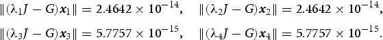Therefore, the system with J, G as coefficient matrices is of the eigenpairs $({\lambda }_i,{\mathit{x}}_i),i=1,2,3,4.$

Acknowledgements

The authors would like to express their heartfelt thanks to five anonymous reviewers for their constructive criticisms and helpful suggestions for the improvement of the quality of the paper.

Disclosure statement

No potential conflict of interest was reported by the authors.

References

- Meirovitch L. A modal analysis for the response of linear gyroscopic systems. ASME J Appl Mech. 1975;42:446–450.
- Meirovitch L. A new method of solution of the eigenvalue problem for gyroscopic systems. AIAA J. 1974;12:1337–1342.
- Yuan Y, Dai H. An inverse problem for undamped gyroscopic systems. J Comput Appl Math. 2012;236:2574–2581.
- Yuan Y, Guo Y. A direct updating method for damped gyroscopic systems using measured modal data. Appl Math Model. 2010;34:1450–1457.
- Mao X, Dai H. Structure preserving eigenvalue embedding for undamped gyroscopic systems. Appl Math Model. 2014;38:4333–4344.
- Lancaster P. Stability of linear gyroscopic systems: a review. Linear Algebra Appl. 2013;439:686–706.
- Ouyang H, Zhang J. Passive modifications for partial assignment of natural frequencies of mass-spring systems. Mech Syst Signal Process. 2015;50–51:214–226.
- Tresser S, Bucher I. Balancing fast flexible gyroscopic systems at low speed using parametric excitation. Mech Syst Signal Process. 2019;130:452–469.
- Cooley CG, Parker RG. Eigenvalue sensitivity and veering in gyroscopic systems with application to high-speed planetary gears. European J Mech – A/Solids. 2018;67:123–136.
- Lancaster P, Maroulas J. Inverse eigenvalue problems for damped vibrating systems. J Math Anal Appl. 1987;123:238–261.
- Lancaster P, Ye Q. Inverse spectral problems for linear and quadratic matrix pencils. Linear Algebra Appl. 1988;107:293–309.
- Starek L, Inman DJ, Kress A. A symmetric inverse vibration problem. ASME J Vib Acoust. 1992;114:564–568.
- Starek L, Inman DJ. A symmetric inverse vibration problem with over-damped modes. J Sound Vib. 1995;181:893–903.
- Starek L, Inman DJ. A symmetric inverse vibration problem for non-proportional underdamped system. ASME J Appl Mech. 1997;64:601–605.
- Starek L, Inman DJ. Design of nonproportional damped systems via symmetric positive inverse problems. ASME J Vib Acoust. 2004;126:212–219.
- Friswell MI, Inman DJ, Pilkey DF. The direct updating of damping and stiffness matrices. AIAA J. 1998;36:491–493.
- Kuo Y-C, Lin W-W, Xu S-F. New methods for finite element model updating problems. AIAA J. 2006;44:1310–1316.
- Chu D, Chu MT, Lin W-W. Quadratic model updating with symmetry, positive definiteness, and no spill-over. SIAM J Matrix Anal Appl. 2009;31:546–564.
- Yuan Y, Dai H. On a class of inverse quadratic eigenvalue problem. J Comput Appl Math. 2011;235:2662–2669.
- Yuan Y, Liu H. A gradient based iterative algorithm for solving structural dynamics model updating problems. Meccanica. 2013;48:2245–2253.
- Rogers GS. Matrix derivatives. New York: Marcel Dekker, Inc.; 1980. (Lecture Notes in Statistics; 2).
- Wei Y, Zhang N, Ng MK, et al. Tikhonov regularization for weighted total least squares problems. Appl Math Lett. 2007;20:82–87.
- Aubin JP. Applied functional analysis. John Wiley & Sons: New York; 1979.
- Bai Z-Z. On Hermitian and skew-Hermitian splitting iteration methods for continuous Sylvester equations. J Comput Math. 2011;29:185–198.
- Zhou R, Wang X, Zhou P. A modified HSS iteration method for solving the complex linear matrix equation AXB = C. J Comput Math. 2016;34:437–450.
- Wang X, Li Y, Dai L. On Hermitian and skew-Hermitian splitting iteration methods for the linear matrix equation AXB = C. Computers and Math Appl. 2013;65:657–664.
- Zhou R, Wang X, Tang X-B. Preconditioned positive-definite and skew-Hermitian splitting iteration methods for continuous Sylvester equations AX + XB = C. East Asian J Appl Math. 2017;7:55–69.
- Wang X, Li W-W, Mao L-Z. On positive-definite and skew-Hermitian splitting iteration methods for continuous Sylvester equation AX + XB = C. Comput Math Appl. 2013;66:2352–2361.
- Albert A. Condition for positive and nonnegative definite in terms of pseudoinverse. SIAM J Appl Math. 1969;17:434–440.