A blocking scheme for dimension-robust Gibbs sampling in large-scale image deblurring

ABSTRACT

Among the most significant challenges with using Markov chain Monte Carlo (MCMC) methods for sampling from the posterior distributions of Bayesian inverse problems is the rate at which the sampling becomes computationally intractable, as a function of the number of estimated parameters. In image deblurring, there are many MCMC algorithms in the literature, but few attempt reconstructions for images larger than $512\times 512$ pixels (${10}^5$ parameters). In quantitative X-ray radiography, used to diagnose dynamic materials experiments, the images can be much larger, leading to problems with millions of parameters. We address this issue and construct a Gibbs sampler via a blocking scheme that leads to a sparse and highly structured posterior precision matrix. The Gibbs sampler naturally exploits the special matrix structure during sampling, making it ‘dimension-robust’, so that its mixing properties are nearly independent of the image size, and generating one sample is computationally feasible. The dimension-robustness enables the characterization of posteriors for large-scale image deblurring problems on modest computational platforms. We demonstrate applicability of this approach by deblurring radiographs of size $4096\times 4096$ pixels (${10}^7$ parameters) taken at the Cygnus Dual Beam X-ray Radiography Facility at the U.S. Department of Energy's Nevada National Security Site.

Keywords:

• Deconvolution
• Markov chain Monte Carlo
• Gibbs sampling

AMS classifications:

• 15A29
• 65F22
• 65C05
• 65C60
• 94A08

1. Introduction

As opposed to most digital photography – where the goal is to produce pictures that look as good as possible – the primary goal of quantitative imaging is to compute features in images for use in quantitative scientific studies. For example, in digital X-ray radiography, it is common to pulse X-rays to penetrate a scene, to convert the non-attenuated X-rays into visible light for capture on a CCD camera, and to compute features such as object locations or material densities from the resulting images [1–4]. Image blur, caused in particular by the finite extent of the X-ray source (it's not a point source), optical aberrations introduced by the lens system, and conversion of X-ray photons to light that is digitally recorded by conversion onto a CCD, makes computing scene features challenging [5–7]. There is an extensive literature on using convolution as a forward model for image blur (see [8] and the references therein), and a great deal of work has been done to formulate image deblurring within Bayesian frameworks and to develop Markov chain Monte Carlo (MCMC) methods for numerically describing the corresponding posteriors by a set of samples, so that expected values with respect to the posterior can be approximated by averages over the samples [9–16].

Most of the MCMC methods in image deblurring are based on Metropolis-Hastings samplers, or Gibbs samplers, or a combination of the two. The large-scale nature of many image deblurring problems, caused by the large number of pixels, makes MCMC computationally difficult, but several methods have been developed to keep the computational requirements of MCMC manageable, in particular for linear inverse problems and image deblurring. Fast and scalable methods for sampling high-dimensional Gaussians can be constructed by using analogies of Gibbs samplers with linear solvers. Examples include samplers that use matrix splitting to accelerate convergence [12, 13, 17] or that use (preconditioned) Krylov subspace methods [18–20]. We add to this line of work and devise a blocking scheme for a Gibbs sampler that makes it a practical tool for large-scale image deblurring.

1.1. Blocking schemes in Gibbs sampling

A fundamental property of Gibbs sampling, which is important in high-dimensional sampling problems, can be illustrated by the following example of a distribution $p(\mathbf{x})$ over a three-component parameter vector $\mathbf{x}=[x_1,x_2,x_3]$. Specifically, the Gibbs sampler can use any of the following iterations to produce samples from $p(\mathbf{x})$: $\begin{array}{ccc}\mathrm{Iteration}(\mathrm{a})& \mathrm{Iteration}(\mathrm{b})& \mathrm{Iteration}(\mathrm{c})\\ x_1^k,x_2^k,x_3^k\sim p(x_1,x_2,x_3)& x_1^k,x_2^k\sim p(x_1,x_2|x_3^{k-1})& x_1^k\sim p(x_1|x_2^{k-1},x_3^{k-1})\\ & x_3^k\sim p(x_3|x_1^k,x_2^k)& x_2^k\sim p(x_2|x_1^k,x_3^{k-1})\\ & & x_3^k\sim p(x_3|x_1^k,x_2^k),\end{array}$where k is the Markov chain iterate, and $x_1^0$, $x_2^0$, $x_3^0$ are assumed given. That is to say that we can group $x_1$, $x_2$, $x_3$ together and sample directly from the target distribution (independence sampler, Iteration (a)), sample each of $x_1$, $x_2$, and $x_3$ separately from their respective conditional distributions in any order (represented by Iteration (c)), or sample any combination of two and one or one and two parameters (represented by Iteration (b)). The way the parameters are grouped together within a Gibbs sampler is called its blocking scheme, and, while different blocking schemes for a Gibbs sampler will always result in a Markov chain whose stationary distribution is the correct target (see [21, 22]), all blocking schemes are not created equal with respect to the computational efficiency of each step in the Gibbs iteration nor with respect to the convergence properties of the Markov chain [23, 24].

1.2. Motivation and main result

The goal of the work presented here is to create an MCMC sampler that can compute samples from the Gaussian posterior of a Bayesian-formulated image deblurring problem that arises in quantitative X-ray radiography. The main obstacle is the large dimension of the problem. For a radiograph with $4096\times 4096$ pixels, the dimension of the problem is ${4096}^2\approx 1.6\cdot {10}^7$, since each pixel is an unknown. For a high-dimensional problem, one should use a ‘dimension-robust’ algorithm, that satisfies that

1. the mixing properties of the Markov chain do not degrade with dimension;

2. the computational requirements for generating one sample must be feasible

(see [25] for the original source of the term ‘dimension-robustness’). Achieving dimension-robustness is not straightforward. Typical MCMC samplers, such as random walk Metropolis (RWM), Metropolis adjusted Langevin algorithm (MALA), or Hamiltonian MCMC (HMC), are not dimension robust, because their (optimal) step size decreases with dimension [26–28]. Gibbs iterations of type (c) are not dimension-robust because its mixing properties degrade with dimension (unless the problem is a collection of independent random variables). Gibbs iterations of type (a) are not dimension-robust because the computational requirements for generating one sample are large, even when the posterior is Gaussian [13].

We construct a Gibbs sampler of type (b), with a blocking scheme that groups parameters together strategically to achieve dimension-robustness. The blocking scheme is chosen to exploit local properties of 2D convolution (representing blur) and to lead to a sparse and highly structured posterior precision matrix. Essentially, the blocking scheme groups together only those pixels that are ‘close’ to each other, where closeness depends on the size of the convolution kernel and length scales in the prior (which are often small compared to the size of the kernel). Because the blocking scheme results in blocks of strongly correlated parameters, the Markov chain generated by the Gibbs sampler has good mixing properties, even when the number of pixels is large. Such good mixing of the chain in high dimensions is one of the key concepts for dimension-robustness. A second key idea is finding the balance between working with a small number of large blocks vs. a large number of small blocks, which is a competition between a small number of expensive Gibbs iterates vs. a large number of inexpensive iterates.

Taken together, our ideas result in a Gibbs sampler that is capable of drawing samples from Gaussian posterior distributions with more than ${10}^7$ parameters using relatively modest computational platforms. The robustness of the ideas presented here is demonstrated by deblurring radiographs taken at the Cygnus Dual Beam X-ray Radiography Facility at the U.S. Department of Energy's Nevada National Security Site, a system whose images are significantly larger than those that typically appear in the literature [12, 29–34].

2. Bayesian convolution model with data-driven boundary conditions

A standard one-dimensional model for discrete convolution of a vector $\mathbf{x}\in {\mathbb{R}}^{n_x}$ with kernel $\mathbf{a}\in {\mathbb{R}}^{n_a}$ is a vector $\mathbf{b}\in {\mathbb{R}}^{n_b}$ given by (1) $\left[\begin{array}{c}{b}_1\\ b_2\\ ⋮\\ b_{n_b}\end{array}\right]=\left[\begin{array}{ccccc}{a}_{n_a}& \dots & \dots & \dots & a_1\\ & a_{n_a}& \dots & \dots & \dots & a_1\\ & & \ddots & \ddots & \ddots & \ddots & \ddots \\ & & & a_{n_a}& \dots & \dots & \dots & a_1\\ & & & & a_{n_a}& \dots & \dots & \dots & a_1\end{array}\right]\left[\begin{array}{c}{x}_1\\ x_2\\ ⋮\\ ⋮\\ x_{n_x}\end{array}\right],$(1) and we denote the convolution matrix by $\mathbf{A}\in {\mathbb{R}}^{n_b\times n_x}$, where $n_x=n_b+n_a-1$.

In imaging applications, $\mathbf{b}$ is the measured, blurry image, $\mathbf{a}$ is the blur kernel (the so-called point spread function), and $\mathbf{x}$ is the ideal, or deblurred image. Despite (1(1) $\left[\begin{array}{c}{b}_1\\ b_2\\ ⋮\\ b_{n_b}\end{array}\right]=\left[\begin{array}{ccccc}{a}_{n_a}& \dots & \dots & \dots & a_1\\ & a_{n_a}& \dots & \dots & \dots & a_1\\ & & \ddots & \ddots & \ddots & \ddots & \ddots \\ & & & a_{n_a}& \dots & \dots & \dots & a_1\\ & & & & a_{n_a}& \dots & \dots & \dots & a_1\end{array}\right]\left[\begin{array}{c}{x}_1\\ x_2\\ ⋮\\ ⋮\\ x_{n_x}\end{array}\right],$(1) ) being a common model for image blur, it is actually somewhat unnatural in imaging applications, because it implies that the domain of the blury image $\mathbf{b}\in {\mathbb{R}}^{n_b}$, also called the ‘field of view ', is not the same as the domain of the ideal image $\mathbf{x}\in {\mathbb{R}}^{n_x}$. To fix that discrepancy, boundary conditions, like periodic, zero, or reflective, are often imposed to provide formulas for the parameters outside of the field of view, based on those within the field of view. This approach effectively shrinks the unknown $\mathbf{x}$ to have the same dimension as the blurry image ($n_x=n_b$). Thus, $\mathbf{A}$ is a square convolution matrix, and the linear system that defines $\mathbf{x}$ given $\mathbf{b}$ and $\mathbf{A}$ can be solved using computationally efficient methods. Standard boundary conditions, however, are also unnatural impositions in imaging applications, a picture taken of an experiment will never exist on a torus (as periodic boundaries imply) or be perfectly dark outside of the field of view (as zero boundaries imply).

Rather than shrink the problem to a smaller dimension, an alternate approach – introduced in [35, 36] and fully detailed in [10] – is to instead solve the larger problem of reconstructing the full vector $\mathbf{x}$ of size $n_x=n_b+n_a-1$. Assuming periodic boundary conditions on $\mathbf{x}$ and extending the point spread function by padding on the front and back with $(n_b-1)/2$¹ zeros gives $\hat{\mathbf{a}}=[0,\dots ,0,a_{n_a},\dots ,a_1,0,\dots ,0],$resulting in $\hat{\mathbf{a}}\in {\mathbb{R}}^{n_x}$ with a corresponding convolution matrix $\hat{\mathbf{A}}\in {\mathbb{R}}^{n_x\times n_x}$, taking into account periodic boundary conditions on this extended domain. Note that assuming periodic boundary conditions on this extended domain is no longer unnatural, since boundary artefacts can only impact the values of $\mathbf{x}$ outside of the field of view. Since the size of the data (the blurry image) is still $n_b$, we then define the matrix $\mathbf{D}\in {\mathbb{R}}^{n_b\times n_x}$ to have the middle $n_b$ rows of the identity of size $n_x\times n_x$. This matrix has the effect of picking out the centre $n_b$ elements of a vector of length $n_x$ so that $\mathbf{b}=\mathbf{D}\hat{\mathbf{A}}\mathbf{x}$. Throughout the remainder of this work, these ‘data-driven’ boundary conditions are applied. It is straightforward to extend these ideas to two dimensions (actual images). In 2D, we denote the number of rows of pixels of an image by m and the number of columns of pixel by n (often with sub-indices, see Table A1 for details). The blurring kernel, $\mathbf{a}$, is also a two-dimensional object with $m_a$ rows and $n_a$ columns. This leads to a convolution matrix, $\mathbf{A}$, with $m_x$ rows and $n_x$ columns, where $m_x$ and $n_x$ are the number of rows and columns of the reconstructed image.

A Bayesian formulation of the deblurring problem requires that we model errors by random variables. Here, we use a simple (but popular) additive Gaussian error model and write (2) $\mathbf{b}=\mathbf{A}\mathbf{x}+\mathit{\epsilon },$(2) where $\mathit{\epsilon }\sim \mathcal{N}(\mathbf{0},{\lambda }^{-1}\mathbf{I})$ with precision parameter $\lambda >0$ and, throughout the paper, $\mathcal{N}(\mathbf{y},\mathbf{\Sigma })$ denotes a Gaussian with mean $\mathbf{y}$ and covariance matrix $\mathbf{\Sigma }$. We further simplify the notation and write $\mathbf{A}$ for $\mathbf{D}\hat{\mathbf{A}}$, because we exclusively work with data-driven boundary conditions. Equation (2(2) $\mathbf{b}=\mathbf{A}\mathbf{x}+\mathit{\epsilon },$(2) ) defines the likelihood (3) $p(\mathbf{b}|\mathbf{x},\lambda )\propto \exp (-\frac{\lambda }{2}{\Vert \mathbf{A}\mathbf{x}-\mathbf{b}\Vert }^2),$(3) where $\Vert \cdot \Vert$ is the Euclidean norm, i.e. $\Vert \mathbf{y}\Vert =\sqrt{y_1^2+\cdots +y_{n_y}^2}$. To complete the Bayesian problem formulation, we define a Gaussian Markov random field prior [37, 38] by (4) $p(\mathbf{x}|\delta )\propto \exp (-\frac{\delta }{2}{\Vert {\mathbf{L}}^{1/2}\mathbf{x}\Vert }^2),$(4) where $\mathbf{L}$ is the discrete Laplacian operator, ${\mathbf{L}}^{1/2}$ is a matrix square root, and $\delta >0$ is a scalar. While we focus on using the Laplacian, other choices are also possible and easy to incorporate into our overall approach.

The posterior distribution is proportional to the product of the prior and the likelihood, (5) $p(\mathbf{x}|\mathbf{b},\lambda ,\delta )\propto \exp (-\frac{\lambda }{2}{\Vert \mathbf{A}\mathbf{x}-\mathbf{b}\Vert }^2-\frac{\delta }{2}{\Vert {\mathbf{L}}^{1/2}\mathbf{x}\Vert }^2).$(5) The goal is thus to draw samples from the Gaussian posterior distribution (5(5) $p(\mathbf{x}|\mathbf{b},\lambda ,\delta )\propto \exp (-\frac{\lambda }{2}{\Vert \mathbf{A}\mathbf{x}-\mathbf{b}\Vert }^2-\frac{\delta }{2}{\Vert {\mathbf{L}}^{1/2}\mathbf{x}\Vert }^2).$(5) ), $\mathbf{x}|\mathbf{b},\lambda ,\delta \sim \mathcal{N}(\mathbf{m},{\mathbf{H}}^{-1})$, with the posterior precision and mean (6) $\begin{array}{rl}& \mathbf{H}=\lambda {\mathbf{A}}^{\mathrm{\top }}\mathbf{A}+\delta \mathbf{L},\end{array}$(6) (7) $\begin{array}{rl}& \mathbf{m}=\lambda {\mathbf{H}}^{-1}{\mathbf{A}}^{\mathrm{\top }}\mathbf{b}.\end{array}$(7) Note that we assume the precision parameters λ and δ are given. It is also possible to use the Bayesian framework to estimate these parameters on the fly, via hierarchical models as in [37], but that is not done here.

2.1. Notation

We denote vectors by lower case bold face and matrices by upper case bold face and use n and m to denote dimensions. We stack the columns of pixels for an image as follows: for an image $\mathbf{Y}$ of size $m_y\times n_y$, the corresponding column stack vector is $\mathbf{y}\in {\mathbb{R}}^{m_y{n}_y\times 1}$. The proposed Gibbs sampler is notationally intensive, so a list of frequently used matrices, vectors, and sizes is included in Appendix (Table A1).

3. Gibbs sampling for large-scale image deblurring

Applying a Gibbs sampler in large-scale image deblurring at a reasonable computational cost requires that

1. a single sample can be generated in a short time, even if the image size is large;

2. the mixing properties of the Markov chain, generated by the sampler, do not degrade catastrophically with the size of the image.

In this section, we describe how to construct and implement a sub-image based blocking scheme that leads to a Gibbs sampler that satisfies both of the above requirements. We start with a brief review of the basics of Gibbs sampling in Section 3.1, then describe the sub-image based blocking scheme in Section 3.2. This blocking scheme is constructed to exploit the local nature of convolution and regularization to result in well-structured and sparse convolution, prior precision, and posterior precision matrices. Exploiting this special matrix structure within the 2D environment characteristic of imaging problems is key for the applicability of the sampler in large-scale problems.

Section 3.3 details how the size of the sub-images needs to be chosen to balance the effort required to compute a single sample in the Markov chain with the mixing properties of the Markov chain, i.e. how many samples in the chain are required to characterize the posterior. Section 3.4 discusses why it is expected that Gibbs samplers, with the sub-image based blocking scheme, are ‘dimension-robust ', which is to say that their mixing properties depend only mildly on the size of the image. Section 3.5 provides details of the implementation of the sampler. The images in our target application in X-ray radiography have $16\cdot {10}^6$ pixels, which results in posterior precision matrices of size $(16\cdot {10}^6)\times (16\cdot {10}^6)$. Assembly of such large matrices is prohibitively expensive, even if we exploit their sparsity, so a matrix-free implementation of the sampler is described.

3.1. Review of Gibbs sampling

The basic idea of a Gibbs sampler in the context of drawing samples from an $n_x$-dimensional Gaussian (posterior) distribution $\mathbf{x}\sim \mathcal{N}(\mathbf{m},{\mathbf{H}}^{-1})$ is to partition $\mathbf{x}$ into $n_p$ blocks, (8) $\mathbf{x}=[{\mathbf{x}}_1,\dots ,{\mathbf{x}}_{n_p}],$(8) where each ${\mathbf{x}}_i$ is an $n_d=n_x/n_p$ dimensional vector, and to subsequently use the conditional distributions (9) $p({\mathbf{x}}_i|{\mathbf{x}}_1,\dots ,{\mathbf{x}}_{i-1},{\mathbf{x}}_{i+1},\dots {\mathbf{x}}_{n_p}),$(9) for sampling [21, 38–40]. For a Gaussian posterior, the conditional distributions are also Gaussians, (10) ${\mathbf{x}}_i|{\mathbf{x}}_1,\dots ,{\mathbf{x}}_{i-1},{\mathbf{x}}_{i+1},\dots {\mathbf{x}}_{n_p}\sim \mathcal{N}({\mathbf{m}}_i-\sum _{j\ne i}{\mathbf{H}}_{ij}({\mathbf{x}}_j-{\mathbf{m}}_j),{\mathbf{H}}_{ii}^{-1}),$(10) where ${\mathbf{H}}_{ij}$, $i,j=1,\dots ,n_p$ are $n_d\times n_d$ dimensional sub-matrices of the posterior precision matrix $\mathbf{H}$ and ${\mathbf{m}}_i$ are blocks of the posterior mean $\mathbf{m}$. Given a sample ${\mathbf{x}}^{k-1}$, the Gibbs sampler generates a new sample ${\mathbf{x}}^k$, by cycling through the $n_p$ blocks and sampling the conditional distributions (11) ${\mathbf{x}}_i^k\sim \mathcal{N}({\mathbf{m}}_i-(\sum _{j>i}{\mathbf{H}}_{ij}({\mathbf{x}}_j^{k-1}-{\mathbf{m}}_j)+\sum _{j<i}{\mathbf{H}}_{ij}({\mathbf{x}}_j^k-{\mathbf{m}}_j)),{\mathbf{H}}_{ii}^{-1}).$(11) Note that subscript denotes the block index and superscript denotes the iteration number in the Markov chain. Thus, the Gibbs sampler uses the current iterate ${\mathbf{x}}^k$ for blocks that have already been sampled in the current cycle and the previous iterate, ${\mathbf{x}}^{k-1}$, for blocks that have not yet been updated. The full Gibbs sampler is summarized in Algorithm 1.

3.2. Efficient blocking via sub-images

How the image $\mathbf{X}$ is vectorized is arbitrary in theory, but important in practice, because it defines the structure of the blurring matrix $\mathbf{A}$, the prior precision $\mathbf{L}$ and, thus, the posterior precision $\mathbf{H}$. For example, the Laplacian $\mathbf{L}$ is sparse for any method of constructing $\mathbf{x}$ from $\mathbf{X}$, but it is banded if $\mathbf{x}$ is a column stack. Thus the way the vector $\mathbf{x}$ is defined from the image $\mathbf{X}$ determines the sparsity patterns of the matrices $\mathbf{A}$, $\mathbf{L}$, and $\mathbf{H}$. The sparsity pattern of $\mathbf{H}$ is important for the Gibbs sampler, because $\mathbf{H}$ encodes conditional independencies among the blocks, which in turn defines the mixing properties of the Markov chain [23, 24].

Rather than using the column stack, we define the vector $\mathbf{x}$ based on column stacks of sub-images. Specifically, we partition the image $\mathbf{X}$ into a set of $n_p=m_B\cdot n_B$ sub-images ${\mathbf{X}}_i$, each of size $m_d\times n_d$, (12) $\mathbf{X}=\left[\begin{array}{cccc}{\mathbf{X}}_1& {\mathbf{X}}_{1+m_B}& \cdots & {\mathbf{X}}_{1+m_B(n_B-1)}\\ {\mathbf{X}}_2& {\mathbf{X}}_{2+m_B}& \cdots & {\mathbf{X}}_{2+m_B(n_B-1)}\\ ⋮& ⋮& \ddots & ⋮\\ {\mathbf{X}}_{m_B}& {\mathbf{X}}_{2m_B}& \cdots & {\mathbf{X}}_{m_B{n}_B}\end{array}\right].$(12) The N-dimensional vector $\mathbf{x}$ is now formed by column stacks of the sub-images. It is assumed that the sub-images are of equal size and that they are indexed top to bottom, left to right, but neither is critical.

To see why a blocking based on sub-images is advantageous in Gibbs sampling, recall that blurring and the Laplacian prior precision define ‘local’ actions – only pixels that are spatially nearby are blurred or used for computing derivatives. The posterior precision matrix $\mathbf{H}$ is defined in terms of the blurring and prior precision matrix (see (6(6) $\begin{array}{rl}& \mathbf{H}=\lambda {\mathbf{A}}^{\mathrm{\top }}\mathbf{A}+\delta \mathbf{L},\end{array}$(6) )) and, thus also defines local actions. Because a precision matrix encodes conditional independencies, the local nature of $\mathbf{H}$ implies that far-away sub-images are conditionally independent. Since we define the blocks of $\mathbf{x}$ by column stacks of the sub-images, this implies that ${\mathbf{x}}_j$ is conditionally independent of most other blocks.

3.2.1. Illustration of the sub-image based blocking scheme

The sub-image based blocking scheme can be illustrated by an example of a $100\times 100$ image $\mathbf{X}$, blurred by a kernel size of size $21\times 21$. We partition the image into $m_B\times n_B=10\times 10$ sub-images, each of size $m_d\times n_d=10\times 10$. Because the sub-image size is greater than half the kernel size minus one ($10>9.5=21/2-1$), each sub-image conditionally depends on only eight surrounding sub-images. This means that the sums in the Gibbs sampler (see (11(11) ${\mathbf{x}}_i^k\sim \mathcal{N}({\mathbf{m}}_i-(\sum _{j>i}{\mathbf{H}}_{ij}({\mathbf{x}}_j^{k-1}-{\mathbf{m}}_j)+\sum _{j<i}{\mathbf{H}}_{ij}({\mathbf{x}}_j^k-{\mathbf{m}}_j)),{\mathbf{H}}_{ii}^{-1}).$(11) )) extend over blocks ${\mathbf{x}}_j$, corresponding to these eight sub-images only, as is illustrated in Figure 1(a).Here, the yellow sub-image corresponds to the block ${\mathbf{x}}_i^k$ that is currently being updated by the Gibbs sampler during the $k^{\mathrm{th}}$ iteration. By our construction, ${\mathbf{x}}_i^k$ conditionally depends only on the eight neighbouring sub-images highlighted in blue and green, but is conditionally independent of the 91 remaining sub-images. Assuming the indexing in (12(12) $\mathbf{X}=\left[\begin{array}{cccc}{\mathbf{X}}_1& {\mathbf{X}}_{1+m_B}& \cdots & {\mathbf{X}}_{1+m_B(n_B-1)}\\ {\mathbf{X}}_2& {\mathbf{X}}_{2+m_B}& \cdots & {\mathbf{X}}_{2+m_B(n_B-1)}\\ ⋮& ⋮& \ddots & ⋮\\ {\mathbf{X}}_{m_B}& {\mathbf{X}}_{2m_B}& \cdots & {\mathbf{X}}_{m_B{n}_B}\end{array}\right].$(12) ), the Gibbs sampler cycles from top to bottom, left to right. Thus, the four blue sub-images correspond to blocks that have already been updated during iteration k; the four green sub-images have not been updated during iteration k.

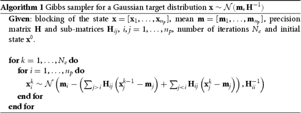
Figure 1. Illustration of the sub-image based blocking scheme and comparison with column stack based blocking. Shown is the domain of a $100\times 100$ image, blurred by a kernel of size $21\times 21$. In panel (a), a block is defined by a column stack of a sub-image. The sub-image corresponding to the block that is currently being updated is highlighted in yellow; this block is conditionally independent of the 91 sub-images whose domains are shown in white, but is conditionally dependent on the eight sub-images highlighted in blue and green. In panel (b), a block is defined by a column of the image. The block, currently being updated, is highlighted in yellow; this block is conditionally independent of the 79 blocks shown in white, but is conditionally dependent on 20 other blocks, highlighted in blue and green. (a) Sub-image based blocking scheme, (b) column stack based blocking scheme.

We compare the sub-image based blocking scheme with the more common blocking that results from generating the vector $\mathbf{x}$ by a column stack of the entire image $\mathbf{X}$. In this case, the block ${\mathbf{x}}_i$, which is a column of the image $\mathbf{X}$, depends conditionally on ten blocks to the left and ten blocks to the right (due to the kernel size of $21\times 21$). This is illustrated in Figure 1(b), where ${\mathbf{x}}_i$ is highlighted in yellow and where the conditionally dependent blocks are highlighted in blue and green. Assuming that we generate $\mathbf{x}$ by column-stacking the columns of $\mathbf{X}$ left to right, the Gibbs sampler has visited the blue blocks to the left of ${\mathbf{x}}_i$, but has not yet visited the green blocks to the right.

In summary, the blocking scheme based on sub-images requires conditioning each block on only eight nearby blocks of 100 pixels each (800 pixels in total). A blocking scheme based on a column stack of the image requires conditioning each block on 20 neighbouring blocks, each consisting of 100 pixels (2000 pixels in total).

3.3. Optimal and practical sub-image size

The sub-image based blocking scheme offers flexibility in the size of the sub-images in that any sub-image size will lead to a Gibbs sampler that asymptotically (large sample limit) samples the target distribution. Nonetheless, some sub-image sizes may lead to more efficient samplers than others. A practically relevant sub-image size must resolve a trade-off characteristic of many MCMC schemes, that the computations required for computing a single sample in the Markov chain must be balanced with the overall mixing properties of the chain. For example, using the entire image as the single ‘sub-image’, the Gibbs sampler described above amounts to drawing independent samples from the Gaussian posterior distribution (perfect mixing of the chain). For large images, generating samples in this way becomes impractical (large cost per sample). On the other extreme, using a single pixel as a sub-image requires only scalar operations (small cost per sample), but there are large correlations in consecutive steps of the chain (slow mixing of the chain).

An optimal choice of the sub-image size would balance the cost-per-sample with the overall mixing properties of the chain. Such an optimal sub-image size is difficult to anticipate and to describe in generality, because it is problem dependent. Specifically, it is a function of the ratio of the kernel size to the overall image size and the computer used to run the computations. For example, it is not needed to use the proposed Gibbs sampler for images of size $1024\times 1024$ or less. Given today's typical desktop's or even laptop's computing power, one can draw direct samples (independence sampler, see Iteration (a) in Section 1) for such ‘small’ images.

The Gibbs sampler described above provides the greatest advantages for large images, blurred by large kernels. In this case, the sub-images should be chosen larger than half of the kernel size, so that (13) $m_d\ge \frac{m_a-1}{2},n_d\ge \frac{n_a-1}{2}.$(13) With sub-images of this size (or larger) each block conditionally depends on only eight neighbouring blocks (see also the illustrative example above). The numerical experiments in Section 4 suggest that the sub-image size is not critical for the mixing properties of the chain (as long as (13(13) $m_d\ge \frac{m_a-1}{2},n_d\ge \frac{n_a-1}{2}.$(13) ) is satisfied). We thus define the ‘practical’ sub-image size as the sub-image size that satisfies (13(13) $m_d\ge \frac{m_a-1}{2},n_d\ge \frac{n_a-1}{2}.$(13) ) and minimizes the computation time for generating one sample.

3.4. Dimension-robustness

The goal is to use the Gibbs sampler for large-scale image deblurring, which requires that its mixing properties do not degrade with dimension or, equivalently, image size. This issue was discussed, in a more general setting, in [23], where it was shown that the convergence rate of a Gibbs sampler for Gaussians with block tridiagonal covariance or precision matrices is independent of the dimension of the Gaussian. The dimension independent convergence rate makes the Gibbs sampler a suitable algorithm for high-dimensional problems. The block tridiagonal structure, assumed in [23], indeed occurs naturally in the 1-dimensional model for discrete convolution (see Section 1). Thus, a Gibbs sampler has a dimension independent convergence rate when applied to 1D deblurring problems, but the 2D nature of image deblurring violates the assumption of a block tridiagonal precision matrix. Thus, previous results about dimension independent convergence rates cannot be directly transferred to our case of interest.

We do not attempt to extend the proof in [23] to a 2D image deblurring problem, but rather demonstrate numerically that the mixing properties of the Gibbs sampler, with a carefully defined sub-image size, do not degrade with dimension. In the language of [25], we thus show that the algorithm is ‘dimension-robust '. The fact that we have no formal proof of dimension independence can be interpreted as another instance of ‘bad theory for good algorithms’, as reported in [25], where the case is made for practical, high-dimensional sampling algorithms being intrinsically difficult to analyse rigorously.

3.5. Matrix-based and matrix-free implementations

Recall that the sub-image based blocking scheme means that $\mathbf{x}$ and its blocks ${\mathbf{x}}_i$, $i=1,\dots ,n_p$, are defined by column stacks of the sub-images ${\mathbf{X}}_i$. This construction of $\mathbf{x}$ determines the construction of the blurring matrix $\mathbf{A}$ and the prior precision matrix $\mathbf{L}$, which in turn determine the posterior precision matrix $\mathbf{H}$ and its sub-matrices ${\mathbf{H}}_{ij}$, $i,j=1,\dots ,n_p$. Given the matrices $\mathbf{A}$ and $\mathbf{L}$ – and thus $\mathbf{H}$ (see equation (6(6) $\begin{array}{rl}& \mathbf{H}=\lambda {\mathbf{A}}^{\mathrm{\top }}\mathbf{A}+\delta \mathbf{L},\end{array}$(6) )) – the posterior mean can be computed by solving (14) $\mathbf{H}\mathbf{m}=\lambda {\mathbf{A}}^{\mathrm{\top }}\mathbf{b},$(14) for $\mathbf{m}$, e.g. by using the conjugate gradient (CG) method. The definition of $\mathbf{x}$ via sub-images thus also defines the blocks of the mean $\mathbf{m}=[{\mathbf{m}}_1,\dots ,{\mathbf{m}}_{n_p}]$. Assuming that the sub-images are large enough so that (13(13) $m_d\ge \frac{m_a-1}{2},n_d\ge \frac{n_a-1}{2}.$(13) ) is satisfied, the update equation for the $i^{\mathrm{th}}$ block (see (11(11) ${\mathbf{x}}_i^k\sim \mathcal{N}({\mathbf{m}}_i-(\sum _{j>i}{\mathbf{H}}_{ij}({\mathbf{x}}_j^{k-1}-{\mathbf{m}}_j)+\sum _{j<i}{\mathbf{H}}_{ij}({\mathbf{x}}_j^k-{\mathbf{m}}_j)),{\mathbf{H}}_{ii}^{-1}).$(11) )) becomes (15) ${\mathbf{x}}_i^k\sim \mathcal{N}({\mathbf{m}}_i-(\sum _{j\in {\mathcal{S}}_{\mathrm{post}}}{\mathbf{H}}_{ij}({\mathbf{x}}_j^{k-1}-{\mathbf{m}}_j)+\sum _{j\in {\mathcal{S}}_{\mathrm{pre}}}{\mathbf{H}}_{ij}({\mathbf{x}}_j^k-{\mathbf{m}}_j)),{\mathbf{H}}_{ii}^{-1}),$(15) where the index sets (16) $\begin{array}{rl}{\mathcal{S}}_{\mathrm{pre}}& =\{i-m_B-1,i-m_B,i-m_B+1,i-1\}\cap \{1,\dots ,n_p\}\end{array}$(16) (17) $\begin{array}{rl}{\mathcal{S}}_{\mathrm{post}}& =\{i+1,i+m_B-1,i+m_B,i+m_B+1\}\cap \{1,\dots ,n_p\}.\end{array}$(17) define the blocks corresponding to the eight neighbouring sub-images. Here, ${\mathcal{S}}_{\mathrm{pre}}$ refers to sub-images that have already been updated during iteration k, and ${\mathcal{S}}_{\mathrm{post}}$ refers to sub-images that have not been updated in iteration k. We can implement drawing samples from this Gaussian by (18) ${\mathbf{x}}_i^k={\mathbf{m}}_i+{\mathbf{H}}_{ii}^{-1}[{\mathbf{H}}_{ii}^{\mathrm{\top }/2}\mathbf{z}-(\sum _{j\in {\mathcal{S}}_{\mathrm{post}}}{\mathbf{H}}_{ij}({\mathbf{x}}_j^{k-1}-{\mathbf{m}}_j)+\sum _{j\in {\mathcal{S}}_{\mathrm{pre}}}{\mathbf{H}}_{ij}({\mathbf{x}}_j^k-{\mathbf{m}}_j))],$(18) where $\mathbf{z}\sim \mathcal{N}(\mathbf{0},\mathbf{I})$. For small images, one can construct $\mathbf{A}$, $\mathbf{L}$ and $\mathbf{H}$ and compute ${\mathbf{x}}_i^k$ via (18(18) ${\mathbf{x}}_i^k={\mathbf{m}}_i+{\mathbf{H}}_{ii}^{-1}[{\mathbf{H}}_{ii}^{\mathrm{\top }/2}\mathbf{z}-(\sum _{j\in {\mathcal{S}}_{\mathrm{post}}}{\mathbf{H}}_{ij}({\mathbf{x}}_j^{k-1}-{\mathbf{m}}_j)+\sum _{j\in {\mathcal{S}}_{\mathrm{pre}}}{\mathbf{H}}_{ij}({\mathbf{x}}_j^k-{\mathbf{m}}_j))],$(18) ), implementing the inversion of ${\mathbf{H}}_{ii}$ by CG or similar algorithms.

For large images, constructing the posterior precision matrix $\mathbf{H}$ or its sub-matrices ${\mathbf{H}}_{ij}$ can be cumbersome and memory intensive. Instead of explicitly building the sub-matrices, we briefly describe how to exploit structure in the operators $\mathbf{A}$ and $\mathbf{L}$ to construct functions that perform the actions of the sub-matrices ${\mathbf{H}}_{ij}$ on sub-images, without assembling $\mathbf{H}$ or its sub-matrices ${\mathbf{H}}_{ij}$.

There are three separate computational elements in (18(18) ${\mathbf{x}}_i^k={\mathbf{m}}_i+{\mathbf{H}}_{ii}^{-1}[{\mathbf{H}}_{ii}^{\mathrm{\top }/2}\mathbf{z}-(\sum _{j\in {\mathcal{S}}_{\mathrm{post}}}{\mathbf{H}}_{ij}({\mathbf{x}}_j^{k-1}-{\mathbf{m}}_j)+\sum _{j\in {\mathcal{S}}_{\mathrm{pre}}}{\mathbf{H}}_{ij}({\mathbf{x}}_j^k-{\mathbf{m}}_j))],$(18) ), for which matrix-free implementations should be used:

1. Performing a back-solve to compute the action of the inverse of the sub-matrices ${\mathbf{H}}_{ii}$, i.e. build a function such that (19) $f_{\mathrm{diag}}(\mathbf{y},i)={\mathbf{H}}_{ii}^{-1}\mathbf{y}.$(19)

2. Compute the pre- and post-sums, i.e. build functions such that (20) $f_{\mathrm{pre}}(\mathbf{y},i)=\sum _{j\in {\mathcal{S}}_{\mathrm{pre}}}{\mathbf{H}}_{ij}{\mathbf{y}}_j\mathrm{and}{f}_{\mathrm{post}}(\mathbf{y},i)=\sum _{j\in {\mathcal{S}}_{\mathrm{post}}}{\mathbf{H}}_{ij}{\mathbf{y}}_j.$(20)

3. Generate a vector distributed as $\mathcal{N}(\mathbf{0},{\mathbf{H}}_{ii})$.

Each of these functions requires a representation of the action of sub-matrices ${\mathbf{H}}_{ij}$, which are defined by the blurring matrix $\mathbf{A}$ and the prior precision $\mathbf{L}$ (see (6(6) $\begin{array}{rl}& \mathbf{H}=\lambda {\mathbf{A}}^{\mathrm{\top }}\mathbf{A}+\delta \mathbf{L},\end{array}$(6) )). Given the sub-image blocking scheme $\mathbf{x}=[{\mathbf{x}}_1,\dots ,{\mathbf{x}}_{n_p}]$, the matrices $\mathbf{A}$ and $\mathbf{L}$ consist of $n_p\times n_p$ blocks, each of size $m_d{n}_d\times m_d{n}_d$. The sub-matrices ${\mathbf{H}}_{ij}$ thus can be expressed in terms of sub-matrices of $\mathbf{A}$ and $\mathbf{L}$: (21) ${\mathbf{H}}_{ij}=\lambda {\left({\mathbf{A}}_{:,i}\right)}^{\mathrm{\top }}{\mathbf{A}}_{:,j}+\delta {\mathbf{L}}_{ij}$(21) where (22) ${\mathbf{A}}_{:,j}={[{\mathbf{A}}_{1,j}^{\mathrm{\top }}\cdots {\mathbf{A}}_{n_p,j}^{\mathrm{\top }}]}^{\mathrm{\top }}.$(22) An implementation of the action of ${\mathbf{H}}_{ij}$ thus requires that we define the functions (23) $\begin{array}{rl}{f}_{{\mathbf{A}}_{:,j}}(\mathbf{y})& ={\mathbf{A}}_{:,j}\mathbf{y},\end{array}$(23) (24) $\begin{array}{rl}{f}_{({\mathbf{A}}_{:,i}{)}^{\mathrm{\top }}}(\mathbf{y})& =({\mathbf{A}}_{:,i}{)}^{\mathrm{\top }}\mathbf{y},\end{array}$(24) (25) $\begin{array}{rl}{f}_{{\mathbf{L}}_{ij}}(\mathbf{y})& ={\mathbf{L}}_{ij}\mathbf{y}.\end{array}$(25) We provide a brief summary of how to construct these functions here, with more details in the appendix. We refer to [41] for a description of all delicate details, especially with respect to a careful treatment of the data-driven boundary conditions.

In short, the function (23(23) $\begin{array}{rl}{f}_{{\mathbf{A}}_{:,j}}(\mathbf{y})& ={\mathbf{A}}_{:,j}\mathbf{y},\end{array}$(23) ) is equivalent to the action of the convolution matrix $\mathbf{A}$ acting on an image in which only the jth block is nonzero and equal to ${\mathbf{x}}_j$. It is possible to compute just the convolution with the non-zero portion of the image so that $f_{{\mathbf{A}}_{:,j}}(\cdot )$ can be implemented by convolving a small image with a given kernel via FFT. The function $f_{({\mathbf{A}}_{:,i}{)}^{\mathrm{\top }}}(\mathbf{y})$ in (24(24) $\begin{array}{rl}{f}_{({\mathbf{A}}_{:,i}{)}^{\mathrm{\top }}}(\mathbf{y})& =({\mathbf{A}}_{:,i}{)}^{\mathrm{\top }}\mathbf{y},\end{array}$(24) ) can be implemented in the same way, because the transpose essentially amounts to flipping the blurring kernel in the vertical and horizontal dimensions. The function $f_{{\mathbf{L}}_{ij}}(\mathbf{y})$ in (25(25) $\begin{array}{rl}{f}_{{\mathbf{L}}_{ij}}(\mathbf{y})& ={\mathbf{L}}_{ij}\mathbf{y}.\end{array}$(25) ) implements the action of sub-matrices of the negative 2D Laplacian, which is equivalent to convolution with the kernel $\left[\begin{array}{ccc}0& -1& 0\\ -1& 4& -1\\ 0& -1& 0\end{array}\right].$We can thus use the same ideas as above to implement (25(25) $\begin{array}{rl}{f}_{{\mathbf{L}}_{ij}}(\mathbf{y})& ={\mathbf{L}}_{ij}\mathbf{y}.\end{array}$(25) ).

Given the functions (23(23) $\begin{array}{rl}{f}_{{\mathbf{A}}_{:,j}}(\mathbf{y})& ={\mathbf{A}}_{:,j}\mathbf{y},\end{array}$(23) )–(25(25) $\begin{array}{rl}{f}_{{\mathbf{L}}_{ij}}(\mathbf{y})& ={\mathbf{L}}_{ij}\mathbf{y}.\end{array}$(25) ), the action of a sub-matrix ${\mathbf{H}}_{ii}$ on a vector ${\mathbf{x}}_i$ can be written as (26) $f_{{\mathbf{H}}_{ii}}({\mathbf{x}}_i)=\lambda f_{({\mathbf{A}}_{:,i}{)}^{\mathrm{\top }}}\left(f_{{\mathbf{A}}_{:,i}}\left({\mathbf{x}}_i\right)\right)+\delta f_{{\mathbf{L}}_{ii}}({\mathbf{x}}_i),$(26) and, given (26(26) $f_{{\mathbf{H}}_{ii}}({\mathbf{x}}_i)=\lambda f_{({\mathbf{A}}_{:,i}{)}^{\mathrm{\top }}}\left(f_{{\mathbf{A}}_{:,i}}\left({\mathbf{x}}_i\right)\right)+\delta f_{{\mathbf{L}}_{ii}}({\mathbf{x}}_i),$(26) ), we use CG to compute (19(19) $f_{\mathrm{diag}}(\mathbf{y},i)={\mathbf{H}}_{ii}^{-1}\mathbf{y}.$(19) ). To draw samples $\mathbf{v}\sim \mathcal{N}(\mathbf{0},{\mathbf{H}}_{ii})$, note that $\mathbf{v}={\mathbf{v}}_1+{\mathbf{v}}_2$, where ${\mathbf{v}}_1\sim \mathcal{N}(\mathbf{0},\lambda {\mathbf{A}}_{:,i}^{\mathrm{\top }}{\mathbf{A}}_{:,i})$ and ${\mathbf{v}}_2\sim \mathcal{N}(\mathbf{0},\delta {\mathbf{L}}_{ii})$ are two independent Gaussians. We can sample ${\mathbf{v}}_1$ by using the function $f_{({\mathbf{A}}_{:,i}{)}^{\mathrm{\top }}}(\cdot )$ and writing ${\mathbf{v}}_2=f_{({\mathbf{A}}_{:,i}{)}^{\mathrm{\top }}}(\mathbf{z})$, where $\mathbf{z}\sim \mathcal{N}(\mathbf{0},\mathbf{I})$; ${\mathbf{v}}_2$ can be sampled similarly (see Appendix). Similarly, the pre- and post-sums in (20(20) $f_{\mathrm{pre}}(\mathbf{y},i)=\sum _{j\in {\mathcal{S}}_{\mathrm{pre}}}{\mathbf{H}}_{ij}{\mathbf{y}}_j\mathrm{and}{f}_{\mathrm{post}}(\mathbf{y},i)=\sum _{j\in {\mathcal{S}}_{\mathrm{post}}}{\mathbf{H}}_{ij}{\mathbf{y}}_j.$(20) ) can be computed by $f_{({\mathbf{A}}_{:,i}{)}^{\mathrm{\top }}}(\cdot )$, convolution with a kernel, and slight modifications of the function $f_{{\mathbf{L}}_{ii}}(\cdot )$. The key idea here is to carefully construct sub-images that are used by these functions in the computation of the pre- and post-sums.

Note that the Gibbs sampler (in matrix-based or matrix free implementation), requires that we compute the posterior mean before we start sampling. This means that we need to solve (14(14) $\mathbf{H}\mathbf{m}=\lambda {\mathbf{A}}^{\mathrm{\top }}\mathbf{b},$(14) ) once, before we start the sampler. This is done by using CG and the functions implementing the action of $\mathbf{H}$ in the matrix-free implementation, or by simply solving (7(7) $\begin{array}{rl}& \mathbf{m}=\lambda {\mathbf{H}}^{-1}{\mathbf{A}}^{\mathrm{\top }}\mathbf{b}.\end{array}$(7) ), with given $\mathbf{H}$, in the matrix-based implementation.

Finally, we emphasize again that the Gibbs sampler should only be used for large images (larger than $1024\times 1024$ pixels), because smaller images can be dealt with by drawing samples directly from the Gaussian defined by Equations (6(6) $\begin{array}{rl}& \mathbf{H}=\lambda {\mathbf{A}}^{\mathrm{\top }}\mathbf{A}+\delta \mathbf{L},\end{array}$(6) )–(7(7) $\begin{array}{rl}& \mathbf{m}=\lambda {\mathbf{H}}^{-1}{\mathbf{A}}^{\mathrm{\top }}\mathbf{b}.\end{array}$(7) ). Thus, the matrix-based implementation we describe should be viewed as a conceptual tool to understand how the sampler works, rather than a practical algorithm.

4. Applications to X-ray radiography

Within the U.S. Department of Energy's research and development enterprise, X-ray radiography is a common approach to diagnosing dynamic material studies, where in situ measurements systems would be destroyed. One such facility is the Cygnus Dual Axis X-ray system at the Nevada National Security Site. One of the primary applications for such imaging is to understand the evolution of material density during shock compression, which can be modelled as a single-projection tomography for objects that are radially symmetric [3, 42, 43]. This requires sufficiently high spatial resolution, or more specifically, the ability to precisely measure distances in the imaging plane to the object's axis of symmetry and a complete understanding of the X-ray spectrum and fluence, which is necessary to convert from units of pixel intensity to areal density (g/cm${}^2$) [44–46]. Both of these aspects of the X-ray measurement are degraded by the imaging system blur.

The Cygnus radiographic system produces large images ($4096\times 4096$ pixels) and the fundamental difficulty using prior work to deblur such large images has been the inability to sample from the corresponding high-dimensional posterior densities of type (5(5) $p(\mathbf{x}|\mathbf{b},\lambda ,\delta )\propto \exp (-\frac{\lambda }{2}{\Vert \mathbf{A}\mathbf{x}-\mathbf{b}\Vert }^2-\frac{\delta }{2}{\Vert {\mathbf{L}}^{1/2}\mathbf{x}\Vert }^2).$(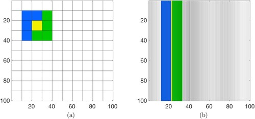5) ) in a computationally tractable manner. Figure 2shows an example of a radiograph with three calibration objects. The first, marked (a), is a ‘step wedge ', which is a block of dense metal cut into steps of different thicknesses used to characterize system response to the X-ray spectrum and fluence. The second, marked (b) in the figure, consists of concentric cylinders of different materials, which are used to calibrate the density reconstruction model. The third object, marked (c) in the figure, is called an ‘L rolled edge ', which can be used to compute the point spread function (see below).

Figure 2. Multi-calibration target consisting of three calibration objects: (a) the step wedge, (b) the Abel cylinder, and (c) the L-rolled edge.

Within the proposed framework, the deblurring problem is defined by (i) the convolution matrix $\mathbf{A}$, (ii) the precision parameters, δ and λ, and (iii) the input data, $\mathbf{b}$. The input data is simply the radiograph. The convolution matrix $\mathbf{A}$ is defined by the deblur kernel, which can be obtained from an appropriate point spread function (PSF). The PSF can be computed from the L rolled edge in Figure 2 [5, 14, 15], and we employ the non-parametric method outlined in [15]. Essentially, by modelling the transition from black to white across the edge as a linear inverse problem, techniques similar to [37] can be used to estimate the PSF's radial profile pixel-by-pixel. This technique has been employed on Cygnus data [15], and that work has been tailored to capture the main components of the Cygnus imaging system's blur. We set small elements in the kernel to zero (by thresholding), to obtain a sparse structure in $\mathbf{A}$ that has a blurring kernel of size $33\times 33$.

The precision parameter λ describes a pixel-wise noise variance, which is calculated as an average variance across the image in Figure 2. Standard deviations of $1.1\times {10}^{-2}$ and $3.4\times {10}^{-3}$ were computed for white and black portions of the image, respectively, so we choose a conservative estimate and set $\lambda =9\times {10}^3$. Motivated by numerical experiments with small portions of the image, we set $\delta =2.5\times {10}^{-3}\cdot \lambda$, based on estimates computed from the Discrepancy Principle [8, 47] and the Unbiased Predictive Risk Estimator [48–50].

4.1. Large-scale image deblurring

The Gibbs sampler described above with a sub-image size of $512\times 512$ (i.e. $8\times 8=64$ sub-images) is applied to deblur the radiograph of size $4096\times 4096$, shown in Figure 2. All computations are performed on one node of the University of Arizona's High Performance Computing (HPC) cluster, which consists of a 2.3 GHz Dual 14-core processor with 192 GBs of memory. On this machine, generating one sample with our code, which does not make use of parallelism, takes about 12 minutes.

Recall that we need to compute the posterior mean to start sampling (see Section 3.5). It is then natural to initialize the Gibbs sampler with the posterior mean which keeps the burn-in period short. See [41] for additional details about the burn-in.

Integrated auto correlation time (IACT) is used to assess the mixing properties of the Markov chain generated by the Gibbs sampler [51]. The IACT defines an effective sample size of a Markov chain by (27) $N_{\mathrm{eff}}\propto N_e/\mathrm{IACT},$(27) where $N_e$ is the length of the Markov chain. Thus, the number of samples required for solving a deblurring problem at a specified accuracy (number of effective samples) is proportional to the IACT. The IACT is computed using techniques described in [52], based on 1000 samples from the posterior. At each pixel, the computed values are between 1 and 10, with an average value of 1.09. The small average IACT indicates that the chain is well-mixed and that nearly all samples are effective samples.

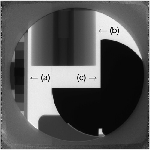
Figure 3 illustrates the results and shows the mean of the 1000 samples along with two zooms, labelled (a) and (b). The mean of the posterior has (i) sharper step edges and a (ii) sharper edge of the concentric cylinders, while transitions within the cylinder remain smooth as expected and desired.

Figure 3. Mean of 1000 samples of the Gibbs sampler. The regions enclosed by red rectangles are shown enlarged on the right.

4.2. Dimension-robustness of the Gibbs sampler

The dimension-robustness of the Gibbs sampler is demonstrated by studying how IACT depends on dimension (putting issues of reaching stationarity to the side). The dimension of the problem is equal to the number of pixels and is thus proportional to the image size. Specifically, IACT defines the number of samples required for solving a deblurring problem at a specified accuracy, or, equivalently, the number of effective samples, via (27(27) $N_{\mathrm{eff}}\propto N_e/\mathrm{IACT},$(27) ). This implies that the number of samples required to characterize the posterior is nearly independent of the size of the image when the IACT is also nearly independent of the size of the image. A dimension-robust algorithm thus must have the property that IACT has little dependence on image size.

To demonstrate dimension-robustness of the Gibbs sampler, we cut smaller images, ranging from $256\times 256$ to $2048\times 2048$, out of the radiograph. The smaller images are centred on a corner of the step wedge to ensure at least one interesting feature exists in each image. We apply the Gibbs sampler, with sub-image size $128\times 128$, to each image and generate 1000 samples. Computing IACT for each image then indicates the scaling of IACT with image size. The results are summarized in Table 1, which lists the mean and maximum (over all pixels) IACT as a function of image size. As the size of the image grows, the IACT has a nearly constant mean IACT and only a modest increase in the maximum IACT. Our numerical experiments thus support dimension-robustness of the Gibbs sampler.

Table 1. Pixel-wise mean and maximum IACTs of the Gibbs sampler as a function of image size.

	Image size
	256	512	1024	2048
Mean IACT:	1.03	1.01	1.02	1.01
Max. IACT:	3.66	3.77	4.23	6.98

The dimension-robustness is also nearly independent of the sub-image size, provided the sub-images are larger than the minimum defined in (13(13) $m_d\ge \frac{m_a-1}{2},n_d\ge \frac{n_a-1}{2}.$(13) ). We demonstrate this property of the Gibbs sampler in numerical experiments in which we vary the image size (from $256\times 256$ to $2048\times 2048$, as above) and the sub-image size (from $256\times 256$ to $1024\times 1024$). The results are summarized in Table 2, which shows the mean and maximum IACT for the various image and sub-image sizes. Both the mean and max IACT are nearly constant for all image and sub-image considered.

Table 2. Average and maximum IACT (in parentheses) as a function of the image size and sub-image size.

	Image size
Sub-image size	$512\times 512$	$1024\times 1024$	$2048\times 2048$
$256\times 256$	1.01 (3.56)	1.02 (4.25)	1.02 (6.56)
$512\times 512$	1	1.01 (3.99)	1.01 (6.26)
$1024\times 1024$	–	1	1.00 (5.11)

4.3. Practical sub-image size

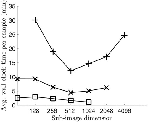
Given the near-independence of image size on the convergence-efficiency of the Gibbs sampler, one may try to find a ‘practical’ sub-image size that leads to the smallest wall clock time required to generate one sample. This was done for the $4096\times 4096$ radiograph in Figure 2 by trying sub-images of size $128\times 128$ (resulting in a $32\times 32$ sub-images) to $2048\times 2048$ (resulting in a $2\times 2$ block of sub-images). Three of the sub-image sizes we tried are illustrated in Figure 4. The average the wall clock time required for a single posterior sample was computed by generating five samples and averaging, and the results are plotted in Figure 5. The lowest wall clock time occurs for sub-images of size $512\times 512$, which is why we used this sub-image size in Section 4.1.

Figure 4. Three different sub-image partitions for an image of size $4096\times 4096$. The sub-images have size $256\times 256$ (left), $512\times 512$ (center) and $1024\times 1024$ (right).

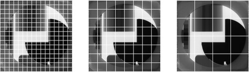
Figure 5 also shows average wall clock times per sample as a function of sub-image size for images of size $1024\times 1024$ and $2048\times 2048$. For the images with $1024\times 1024$ and $2048\times 2048$ pixels, we use the same practical sub-image size ($512\times 512$) as for the $4096\times 4096$ image. The smaller image of size $1024\times 1024$, however, behaves differently in the sense that the practical sub-image size is equal to the full image size. Thus, there is no advantage in using the Gibbs sampler on small images because drawing samples directly, i.e. setting the sub-image size equal to the image size, is feasible and in fact the fastest method. This is in line with our assessment that the proposed Gibbs sampler provides significant computational gains only for large images. Finally, we emphasize that the practical sub-image size also depends on the computing platform used, and a parallelized version of the proposed approach may lead to a different practical sub-image size.

Figure 5. Average wall clock time per sample as a function of sub-image size. Plus signs correspond to an image size of $4096\times 4096$; Xs correspond to an image size of $2048\times 2048$; squares correspond to an image size of $1024\times 1024$.

5. Conclusions

The blocking scheme used to group together variables in a Gibbs sampler has a large effect on its efficiency, in particular in high-dimensional problems. We revisited these ideas in the context of large-scale image deblurring problems, which require drawing samples from Gaussian posterior distributions in ${10}^7$ unknowns.

We constructed a blocking scheme based on sub-images, which respects the 2D nature of imaging problems, and that leads to a sparse and highly structured posterior precision matrix. The Gibbs sampler then naturally exploits this matrix structure during sampling, which makes it dimension-robust, i.e., generating a single sample is feasible and an associated integrated autocorrelation time is nearly independent of the size of the image (the dimension of the problem) in numerical experiments. The dimension-robustness makes the sampler a practical tool for large-scale image deblurring problems.

We demonstrated the applicability of our ideas by implementing and testing the Gibbs sampler on images of size up to $4096\times 4096$ pixels, taken by the Cygnus Dual Beam Radiographic Facility at the Nevada National Security Site. Our implementation is ‘matrix-free’, which is essential, because building and storing precision matrices at the large scale is impractical. Numerical tests demonstrate that the mean pixel-wise integrated autocorrelation time is independent of the size of the image. We also investigated a practical sub-image size that leads to minimal wall clock time per sample on a given computational platform. With a practically chosen sub-image size, the sampler generates $O(100)$ samples in under one day in a $4096\times 4096$ deblurring problem using only modest computational resources. Moreover, the mean reconstructions, generated by the sampler, display sharper features than the blurred image, while still preserving smooth features in the image.

Acknowledgments

The authors would like to thank Johnathan Bardsley for helpful discussions on the algorithm and its applications.

Disclosure statement

No potential conflict of interest was reported by the author(s).

Additional information

Funding

This manuscript has been authored by Mission Support and Test Services, LLC, under Contract No. DE-NA0003624 with the U.S. Department of Energy and supported by the Site-Directed Research and Development Program. The United States Government retains and the publisher, by accepting the article for publication, acknowledges that the United States Government retains a non-exclusive, paid-up, irrevocable, worldwide license to publish or reproduce the published form of this manuscript, or allow others to do so, for United States Government purposes. The U.S. Department of Energy will provide public access to these results of federally sponsored research in accordance with the DOE Public Access Plan (http://energy.gov/downloads/doe-public-access-plan). The views expressed in the article do not necessarily represent the views of the U.S. Department of Energy or the United States Government. DOE/NV/03624–0662. This manuscript was supported by (Pacific Northwest National Labs PNNL-SA-150477).

Notes

1 For the sake of simplicity in indexing, we assume $n_b$ is odd. This is not required, and the formulation holds when $n_b$ is even.

 

Appendix. Summary of notation

We provide a list of frequently used matrices and vectors and their dimensions in Table A1.

Table A1. List of frequently used matrices and vectors.

Explanation	Symbol	Dimension
Image	$\mathbf{B}$	$m_b\times n_b$
Vectorized image	$\mathbf{b}$	$m_b{n}_b\times 1$
Image reconstruction	$\mathbf{X}$	$m_x\times n_x$
Vectorized image reconstruction	$\mathbf{x}$	$m_x{n}_x\times 1$
Sub-image	${\mathbf{X}}_i$	$m_d\times m_d$
Vectorized sub-image	${\mathbf{x}}_i$	$m_d{n}_d\times 1$
Blurring kernel	$\mathbf{a}$	$m_a\times n_a$
Convolution matrix	$\mathbf{A}$	$N\times N$
Cropping matrix	$\mathbf{D}$	$M\times N$
Prior precision matrix	$\mathbf{L}$	$N\times N$
Posterior precision matrix	$\mathbf{H}=\lambda {\mathbf{A}}^{\mathrm{\top }}\mathbf{A}+\delta \mathbf{L}$	$N\times N$
Number of pixels in the image $\mathbf{B}$	$M=m_b\cdot n_b$	–
Number of pixels in the reconstruction $\mathbf{X}$	$N=m_x\cdot n_x$	–
Number of sub-images (vertical & horizontal)	$m_B$, $n_B$	–
Total number of sub-images	$n_p=m_B\cdot n_B$	–

A.1. Matrix-free implementation

We present additional details of the matrix-free implementation of the Gibbs sampler (Section 3.5) and refer to [41] for additional discussion in particular about a careful treatment of the boundaries.

We first discuss the basic functions $f_{{\mathbf{A}}_{:,j}}(\cdot )$, $f_{({\mathbf{A}}_{:,i}{)}^{\mathrm{\top }}}(\cdot )$, $f_{{\mathbf{L}}_{ij}}(\cdot )$ and $f_{{\mathbf{L}}_{ii}^{\mathrm{\top }/2}}(\cdot )$ in (23(23) $\begin{array}{rl}{f}_{{\mathbf{A}}_{:,j}}(\mathbf{y})& ={\mathbf{A}}_{:,j}\mathbf{y},\end{array}$(23) )–(25(25) $\begin{array}{rl}{f}_{{\mathbf{L}}_{ij}}(\mathbf{y})& ={\mathbf{L}}_{ij}\mathbf{y}.\end{array}$(25) ). The function (A1) $f_{{\mathbf{A}}_{:,j}}(\mathbf{y})={\mathbf{A}}_{:,j}\mathbf{y},$(A1) implements the action of the matrix ${\mathbf{A}}_{:,j}$. This action is equivalent to the action of the convolution matrix $\mathbf{A}$, acting on an image with in which only the jth block is nonzero and equal to ${\mathbf{x}}_j$: (A2) ${\mathbf{A}}_{:,j}{\mathbf{x}}_j=\mathbf{A}\left[\begin{array}{c}\mathbf{0}\\ ⋮\\ \mathbf{0}\\ {\mathbf{x}}_j\\ \mathbf{0}\\ ⋮\\ \mathbf{0}\end{array}\right].$(A2) Thus, we can write (A3) $f_{{\mathbf{A}}_{:,j}}({\mathbf{x}}_j)=f_{\mathbf{A}}\left({\left[\begin{array}{ccc}\mathbf{0}& \mathbf{0}& \mathbf{0}\\ \mathbf{0}& {\mathbf{X}}_j& \mathbf{0}\\ \mathbf{0}& \mathbf{0}& \mathbf{0}\end{array}\right]}_{m_x\times n_x}\right),$(A3) where $f_{\mathbf{A}}$ means convolution with the matrix $\mathbf{A}$, and where the $\mathbf{0}$ blocks are appropriately sized so that the ${\mathbf{X}}_j$ block is in the jth position. It is possible to compute just the non-zero portion of $f_{\mathbf{A}}$ and keep track of its location within the image. Implementing $f_{\mathbf{A}}$ in this way means that the zero-padding can be reduced to the size of the kernel, rather than the size of the image. In summary, we implement $f_{{\mathbf{A}}_{:,j}}(\cdot )$ by convolving a small image with a given kernel, which can be implemented efficiently via FFT.

The function (A4) $f_{({\mathbf{A}}_{:,i}{)}^{\mathrm{\top }}}(\mathbf{y})=({\mathbf{A}}_{:,i}{)}^{\mathrm{\top }}\mathbf{y},$(A4) can be implemented similarly. Recall that $\mathbf{A}$ can be written as the product $\mathbf{D}\hat{\mathbf{A}}$. Here $\hat{\mathbf{A}}\in {\mathbb{R}}^{N\times N}$ is the convolution matrix with data-driven boundary conditions, and $\mathbf{D}\in {\mathbb{R}}^{M\times N}$ is the cropping matrix. The transpose, ${\mathbf{A}}^{\mathrm{\top }}={\hat{\mathbf{A}}}^{\mathrm{\top }}{\mathbf{D}}^{\mathrm{\top }}$, first extends the image from size M to size N, and then applies the convolution ${\hat{\mathbf{A}}}^{\mathrm{\top }}$, which is the same as the convolution with the blurring kernel $\mathbf{a}$ flipped in the vertical and horizontal directions.

The function (A5) $f_{{\mathbf{L}}_{ij}}(\mathbf{y})={\mathbf{L}}_{ij}\mathbf{y},$(A5) implements the action of sub-matrices of the negative 2D Laplacian, which is equivalent to convolution with the kernel $\left[\begin{array}{ccc}0& -1& 0\\ -1& 4& -1\\ 0& -1& 0\end{array}\right].$We can thus use the same ideas as above to implement $f_{{\mathbf{L}}_{ij}}(\cdot )$.

Sampling from ${\mathbf{v}}_2\sim \mathcal{N}(\mathbf{0},\delta {\mathbf{L}}_{ii})$ relies on writing the discrete Laplacian as (A6) $\mathbf{L}={\mathbf{D}}_h^{\mathrm{\top }}{\mathbf{D}}_h+{\mathbf{D}}_v^{\mathrm{\top }}{\mathbf{D}}_v,$(A6) where ${\mathbf{D}}_v={\mathbf{D}}_p\otimes {\mathbf{I}}_{m_x}$ and ${\mathbf{D}}_h={\mathbf{I}}_{n_x}\otimes {\mathbf{D}}_p$, and where ⊗ represents the Kronecker product [37]. Here, ${\mathbf{D}}_p$ is the forward difference operator with periodic boundary conditions: (A7) ${\mathbf{D}}_p=\left[\begin{array}{ccccc}-1& 1& 0& \cdots & 0\\ 0& -1& 1& \ddots & ⋮\\ ⋮& \ddots & \ddots & \ddots & 0\\ 0& \ddots & \ddots & -1& 1\\ 1& 0& \cdots & 0& -1\end{array}\right],$(A7) but similar expressions can be derived for zero boundary conditions [41]. Since $\begin{array}{r}{\mathbf{L}}_{ii}=({\mathbf{D}}_h^{\mathrm{\top }}{\mathbf{D}}_h+{\mathbf{D}}_v^{\mathrm{\top }}{\mathbf{D}}_v{)}_{ii}=({\mathbf{D}}_h(:,i){)}^{\mathrm{\top }}{\mathbf{D}}_h(:,i)+({\mathbf{D}}_v(:,i){)}^{\mathrm{\top }}{\mathbf{D}}_v(:,i),\end{array}$sampling ${\mathbf{v}}_2\sim \mathcal{N}(\mathbf{0},\delta {\mathbf{L}}_{ii})$ can be done by writing functions for $({\mathbf{D}}_h(:,i){)}^{\mathrm{\top }}$ and $({\mathbf{D}}_v(:,i){)}^{\mathrm{\top }}$, and constructing ${\mathbf{v}}_2$ as a sum of two independent Gaussians, ${\mathbf{v}}_2={\mathbf{v}}_{2,h}+{\mathbf{v}}_{2,v}$, where ${\mathbf{v}}_{2,h}\sim \mathcal{N}(\mathbf{0},({\mathbf{D}}_h(:,i){)}^{\mathrm{\top }}{\mathbf{D}}_h(:,i))$ and ${\mathbf{v}}_{2,v}\sim \mathcal{N}(\mathbf{0},({\mathbf{D}}_v(:,i){)}^{\mathrm{\top }}{\mathbf{D}}_v(:,i))$. As before, we can sample ${\mathbf{v}}_{2,h}=({\mathbf{D}}_h(:,i){)}^{\mathrm{\top }}\mathbf{z}$, where $\mathbf{z}\sim \mathcal{N}(\mathbf{0},\mathbf{I})$, and ${\mathbf{v}}_{2,v}=({\mathbf{D}}_v(:,i){)}^{\mathrm{\top }}\mathbf{w}$, where $\mathbf{w}\sim \mathcal{N}(\mathbf{0},\mathbf{I})$, $\mathbf{z}$, $\mathbf{w}$ independent. Writing functions for matrix multiplication with $({\mathbf{D}}_h(:,i){)}^{\mathrm{\top }}$ and $({\mathbf{D}}_v(:,i){)}^{\mathrm{\top }}$ is straightforward because the operations (forward differencing and Kronecker products) are elementary (see [41] for details).

We finally comment on the efficient implementation of the pre- and post-sums in (20(20) $f_{\mathrm{pre}}(\mathbf{y},i)=\sum _{j\in {\mathcal{S}}_{\mathrm{pre}}}{\mathbf{H}}_{ij}{\mathbf{y}}_j\mathrm{and}{f}_{\mathrm{post}}(\mathbf{y},i)=\sum _{j\in {\mathcal{S}}_{\mathrm{post}}}{\mathbf{H}}_{ij}{\mathbf{y}}_j.$(20) ), which implement the contributions of the action $\mathbf{H}$ of portions of the neighbouring sub-images to the ith sub-image (see [41] for full details, especially with respect to the treatment of the boundaries). As above, an efficient implementation of these sums exploits the fact that the sum $\sum _{j\in \mathcal{S}}{\mathbf{H}}_{ij}{\mathbf{y}}_j$ can be computed by carefully zero-padding the input, and implementing a functional form of ${\mathbf{H}}_{i,:}=\lambda ({\mathbf{A}}_{:,i}{)}^{\mathrm{\top }}\mathbf{A}+\delta {\mathbf{L}}_{i,:}$ (see [41] for details).

References

- Halls BR, Roy S, Gord JR, et al. Quantitative imaging of single-shot liquid distributions in sprays using broadband flash X-ray radiography. Int J Multiphase Flow. 2016;87:241–249.
- Hanson KM, Cunningham GS. The Bayes inference engine. In: Maximum entropy and Bayesian methods. Dordrecht, The Netherlands: Kluwer Academic; 1996. p. 125–134.
- Howard M, Fowler M, Luttman A, et al. Bayesian Abel inversion in quantitative X-ray radiography. SIAM J Sci Comput. 2016;38:B396–B413.
- Maire E, Withers PJ. Quantitative X-ray tomography. Int Mater Rev. 2014;59:1–43.
- Fowler M, Howard M, Luttman A, et al. A stochastic approach to quantifying the blur with uncertainty estimation for high-energy X-ray imaging systems. Inverse Probl Sci Eng. 2016;24:353–371.
- Nagesh SVS, Rana R, Russ M, Ionita CN, Bednarek DR, Rudin S. Focal spot deblurring for high resolution direct conversion x-ray detectors. Proc SPIE Int Soc Opt Eng. 2016;9783:97833R.
- von Wittenau AES, Logan CM, Aufderheide MB, et al. Blurring artifacts in megavoltage radiography with a flat-panel imaging system: comparison of Monte Carlo simulations with measurements. Med Phys. 2002;29:2559–2570.
- Hansen PC, Nagy JG, O'Leary DP. Deblurring images: matrices, spectra, and filtering. Philadelphia, PA: SIAM; 2006.
- Bardsley JM. Computational uncertainty quantification for inverse problems. Philadelphia (PA): SIAM; 2018.
- Bardsley JM, Luttman A. Dealing with boundary artifacts in MCMC-based deconvolution. Linear Algebra Appl. 2015;473:339–358.
- Bardsley JM, Luttman A. A Metropolis-Hastings method for linear inverse problems with Poisson likelihood and Gaussian prior. Int J Uncertain Quantif. 2016;6:35–55.
- Fox C, Norton RA. Fast sampling in a linear-Gaussian inverse problem. SIAM/ASA J Uncertain Quantif. 2016;4:1191–1218.
- Fox C, Parker A. Accelerated Gibbs sampling of normal distributions using matrix splittings and polynomials. Bernoulli. 2017;23:3711–3743.
- Howard M, Fowler M, Luttman A. Sampling-based uncertainty quantification in deconvolution of X-ray radiographs. J Comput Appl Math. 2014;270:43–51.
- Joyce KT, Bardsley JM, Luttman A. Point spread function estimation in X-ray imaging with partially collapsed Gibbs sampling. SIAM J Sci Comput. 2018;40:B766–B787.
- Wang Z, Bardsley J, Solonen A, et al. Bayesian inverse problems with ℓ1 priors: a randomize-then-optimize approach. SIAM J Sci Comput. 2017;39:S140–S166.
- Parker A, Pitts B, Lorenz L, et al. Polynomial accelerated solutions to a large gaussian model for imaging biofilms: in theory and finite precision. J Am Stat Assoc. 2018;113:1431–1442.
- Chen J, Anitescu M, Saad Y. Computing f(a)b via least squares polynomial approximations. SIAM J Sci Comput. 2011;33:195–222.
- Chow E, Saad Y. Preconditioned krylov subspace methods for sampling multivariate gaussian distributions. SIAM J Sci Comput. 2014;36:A588–A608.
- Parker A, Fox C. Sampling gaussian distributions in krylov spaces with conjugate gradients. SIAM J Sci Comput. 2012;34:B312–B334.
- Gilks W, Richardson S, Spiegelhalter D. Markov chain Monte Carlo in practice. Boca Raton, FL: Springer; 1996.
- Rubinstein RY, Kroese DP. Simulation and the Monte Carlo method. 3rd ed. Hoboken, NJ: Wiley; 2017.
- Morzfeld M, Tong X, Marzouk YM. Localization for MCMC: sampling high-dimensional posterior distributions with local structure. J Comput Phys. 2018;380:1–28.
- Roberts GO, Sahu S. Updating schemes, correlation structure, blocking and parameterization for the Gibbs sampler. J R Stat Soc Ser B. 1997;59:291–317.
- Chen V, Dunlop MM, Papaspiliopoulos O, et al. Dimension-robust MCMC in Bayesian inverse problems. Submitted; 2018.
- Beskos A, Roberts G, Stuart A. Optimal scalings for local Metropolis-Hastings chains on nonproduct targets in high dimensions. Ann Appl Probab. 2009;19:863–898.
- Roberts G, Gelman A, Gilks W. Weak convergence and optimal scaling of random walk Metropolis algorithms. Ann Appl Probab. 1997;7:110–120.
- Roberts G, Rosenthal J. Optimal scaling of discrete approximations to Langevin diffusions. J R Stat Soc, Ser B (Stat Methodol). 1998;60:255–268.
- Buccini A, Donatelli M, Reichel L. Iterated Tikhonov regularization with a general penalty term. Numer Linear Algebra Appl. 2017;24:1–19.
- Chen H, Wang C, Song Y, et al. Split Bregmanized anisotropic total variation model for image deblurring. J Vis Commun Image Represent. 2015;31:282–293.
- Jiao Y, Jin Q, Lu X, et al. Alternating direction method of multipliers for linear inverse problems. SIAM J Numer Anal. 2016;54:2114–2137.
- Ma L, Xu L, Zeng T. Low rank prior and total variation regularization for image deblurring. J Sci Comput. 2017;70:1336–1357.
- Tao S, Dong W, Xu Z, et al. Fast total variation deconvolution for blurred image contaminated by Poisson noise. J Vis Commun Image Represent. 2016;38:582–594.
- Xu J, Chang HB, Qin J. Domain decomposition method for image deblurring. J Comput Appl Math. 2014;271:401–414.
- Bertero M, Boccacci P. A simple method for the reduction of boundary effects in the Richardson-Lucy approach to image deconvolution. Astron Astrophys. 2005;437:369–374.
- Vio R, Bardsley JM, Donatelli M, et al. Dealing with edge effects in least-squares image deconvolution problems. Astron Astrophys. 2005;442:397–403.
- Bardsley JM. Gaussian Markov random field priors for inverse problems. Inverse Probl Imaging. 2013;7:397–416.
- Rue H, Held L. Gaussian Markov random fields: theory and applications. New York, NY: Chapman & Hall/CRC; 2005.
- Gelman A, Carlin JB, Stern HS, et al. Bayesian data analysis. 3rd ed. Boca Raton, FL: Chapman and Hall CRC Press; 2013.
- Geman S, Geman D. Stochastic relaxation, Gibbs distributions, and the Bayesian restoration of images. IEEE Trans Pattern Anal Mach Intell. 1984;PAMI-6:721–741.
- Adams J. Scalable block-Gibbs sampling for image deblurring in X-ray radiography [PhD dissertation]. Tucson (Arizona): University of Arizona; 2019.
- Asaki TJ, Chartrand R, Vixie KR, et al. Abel inversion using total-variation regularization. Inverse Probl. 2005;21:1895–1903.
- Asaki TJ, Campbell PR, Chartrand R, et al. Abel inversion using total variation regularization: applications. Inverse Probl Sci Eng. 2006;14:873–885.
- Davis G, Jain N, Elliott J. A modelling approach to beam hardening correction. Proc SPIE Int Soc Opt Eng. 2008;7078:70781E.
- Kwan TJT, Berninger M, Snell C, et al. Simulation of the cygnus rod-pinch diode using the radiographic chain model. IEEE Trans Plasma Sci. 2009;37:530–537.
- Seeman HE, Roth B. New stepped wedges for radiography. Acta radiol. 1960;53:215–226.
- Engl H, Hanke M, Neubauer A. Regularization for inverse problems. Dordrecht, The Netherlands: Kluwer Academic; 1996.
- Golub GH, Heath M, Wahba G. Generalized cross-validation as a method for choosing a good ridge parameter. Technometrics. 1979;21:215–223.
- Renaut RA, Helmstetter AW, Vatankhah S. Unbiased predictive risk estimation of the tikhonov regularization parameter: convergence with increasing rank approximations of the singular value decomposition. BIT Numer Math. 2019;59:1031–1061.
- Vogel CR. Computational methods for inverse problems. Philadelphia (PA): SIAM; 2002.
- Sokal A. Monte Carlo methods in statistical mechanics: foundations and new algorithms. In: DeWitt-Morette C, Cartier P, Folacci A, editors. Functional Integration. NATO ASI Series (Series B: Physics). Vol. 361. Boston (MA): Springer; 1998.
- Wolff U. Monte Carlo errors with less errors. Comput Phys Commun. 2004;156:145–153.