State estimation problem for the detection of valve closure in gas pipelines

Abstract

The undesired and unexpected closure of valves in pipelines is the most frequent failure that causes interruptions in the transport of natural gas. This work aims at the detection of valve closures by solving a state estimation problem with the Particle Filter method. The gas flow problem in the duct is solved with a Weighted Average Flux – Total Variation Diminishing scheme, while state variables are estimated with simulated measurements of pressure, velocity and temperature at different points along the pipeline. Two versions of the particle filter method are implemented in this work for the solution of the state estimation problem, namely, the Sampling Importance Resampling (SIR) and the Auxiliary Sampling Importance Resampling (ASIR) algorithms. Accurate estimations were obtained with both algorithms for configurations involving pipelines with one or three valves. On the other hand, the SIR algorithm required a larger number of particles than the ASIR algorithm for the same solution accuracy.

KEYWORDS:

• Particle filter
• shutdown valves
• Bayesian framework of statistics
• WAF-TVD scheme
• state estimation problem

Nomenclature

A	=	pipeline cross section area
Cf	=	friction factor
Cp	=	specific heat at constant pressure
Cv	=	specific heat at constant volume
D	=	pipeline diameter
e	=	specific internal energy
$e_{\text{RMS},y}$	=	RMS error for a specific state variable $y(t)$, see equation (12)
f	=	vector of functions that defines the state evolution model
F(t)	=	valve open fraction, $0\le F(t)\le 1$
F(U)	=	flux vector
g	=	vector of functions that define the observation model
I	=	number of measurements at each time instant
n	=	noise vector for the observation model
N	=	number of particles
p	=	pressure
Q	=	local heat flux imposed at the surface of the pipeline
q	=	flow rate
Q	=	covariance matrix of the state evolution model
R	=	covariance matrix of the observation model
Rg	=	gas constant
S(U)	=	source term vector
T	=	temperature
u	=	longitudinal velocity
U	=	vector of conserved variables
v	=	noise vector for the evolution model
w	=	particle weights
x,t	=	spatial and time variables, respectively
y	=	vector of state variables, see equation (6)
${\mathbf{\text{y}}}_{}^{\ast }$	=	reduced vector of state variables, see equation (7)
z	=	measured data predicted with the observation model
${\mathbf{\text{z}}}_{}^{meas}$	=	measurements

Greeks

$\gamma$	=	ratio of specific heats at constant pressure and constant volume ($C_p/C_v$)
$\text{π}$	=	$4{\tan }^{-1}(1)$
$\pi$	=	probability distribution function
$\text{θ}$	=	vector of non-dynamic parameters
ρ	=	density
σ	=	standard deviation

Subscripts

e	=	specific internal energy
k	=	time instant tk
p	=	pressure
ρ	=	density
T	=	temperature
u	=	velocity
v	=	valve number

Superscripts

meas	=	measurements
i	=	particles

Introduction

Worldwide, natural gas is mainly transported through pipelines from production sites to treatment units, as well as from treatment units to industrial and domestic consumers.For safety reasons, automatic shutdown valves (denoted as SDVs) are installed along pipelines. These valves avoid, for example, gas scape through leakages caused by accident or illegal tampering, by automatically closing sections of the pipeline. The number and positions of SDVs along the pipeline depend on several factors, including proximity to highly populated areas. Usually, SDVs are located between 8 and 30 km apart from each other. The automatic closure of SDVs is set in accordance with the pipeline operational limits. Transients in the gas flow may cause pressure variations that result on the sudden and undesired closure of SDVs, due to unexpected modifications in the flow rates demanded by big consumers. A numerical solution for the pressure wave propagation in gas pipelines after the sudden closure of a shutdown valve was presented in [1].

Automatic shutdown valves are not remotely operated or monitored, because of the high costs of dedicated sensors and actuators. Therefore, an undesired and unexpected closure of these valves is usually detected empirically by operators at pipeline operational centres, based on their own practical experiences. From the pressure and flow rate readings at measurement stations along the pipeline, operators can identify a region containing the closed SDV. In general, pressure increases and flow rate decreases upstream of the closed valve, while pressure decreases downstream. After the identification of the pipeline region where the unexpected closed SDV is possibly located, technicians are assigned for in-situ verification of all valves in this region until the closed one is found and reopen. This process may take few hours, depending on the number and distance of SDVs, as well as their location with respect to main roads, thus incurring in large financial losses and operational problems for large industrial consumers, such as power plants. Therefore, the development of numerical tools for the automatic and fast identification of the closure of SDVs, with minimum interference by the pipeline operators, is of great importance.

In this paper, we apply state estimation techniques to identify the undesired and unexpected closure of automatic shutdown valves. In state estimation problems, physical phenomena are taken into account by a state evolution model and an observation model [2–14]. The information provided by these two stochastic models, as well as by the measured data, is used to sequentially estimate the desired dynamic variables in such a manner that the estimation error is statistically minimized. The Kalman filter provides the optimal solution for state estimation problems with linear models and additive Gaussian noises, by recursively applying analytic equations [2–5]. The Kalman filter was applied as an observer for the control of gas pipelines in [15] and to detect valve stiction in [16,17]. Unfortunately, many practical applications, such as the one under analysis in this work, involve nonlinear and/or non-Gaussian models, for which the original Kalman filter cannot be applied. The so-called Particle Filter methods provide a powerful and robust technique for the solution of nonlinear and/or non-Gaussian estimation problems, with results more accurate than those obtained with the available extensions of the Kalman filter [2–14] for innumerous practical applications [18–25]. Several algorithms for the implementation of the particle filter method can be found in the literature [2–5]. In this work, two of these algorithms are compared, as applied to the estimation of SDV closures with computer simulated measurements, namely: the Sampling Importance Resampling (SIR) algorithm and the Auxiliary Sampling Importance Resampling (ASIR) algorithm [2–5].

The model for the compressible fluid flow of the gas inside the pipeline is presented in the next section, which is followed by the definition of the state estimation problem and its solution based on the particle filter method. The SIR and ASIR algorithms of the particle filter are then presented and the solution of the state estimation problem is obtained with computer simulated measurements.

Mathematical formulation

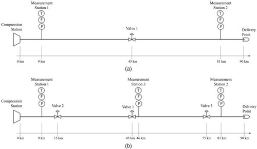
Two configurations were examined in this work for a straight and horizontal pipeline without bifurcations, with length of 90 km between the compression station and the point where the gas was delivered for consumption. The diameter of the pipeline was D = 18 inch. For configuration 1, one single automatic shutdown valve was located at the position x = 45 km. For configuration 2, three automatic shutdown valves were located at positions x = 15 km, x = 45 km and x = 75 km. Sensors for temperature, pressure and flow rate were located at x = 9 km and x = 81 km. In addition, sensors were also located at x = 46 km for configuration 2. The idealized configuration 1 was used as a test case for verification purposes and for the comparison of the two particle filter algorithms examined in this work. Configuration 2 more closely reflects cases found in practice, with three SDV’s located 30 km apart. These two configurations are illustrated by Figure 1a and 1b, respectively.

Figure 1. Sketch of the straight pipeline for: (a) Configuration 1 with one SDV and (b) Configuration 2 with three SDVs.

The physical problem is modelled by the one-dimensional compressible flow of an ideal gas with constant specific heat, in an horizontal and straight pipeline. The mass, momentum and energy conservation equations for this problem can be written in vector form as [26,27]: (1) $\frac{\mathrm{\partial }\mathbf{\text{U}}}{\mathrm{\partial }t}+\frac{\mathrm{\partial }\mathbf{\text{F}}(\mathbf{\text{U}})}{\mathrm{\partial }x}=\mathbf{\text{S}}(\mathbf{\text{U}})$(1) where (2a-c) $\begin{array}{r}\mathbf{\text{U}}\equiv \left[\begin{array}{c}\rho \\ \rho u\\ \rho \left(e+{\displaystyle \frac{u^2}{2}}\right)\end{array}\right]\mathbf{\text{F}}(\mathbf{\text{U}})\equiv \left[\begin{array}{c}\rho u\\ \rho u^2+p\\ \rho u\left(e+{\displaystyle \frac{u^2}{2}}+{\displaystyle \frac{p}{\rho }}\right)\end{array}\right]\mathbf{\text{S}}(\mathbf{\text{U}})\equiv -{\displaystyle \frac{1}{A}}\left[\begin{array}{c}0\\ \rho u^2{\displaystyle \frac{C_f\text{π}D}{2}}\\ -Q\text{π}D\end{array}\right]\end{array}$(2a-c) In equations (1) and (2), U, F(U) and S(U) are the vectors of conserved variables, fluxes and source terms, respectively, while ρ is the density, u is the longitudinal velocity, e is the specific internal energy, p is the pressure, Q is the local heat flux imposed at the surface of the pipeline, A is the cross section area and C_f is the friction factor. The equations of state for an ideal gas are given by: (3a,b) $p=(\gamma -1)\rho eT=\frac{p}{\rho R_g}$(3a,b) where $\gamma =C_p/C_v$, C_v is the specific heat at constant volume, C_p is the specific heat at constant pressure, T is the temperature and R_g is the gas constant.

Several works can be found in the literature for the numerical solution of the gas flow in a single pipeline and in pipeline networks. In particular, the reader is referred to references [1,28–34]. Here, we apply the Total Variation Diminishing (TVD) Weighted Average Flux (WAF) scheme presented by Toro [35] for the solution of equations (1) to (3), by using the Van Leer limiting function and the HLLC method for the approximate Riemann solver. Details of this finite volume scheme are omitted here for the sake of brevity, but they can be readily found in standard textbooks [35,36].

The analytical boundary conditions for a well-posed one-dimensional flow problem need to be specified as follows [37]: (i) Subsonic Inlet: Density, ρ, needs to be prescribed. Thus, one can prescribe the sets [ρ, u] or [ρ, p], but not [p, u]. Note that one can also specify [T, p], because temperature and pressure are more easily measured, which in turn signifies that [ρ, p] are prescribed, since ρ is related to T and p by the equation of state (3b); (ii) Subsonic Outlet: One of the three variables, ρ, u or p, needs to be prescribed; (iii) Supersonic Inlet: The three variables ρ, u and p need to be prescribed; (iv) Supersonic Outlet: No variable needs to be prescribed. For the numerical integration of equations (1) to (3) with the WAF-TVD scheme, scalars need to be specified in fictitious volumes at the pipeline inlet and outlet. Extrapolations from the interior volumes to the fictitious volumes were then performed in accordance with the flow conditions, as described by [35–38] and summarized by Table 1. For all cases, ρ and e were calculated with the equations of state (3a,b). The initial conditions for the integration of equations (1) to (3) will be described below in the section of Results and Discussions.

Table 1. Numerical boundary conditions.

	Inlet		Outlet
	Subsonic	Supersonic	Subsonic	Supersonic
Prescribed	p and T	p, T and u	u	No variables
Extrapolated	u	No variables	p and T	p, T and u

The automatic shutdown valves were modelled by following [39,40] in accordance with the ISA standard [41]. The flow rate at each valve was computed by: (4a) $q=N_7{F}_p{c}_v{P}_{up}Y\sqrt{\frac{\chi }{S_G{T}_{up}Z}}$(4a) where (4b,c) $Y=1-\frac{\chi }{3{\varphi }_k{\chi }_t}\chi =\frac{\mathrm{\Delta }P}{P_{up}}$(4b,c) In equations (4a-c), N₇ = 4.17 K^0.5Pa^−0.5 for SI Units, F_p is a factor that accounts for the geometrical variation between the pipe and the valve, $c_v$ is the valve flow coefficient, Y is an expansion coefficient given by equation (4b), $\chi$ is the valve pressure drop (ΔP) relative to the valve upstream pressure ($P_{up}$) given by equation (4c), S_G is the specific gravity of the gas with respect to air at standard conditions, $T_{up}$ is the valve upstream gas temperature, Z is the gas compressibility factor, ${\varphi }_k$ is the ratio between $\gamma (C_p/C_v)$ for the gas and for air, while ${\chi }_t$ is the ratio $\chi$ (equation 4c) for the chocked flow through the valve [39].

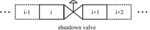
For the numerical solution of the flow problem, each shutdown valve was modelled between two control volumes with interfaces at the valve position, as shown in Figure 2 [30]. The valve flow rate was supposed proportional to the valve opening. Therefore, the flow rate given by equation (4a) was multiplied by a function of time F(t) that represented the valve opening, where $0\le F(t)\le 1$. By following the explicit scheme of the WAF-TVD method, the flow rate through each valve was calculated with equations (4a-c) by using the variables at the previous time step.

Figure 2. Sketch of valve between two consecutive discrete control volumes.

The numerical code developed in this work for the WAF-TVD solution of the gas flow problem was verified by using the analytic solutions for the Fanno and Rayleigh lines, as well as for the shock tube problem [26,27]. Relative differences between the numerical and analytic solutions were less than 0.6% with 100 volumes in the discretization, where the integration time step was automatically selected by satisfying the stability criterion of the WAF-TVD scheme [35].

Real gas effects can be significant at pressures commonly observed in natural gas pipelines. On the other hand, the ideal gas model is followed here as in [29], since the objective of this work is to detect the closure of shutdown valves by solving a state estimation problem. However, we note that a compressibility factor that depends on the natural gas composition could be included in the formulation to model a real gas [32,33].

State estimation problems and particle filters

State estimation problems involve two stochastic mathematical models: the evolution model, which represents the discrete time variation of the state variables, and the observation model, which provides a relationship between the measurements and the state variables [2–14]. The state variables are given by the vector ${\mathbf{\text{y}}}_k$, which describe the system at a given time instant $t_k$. The state evolution model and the observation model are defined by the functions ${\mathbf{\text{f}}}_k$ and ${\mathbf{\text{g}}}_k$, respectively, and can be written in the following general nonlinear forms [2–14]: (5a) $\begin{array}{rl}{\mathbf{\text{y}}}_k& ={\mathbf{\text{f}}}_k({\mathbf{\text{y}}}_{k-1},\text{θ},{\mathbf{\text{v}}}_k),k=1,\dots ,M\end{array}$(5a) (5b) $\begin{array}{rl}{\mathbf{\text{z}}}_k& ={\mathbf{\text{g}}}_k({\mathbf{\text{y}}}_k,\text{θ},{\mathbf{\text{n}}}_k),k=1,\dots ,M\end{array}$(5b) where ${\mathbf{\text{z}}}_k$ is the prediction of the measurements, $\text{θ}$ is a vector containing all the non-dynamic parameters of the model, while ${\mathbf{\text{v}}}_k$ and ${\mathbf{\text{n}}}_k$ represent the noises in the state evolution model and in the observation model, respectively. The objective of the state estimation problem is to obtain information about the state vector ${\mathbf{\text{y}}}_k$ based on the measurements, as well as on the evolution and observation models defined by equations (5a,b), respectively, with known probability density $\pi ({\mathbf{\text{y}}}_0,\text{θ}|{\mathbf{\text{z}}}_0)=\pi ({\mathbf{\text{y}}}_0,\text{θ})$ at the initial time t = 0 [2–14].

In this work, the particle filter method was applied for the solution of the present nonlinear state estimation problem. This method is a sequential Monte Carlo technique, where the posterior probability density function of the state variables is represented by a set of random samples (particles) with associated weights. We denote the particles by ${\mathbf{\text{y}}}_k^i$ and their corresponding weights by $w_k^i,i=1,\dots ,N$.

Basic steps of the particle filter method can be summarized as follows. From the distribution at the initial time, $\pi ({\mathbf{\text{y}}}_0,\text{θ}|{\mathbf{\text{z}}}_0)=\pi ({\mathbf{\text{y}}}_0,\text{θ})$, a prior information for the state variables at the subsequent time, $t_1$, is estimated by using the state evolution model given by equation (5a). The observation model given by equation (5b) and the actual measurements, ${\mathbf{\text{z}}}_k^{meas}$, are then used in the likelihood function (the statistical model for the measurement errors) to compute the weights for the particles. This process is repeated for the estimation of state variables at future times, as the measured data is sequentially assimilated. Although simple, after few time steps such a recursive application of Bayes’ theorem might degenerate the particles. The degeneracy phenomenon is characterized by most of the particles with negligible weights, which implies that a large computational effort is devoted to update particles whose contribution to the approximation of the posterior density function is almost zero. The degeneracy phenomenon can be overcome with a resampling step in the particle filter, which eliminates particles with small weights and generates new particles from those with large weights [2,4,5]. Resampling can be performed if the number of particles with large weights falls below a certain threshold number. Alternatively, resampling can be performed at every time step, such as in the Sampling Importance Resampling (SIR) algorithm [4,5]. Although the resampling step reduces the effects of degeneracy, it may lead to a loss of diversity and the resultant sample may contain many repeated particles [2,4,5]. The Auxiliary Sampling Importance Resampling (ASIR) algorithm was developed with the objective to reduce sample impoverishment, by applying the resampling step at time $t_{k-1}$with the measurements at time $t_k$ [2,4,5]. The resampling step is based on some point estimate ${\mathit{\mu }}_k^i$ that characterizes $\pi ({\mathbf{\text{y}}}_k^i|{\mathbf{\text{y}}}_{k-1}^i,\text{θ})$, which can be the mean or a sample of this distribution. The Sampling Importance Resampling (SIR) algorithm and the Auxiliary Sampling Importance Resampling (ASIR) algorithm are presented by Tables 2 and 3, respectively, for the evolution of the system from time $t_{k-1}$to $t_k$ [4,5].

Table 2. Sampling importance resampling (SIR) algorithm [4,5].

Step 1

For $i=1,\dots ,N$ draw new particles ${\mathbf{y}}_k^i$ from the prior density $\pi ({\mathbf{y}}_k^i|{\mathbf{y}}_{k-1}^i,\text{θ})$and then use the likelihood density to calculate the corresponding weights $w_k^i=\pi ({\mathbf{z}}_k^{meas}|{\mathbf{y}}_k^i,\text{θ})$.

Step 2

Calculate the total weight $T_w=\sum _{i=1}^N{w}_k^i$ and then normalize the particle weights, that is, for $i=1,\dots ,N$ let $w_k^i=T_w^{-1}{w}_k^i$.

Step 3

Resample the particles as follows:

Construct the cumulative sum of weights (CSW) by computing $c_i=c_{i-1}+w_k^i$ for $i=1,\dots ,N$, with $c_0=0$.

Let $i=1$ and draw a starting point $u_1$ from the uniform distribution $U[0,N^{-1}]$

For $j=1,\dots ,N$

Move along the CSW by making $u_j=u_1+N^{-1}(j-1)$

While $u_j>c_i$ make $i=i+1$ and

Assign sample ${\mathbf{y}}_k^j={\mathbf{y}}_k^i$

Assign sample weight $w_k^j=N^{-1}$

Table 3. Auxiliary sampling importance resampling (ASIR) algorithm [4,5].

Step 1

For $i=1,\cdots ,N$, draw new particles ${\mathbf{y}}_k^i$ from the prior density $\pi ({\mathbf{y}}_k^i|{\mathbf{y}}_{k-1}^i,\text{θ})$ and calculate some point characteristic ${\mathit{\mu }}_k^i$ of ${\mathbf{y}}_k^i$, given ${\mathbf{y}}_{k-1}^i$ and $\text{θ})$. Then, use the likelihood density to calculate the corresponding weights $w_k^i=w_{k-1}^i\pi ({\mathbf{z}}_k^{meas}|{\mathit{\mu }}_k^i,\text{θ})$.

Step 2

Calculate the total weight $T_w=\sum _{i=1}^N{w}_k^i$ and then normalize the particle weights, that is, for i = 1, … ,N let $w_k^i=T_w^{-1}{w}_k^i$.

Step 3

Resample the particles as follows:

Construct the cumulative sum of weights (CSW) by computing  $c_i=c_{i-1}+w_k^i$ for i = 1, … ,N, with $c_0=0$.

Let i = 1 and draw a starting point $u_1$ from the uniform distribution $U[0,N^{-1}]$.

For $j=1,\dots ,N$:

Move along the CSW by making $u_j=u_1+N^{-1}(j-1)$

While $u_j>c_i$ make $i=i+1$

Assign sample ${\mathbf{x}}_{k-1}^j={\mathbf{x}}_{k-1}^i$

Assign parent $i^j=i$

Step 4

For $j=1,\cdots ,N$draw particles ${\mathbf{y}}_k^j$ from the prior density $\pi ({\mathbf{y}}_k^j|{\mathbf{y}}_{k-1}^{i^j},\text{θ})$, using the parent $i^j$, and then use the likelihood density to calculate the correspondent weights $w_k^j=\pi ({\mathbf{z}}_k^{\mathit{\text{meas}}}|{\mathbf{y}}_k^j,\text{θ})/\pi ({\mathbf{z}}_k^{\mathit{\text{meas}}}|{\mathit{\mu }}_k^{i^j},\text{θ})$.

Step 5

Calculate the total weight $T_w=\sum _{j=1}^N{w}_k^j$ and then normalize the particle weights, that is, for $j=1,\cdots ,N$ let $w_k^j=T_w^{-1}{w}_k^j$.

The SIR and ASIR algorithms of the particle filter method were applied below for the estimation of unexpected closures of shutdown valves, in the configurations presented in Figure 1a,b. Therefore, the vector of state variables is composed by the dependent variables of the flow model given by equations (1) to (3), as well as by the functions F_v(t) that represent the open fraction of each valve v, where v = 1 for configuration 1, and v = 1, 2 and 3 for configuration 2. In discrete form, we have: (6) $\mathbf{\text{y}}=\left[\begin{array}{c}\mathit{\rho }\\ \mathbf{\text{u}}\\ \mathbf{\text{e}}\\ \mathbf{\text{T}}\\ \mathbf{\text{p}}\\ \mathbf{\text{F}}\end{array}\right]$(6) where the vectors ρ, u, e, T and p contain the density, velocity, internal energy, temperature and pressure, respectively, at all finite volumes used for the discretization of the pipeline. The vector F contains the open fractions of the valves in the pipeline. Hence, F is a scalar for configuration 1 and a vector of size [3 × 1] for configuration 2.

The evolution models for (7) ${\mathbf{\text{y}}}_k^{\ast }=\left[\begin{array}{c}{\mathit{\rho }}_k\\ {\mathbf{\text{u}}}_k\\ {\mathbf{\text{e}}}_k\\ \begin{array}{l}{\mathbf{\text{T}}}_k\\ {\mathbf{\text{p}}}_k\end{array}\end{array}\right]$(7) were given by equations (1) to (3) discretized with the WAF-TVD scheme, which are represented by the vector ${\mathbf{\text{f}}}_k^{\ast }({\mathbf{\text{y}}}_{k-1}^{},\text{θ})$ in equation (8). Uncertainties for these state variables were supposed additive, uncorrelated, Gaussian, with zero means and constant covariance matrix, Q. Therefore, for the computation of the state variables ${\mathbf{\text{y}}}_k^{\ast }$ at a time $t_k^{}$, we can write (8) ${\mathbf{\text{y}}}_k^{\ast }={\mathbf{\text{f}}}_k^{\ast }({\mathbf{\text{y}}}_{k-1},\text{θ})+{\mathbf{\text{v}}}_k^{\ast }$(8) where ${\mathbf{\text{v}}}_k^{\ast }=N(\mathbf{0},\mathbf{\text{Q}})$.

No information was a priori assumed for the functional form of the vector F, which gives the open fractions of the valves in the pipeline. Therefore, the evolution models for these state variables were given by independent Markovian processes with Gaussian distributions, zero means and variances ${\sigma }_{v,k}^2$, that is, (9) $F_{v,k}^{}=F_{v,k-1}^{}+{\sigma }_{v,k}^{}{\phi }_{v,k}$(9) where ${\phi }_{v,k}$ is a random Gaussian number with zero mean and unitary standard deviation.

Measurements of pressure, temperature and flow rate were supposed available at the positions illustrated by Figure 1a,b. Flow rate measurements were considered here as velocity measurements. Therefore, the function ${\mathbf{\text{g}}}_k({\mathbf{\text{y}}}_k,\text{θ},{\mathbf{\text{n}}}_k)$, in the observation model given by equation (5b), selected the pressure, temperature and velocity at the measurement positions from the vector of state variables ${\mathbf{\text{y}}}_k^{\ast }$. The measurements were supposed uncorrelated and containing additive Gaussian noises, with zero means and constant covariance matrix, R. The standard deviations in the measurements of u, T and p are given by ${\sigma }_u^{\mathit{\text{meas}}}$, ${\sigma }_T^{\mathit{\text{meas}}}$ and ${\sigma }_p^{\mathit{\text{meas}}}$, respectively. Therefore, the observation model can be written as (10) ${\mathbf{\text{z}}}_k={\mathbf{\text{g}}}_k({\mathbf{\text{y}}}_k^{\ast },\text{θ})+{\mathbf{\text{n}}}_k$(10) where ${\mathbf{\text{n}}}_k^{}=N(\mathbf{0},\mathbf{\text{R}})$.

With these hypotheses about the measurement errors, the likelihood function, which is used for the computation of the weights in the particle filter method, is thus given by: (11) $\begin{array}{r}\pi ({\mathbf{\text{z}}}_k|{\mathbf{\text{y}}}_k^{},\text{θ})=(2\text{π}{)}^{-I/2}|\mathbf{\text{R}}{|}^{-1/2}exp\left\{-\frac{1}{2}{[{\mathbf{\text{z}}}_k^{meas}-{\mathbf{\text{g}}}_k({\mathbf{\text{y}}}_k^{\ast },\text{θ})]}^T{\mathbf{\text{R}}}^{-1}[{\mathbf{\text{z}}}_k^{meas}-{\mathbf{\text{g}}}_k({\mathbf{\text{y}}}_k^{\ast },\text{θ})]\right\}\end{array}$(11) where I is the number of measurements at each time instant, $t_k^{}$, and $\text{π}=4{\tan }^{-1}(1)$.

The vector of model parameters, $\text{θ}$, was supposed known in this work, but their related uncertainties were accounted for in the vectors ${\mathbf{\text{v}}}_k^{\ast }$and ${\mathbf{\text{n}}}_k^{}$.

Results and discussions

For the results presented below, the time period for the analysis of the gas flow corresponded to one hour of physical time. The pipeline was considered thermally insulated, that is, Q = 0 W/m², and the friction factor was taken as 0.005 [26] for the flow of air. The pressure and the temperature imposed at the inlet boundary were 6.5 × 10⁶ Pa and 298 K, respectively, while the velocity imposed at the outlet boundary was 6 m/s. Initial conditions were taken from the Fanno line, which resulted from the outflow velocity specified as the boundary condition when the outlet pressure was 3.8 × 10⁶ Pa. We assumed in this work that the valve and the pipe were of the same diameter, so that F_p = 1, and, for an ideal gas, Z = 1. Moreover, for air ${\varphi }_k=S_G=1$ and ${\chi }_t=0.75$ [39]. The valve flow coefficient was considered as $c_v=6.7\times {10}^{-6}{\text{m}}^3{\text{s}}^{-1}\text{P}{\text{a}}^{-0.5}$ [39].

For the solution of the state estimation problem, the measurements were supposed available every 72 s, which is in accordance with SCADA systems used in practice. Therefore, during the period of one hour, M = 50 measurements obtained with each sensor were used for the estimation of the state variables and the detection of the valve closure. The sudden closure of either one of the shutdown valves was supposed to occur at time t = 20 minutes. The full closure was assumed instantaneous. Based on sensors used in pipelines nowadays, the standard deviations for the measurements of velocity, temperature and pressure were taken as ${\sigma }_u^{\mathit{\text{meas}}}=0.2\text{m/s}$, ${\sigma }_T^{\mathit{\text{meas}}}=0.5\text{K}$ and ${\sigma }_p^{\mathit{\text{meas}}}=2\times {10}^4\text{Pa}$, respectively. Standard deviations for the evolution models of these state variables were assumed as twice as large, in order to account for uncertainties in the model parameters, $\text{θ}$, that is, ${\sigma }_u^{}=0.4\text{m/s}$, ${\sigma }_T^{}=1\text{K}$ and ${\sigma }_p^{}=4\times {10}^4\text{Pa}$. For the random walk evolution model of the valve open fraction, given by equation (9), the standard deviation ${\sigma }_{v,k}^{}$ was taken as $0.1F_{v,k-1}$. This quantity was selected with numerical experiments and provided stable solutions with fast response times.

The accuracies of the solutions of the state estimation problems were examined with the RMS error, which is defined for a specific state variable $y(t)$as: (12) $e_{\text{RMS},y}=\sqrt{\frac{1}{M}\sum _{k=1}^M{[\overline{y}(t_k)-y_{\text{exact}}(t_k)]}^2}$(12) where, at time $t_k$, $y_{\text{exact}}(t_k)$ is the exact value of the state variable y(t), while $\overline{y}(t_k)$ is the mean estimated by the particle filter method with particles $y_k^i$ and their corresponding weights $w_k^i,i=1,\dots ,N$ (see Tables 2 and 3), that is, (13) $\overline{y}(t_k)=\sum _{i=1}^N{w}_k^i{y}_k^i$(13) The results obtained with the SIR and ASIR algorithms are compared below by using computer simulated measurements. The simulated measurements were obtained from the numerical solution of the forward problem, by considering Gaussian uncorrelated errors with the same standard deviations of the observation model.

Configuration 1

The RMS errors for the valve open fraction (given in percentage), as well as for pressure, temperature and velocity at the measurement positions x = 9 km and x = 81 km, are presented in Table 4, for configuration 1 (see Figure 1a). These errors are presented for the results obtained with the particle filter algorithms SIR and ASIR, by using different numbers of particles. Computational times are also presented in this table and they refer to Matlab® codes run in a computer with a processor Intel® Core™i7(2600) 3.6 GHz and 8 GByte of RAM memory.

Table 4. RMS errors and computational times for configuration 1.

Algorithm			SIR				ASIR
Number of Particles			100	200	500	1000	100	200	500
Computational Time (h)			3	5	17	40	9	15	26
RMS	Valve opening	[%]	33.05	32.59	31.62	30.77	28.04	27.32	28.03
Errors	Pressure at x = 9 km	[kPa]	19.67	24.09	15.05	15.97	13.19	9.97	12.93
	Pressure at x = 81 km	[kPa]	65.50	47.33	46.19	43.41	25.91	24.36	19.64
	Velocity at x = 9 km	[m/s]	0.733	0.792	0.446	0.459	0.262	0.261	0.245
	Velocity at x = 81 km	[m/s]	0.178	0.181	0.128	0.120	0.091	0.076	0.089
Temperature at x = 9 km	[K]	1.341	1.385	1.048	0.703	0.345	0.520	0.524
Temperature at x = 81 km	[K]	1.859	1.317	1.262	0.837	0.521	0.581	0.489

An analysis of Table 4 reveals that the RMS errors obtained with the ASIR algorithm were in general smaller than those obtained with the SIR algorithm. The RMS errors of the SIR algorithm exhibited an asymptotic behaviour for more than 500 particles, but the RMS errors were practically constant in the ASIR algorithm for more than 100 particles. The RMS errors of the ASIR algorithm with only 100 particles were smaller than those of the SIR algorithm with 1000 particles. As expected, the computational times were larger for the ASIR algorithm than for the SIR algorithm, by considering the same number of particles. Such was the case because the forward problem was solved twice at each evolution of the filter with the ASIR algorithm, but solved only once with the SIR algorithm, as shown by Tables 2 and 3. On the other hand, the ASIR algorithm with 100 particles was about four times faster than the SIR algorithm with 1000 particles.

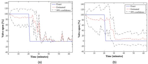
Figures 3a and 3b present the exact and estimated valve open percentages (means given by equation 13), obtained with 1000 particles in the SIR algorithm and with 100 particles in the ASIR algorithm, respectively, as well as the 99% confidence intervals of the estimates. These figures show that the ASIR estimates were smoother and more accurate than those of the SIR algorithm. Differently from the estimates obtained with the SIR algorithm, the ASIR results did not exhibit sample impoverishment, which is characterized by very small confidence intervals. Such was the case because resampling was performed at the previous time by using the measurements at the current time in the sequential estimation with the ASIR algorithm (see Table 3). Figure 3b shows that in about eight minutes of physical time the ASIR algorithm could detect the valve closure with 99% confidence. Hence, the ASIR algorithm responded fast for detecting the valve closure. We note that the accurate estimations presented by Figures 3a,b were obtained without any prior information regarding the valve open fraction, which was modelled by the random walk evolution model given by equation (9).

Figure 3. Valve open percentage estimated for configuration 1 with: (a) 1000 particles in the SIR algorithm and (b) 100 particles in the ASIR algorithm.

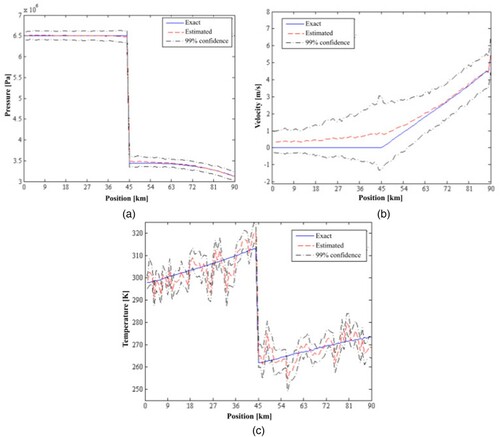
A comparison of simulated measurements and state variables estimated with the ASIR algorithm with 100 particles is presented in Figures 4a-f. The exact variables, which were used to generate the simulated measurements, are also presented in Figures 4a-f. These figures show an excellent agreement between estimated and exact variables, despite the large measurement errors considered in the analysis. Indeed, the ASIR algorithm of the particle filter was capable of providing accurate estimates even for state variables for which measurements were not available. Such fact is apparent from the analysis of Figures 5a-c, which present the exact and the estimated pressure, velocity and temperature along the pipeline, respectively, at the final time.

Figure 4. Simulated measurements, exact and estimated state variables obtained with 100 particles in the ASIR algorithm for configuration 1: (a) Pressure at x = 9 km, (b) Pressure at x = 81 km, (c) Velocity at x = 9 km, (d) Velocity at x = 81 km, (e) Temperature at x = 9 km, (f) Temperature at x = 81 km.

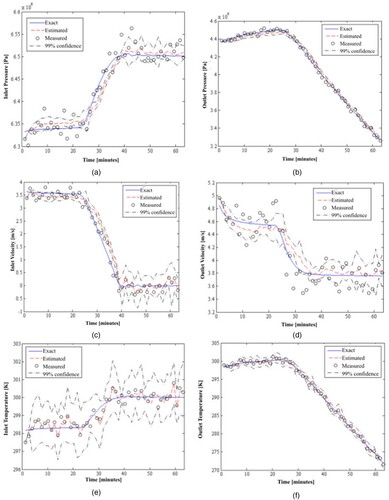
Figure 5. Exact and estimated state variables along the pipeline at the final time, obtained with 100 particles in the ASIR algorithm for configuration 1: (a) Pressure, (b) Velocity, (c) Temperature.

Configuration 2

For this configuration involving three shutdown valves (see Figure 1b), two cases were examined regarding the number of stations where measurements were assumed available for the solution of the state estimation problem, namely: (i) Two measurement stations, at x = 9 km and x = 81 km; and (ii) Three measurement stations, at x = 9 km, x = 46 km and x = 81 km. After the above comparison of the particle filter algorithms for configuration 1, only the results obtained with the ASIR algorithm are now presented for configuration 2. The results presented below were obtained with 200 particles.

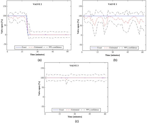
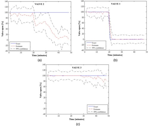
We consider first the case with two measurement positions, where valve 2 was suddenly closed while the others were maintained fully open. Figures 6a-c present the estimated open percentages for the three valves and their related 99% confidence intervals, together with the exact functional forms used to generate the simulated measurements. We notice in Figures 6a-c that excellent estimates were obtained for the open percentages of valves 2 and 3. The estimated open percentage of valve 1 was oscillatory and with uncertainties larger than those for the other valves, as shown by Figure 6b. This behaviour resulted from the fact that valves 2 and 3 were near the measurement stations, but valve 1 was located in the middle of the pipeline and quite far from the measurement stations. However, the exact open percentage of valve 1 was found within the 99% confidence interval of the estimations obtained with the ASIR algorithm of the particle filter.

Figure 6. Exact and estimated valve open percentages obtained for valve 2 closed and the other valves fully open, in configuration 2 with two measurement stations: (a) Valve 2; (b) Valve 1; (c) Valve 3.

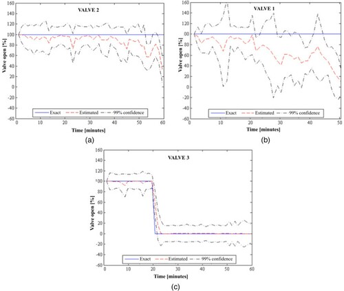
The sudden closure of valve 3 could also be accurately estimated by using the measurements of stations 1 and 2, as demonstrated by Figures 7a-c. On the other hand, these figures show that the open percentages estimated for valves 1 and 2 were oscillatory and tended to zero near the final time. These behaviours for valves 1 and 2 were due to the decreasing flow rate upstream of the closed valve, where the pressure tended to be constant and equal to the value assigned at the inlet boundary condition. Hence, the measurements at station 1 near the pipeline inlet gradually lost sensitivity with respect to which valve was closed and the estimated open percentages of valves 1 and 2 deteriorated. However, Figures 7a-c show that the estimation of the closure of valve 3 could be accurately identified in less than five minutes, while the open percentages of valves 1 and 2 tended to zero in about thirty minutes after the closure of valve 3. Moreover, the estimation of the open percentage of valve 3 was more stable than those for the other upstream valves. Therefore, in a real situation the operator could easily detect that the closures estimated for the upstream valves 1 and 2 resulted from the actual closure of valve 3.

Figure 7. Exact and estimated valve open percentages obtained for valve 3 closed and the other valves fully open, in configuration 2 with two measurement stations: (a) Valve 2; (b) Valve 1; (c) Valve 3.

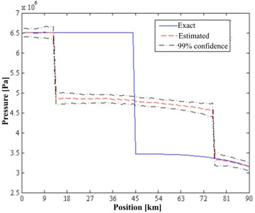
Differently from the cases presented by Figures 6 and 7, which involved the closure of valves near the measurement positions, the closure of valve 1 (with the other valves fully open) could not be accurately estimated by using the measurements from only two stations. Figures 8a-c compare the exact and estimated valve open percentages for valves 2, 1 and 3, respectively, when valve 1 was closed and the other valves were fully open. We notice in these figures that closures were estimated for valves 2 and 3 near the measurement points. Although the particle filter initially tended to estimate the closure of valve 1, its open percentage increased for large times and the estimates involved quite large uncertainties. Figure 8 shows that the use of only two measurement stations, at x = 9 km and x = 81 km, did not result in an unique solution of the state estimation problem for configuration 2, when valve 1 was closed. The closures predicted for valves 2 and 3 are clearly demonstrated in Figure 9, which presents the estimated pressure variation along the pipeline at the final time. Figure 9 shows that, at the final time, valve 1 was estimated as open and the pressure drop resulting from the closure of this valve was split between valves 2 and 3, which were near the measurement stations (see also Figures 8a-c).

Figure 8. Exact and estimated valve open percentages obtained for valve 1 closed and the other valves fully open, in configuration 2 with two measurement stations: (a) Valve 2; (b) Valve 1; (c) Valve 3.

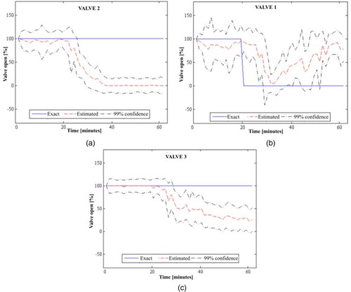
Figure 9. Exact and estimated pressure along the pipeline at the final time for configuration 2, with two measurement stations, when valve 1 was closed and the other valves were fully open.

Due to the above difficulties observed for configuration 2 when valve 1 was closed, a case was then considered with three measurement stations located at x = 9 km, x = 46 km and x = 81 km (see Figure 1b). The results obtained for the valve open percentages are presented in Figures 10a-c for this case, when valve 1 was closed while the others were fully open. The measurements taken near valve 1 provided useful information for the accurate estimation of this valve’s open percentage, as shown in Figure 10b. Similarly, valve 3 was accurately estimated as fully open because the measurements at station 2, near this valve, were mostly influenced by the outlet constant flow rate boundary condition. Such as for the case with two measurement stations, there was a trend to estimate valve 2 as closed at the final time, which was caused by the decreasing flow rate and because the pressure tended to become constant upstream of valve 1, after it was closed. However, the sudden closure of valve 1 could be accurately identified few minutes after this event, as shown in Figure 10b, but the open fraction of valve 2 gradually decreased and tended to zero only near the final time, that is, 30 minutes after the closure of valve 1 was correctly identified (see Figure 10a). Furthermore, Figures 10a and 10b show that the open percentage estimated for valve 1 was stable, but that estimated for valve 2 was oscillatory and involved large uncertainties. We note that the closure of either valve 2 or valve 3 could also be accurately identified with three measurement stations, but these results are not presented here for the sake of brevity.

Figure 10. Exact and estimated valve open percentages obtained for valve 1 closed and the other valves fully open, for configuration 2 with three measurement stations: (a) Valve 2; (b) Valve 1; (c) Valve 3.

Conclusions

This computational work dealt with the detection of the undesired and unexpected closure of automatic shutdown valves in a straight and horizontal pipeline, by solving a state estimation problem with the particle filter method. Two algorithms were compared in this work, namely: the Sampling Importance Resampling (SIR) algorithm and the Auxiliary Sampling Importance Resampling (ASIR) algorithm.

For the numerical simulations, pressure and temperature imposed at the inlet boundary were $6.5\times {10}^6\text{Pa}$ and 298 K, respectively, while the velocity imposed at the outlet boundary was 6 m/s. Simulated measurements of pressure, temperature and velocity were used for the solution of the state estimation problem. The measurements were simulated by adding Gaussian random errors to the solution of the direct problem. The standard deviations for the measurements of velocity, temperature and pressure were 0.2 m/s, 0.5 K and $2\times {10}^4\text{Pa}$, respectively. Standard deviations for the Gaussian evolution models for these state variables were assumed as twice as large, in order to account for uncertainties in the model parameters. The evolution models for the primitive flow variables resulted from the numerical solution of the compressible flow equations in the pipeline, by using a Total Variation Diminishing (TVD) Weighted Average Flux (WAF) scheme. No information was a priori assumed available for the functional form of the open fraction of each valve, which was modelled in terms of an independent Markovian process.

Both algorithms were capable of accurately identifying the sudden closure of a single valve in the middle of a pipeline with length of 90 km and diameter of 18 inch, even with the non-informative evolution model used for the valve open fraction. The ASIR algorithm with 100 particles resulted in RMS errors smaller than those of the SIR algorithm with 1000 particles. For such numbers of particles, the computational time for the ASIR algorithm was about 25% of that for the SIR algorithm. The ASIR algorithm was then applied to a configuration involving three valves in the pipeline. The closure of the valves near the two measurement stations could be accurately detected with the ASIR algorithm. On the other hand, the pressure drop resulting from the closure of the valve in the middle of the pipeline was split between the two other valves, which were then improperly predicted as closed, when the measurements of only two stations near the pipeline ends were used in the analysis. This difficulty could be alleviated by using the measurements of a third station near the valve in the middle of the pipeline, and the closure of such valve could be accurately predicted with the ASIR algorithm of the particle filter. We note that there was a trend to estimate small open fractions for valves upstream of the closed valve. This behaviour was due to the decreasing flow rate upstream of the closed valve, where the pressure tended to be constant and equal to the value assigned at the inlet boundary condition. Hence, the measurements near the pipeline inlet gradually lost sensitivity with respect to which valve was closed. On the other hand, the estimated sudden closure of the correct valve was more stable, involved smaller uncertainties and could be predicted in a shorter time than for the other upstream valves.

The ASIR algorithm of the particle filter method was shown to be an accurate quantitative technique for the detection of the undesired and unexpected closure of automatic shutdown valves in pipelines. Consequently, operators’ judgement and decision about valve closures can be kept at a minimum level. The particle filter method does not rely only on the measured data, but also on the mathematical modelling of the physical phenomena for the flow problem, and takes into account the related uncertainties.

Disclosure statement

No potential conflict of interest was reported by the author(s).

Additional information

Funding

The support provided by CNPq and FAPERJ, agencies of the Brazilian and Rio de Janeiro state governments, is gratefully appreciated. This study was financed in part by Coordenação de Aperfeiçoamento de Pessoal de Nível Superior – Brazil (CAPES) - Finance Code 001.

References

- Gato LMC, Henriques JCC. Dynamic behavior of high- pressure natural-gas flow in pipelines. Int J Heat Fluid Flow. 2005;26:816–825.
- Doucet A, De Freitas N, Gordon N. Sequential Monte Carlo methods in practice. New York: Springer; 2001; 178–195.
- Kaipio J, Somersalo E. Statistical and computational inverse problems, applied mathematical sciences 160. New York: Springer-Verlag; 2004.
- Ristic B, Arulampalam S, Gordon N. Beyond the kalman filter. Boston: Artech House; 2004.
- Arulampalam S, Maskell S, Gordon N, et al. A tutorial on particle filters for on-line non-linear/non-Gaussian Bayesian tracking. IEEE Trans Signal Processing. 2001;50:174–188.
- Robert CP, Doucet A, Andrieu C. Computational advances for and from Bayesian analysis. Stat Sci. 2004;19:118–127.
- Andrieu C, Doucet A, Singh SS, et al. Particle methods for change detection, system identification, and control. Proc IEEE. 2004;92:423–438.
- Arulampalam MS, Maskell S, Gordon N, et al. A tutorial on particle filters for online nonlinear/non-Gaussian Bayesian tracking. IEEE Trans Signal Process. 2002;50:174–188.
- Carpenter J, Clifford P, Fearnhead P. An improved particle filter for non-linear problems. IEEE Proc Radar Sonar Navig. 1999;146:2–7.
- Kantas N, Doucet A, Singh SS, et al. On particle methods for parameter estimation in state-space models. Stat. Sci. 2015;30:328–351.
- Del Moral P, Doucet A, Jasra A. Sequential Monte Carlo samplers. J R Stat Soc Ser B Stat Methodol. 2006;68:411–436.
- Lopes HF, Carvalho CM. Online Bayesian learning in dynamic models: an illustrative introduction to particle methods. In: West M, Damien P, Dellaportas P, Polson NG, Stephens DA, editors. Bayesian dynamic modelling, Bayesian inference and Markov chain Monte Carlo: In honour of Adrian Smith. Chapter 11. Oxford: Oxford University Press; 2013. DOI:https://doi.org/10.1093/acprof:oso/9780199695607.003.0011.
- Candy JV. Bayesian signal processing: classical, modern, and particle filtering methods. New York: John Wiley; 2008.
- Orlande HRB, Colaço MJ, Dulikravich GS, et al. State estimation problems in heat transfer. Int J Uncertainty Quant. 2012;2:239–258.
- Durgut I, Leblebicioglu K. Kalman-filter-based observer design around optimal control policy for gas pipelines. Int J Numer Methods Fluids. 1997;24:233–245.
- Singhal A, Salsbury TI. A simple method for detecting valve stiction in oscillating control loops. J Process Control. 2005;15:371–382.
- Horsh A, Isaksson AJ. A method for detection of stiction in control valves. In: Proceedings of the IFAC workshop on line Fault Detection and Supervision in the Chemical Process Industry, 1998.
- Lamien B, Orlande HRB, Eliçabe EG. Particle filter and approximation error model for state estimation in hyperthermia. J Heat Transfer. 2016;139:12001.
- Varon LAB, Orlande HRB, Eliçabe GE. Estimation of state variables in the hyperthermia therapy of cancer with heating imposed by radiofrequency electromagnetic waves. Int J Therm Sci. 2015;98:228–236.
- Lamien B, Orlande HRB, Eliçabe GE. Inverse problem in the hyperthermia therapy of cancer with laser heating and plasmonic nanoparticles. Inverse Probl Sci Eng. 2015;25(4):608–631.
- Varon LAB, Orlande HRB, Eliçabe GE. Combined parameter and state estimation in the radio frequency hyperthermia treatment of cancer. Numer Heat Transfer A: Appl. 2016;70:581–594.
- Lamien B, Varon LAB, Orlande HRB, et al. State estimation in bioheat transfer: a comparison of particle filter algorithms. Int J Numer Methods Heat Fluid Flow. 2017;27:615–638.
- Costa JMJ, Orlande HRB, Velho HFC, et al. Estimation of tumor size evolution using particle filters. J Comput Biol. 2015;22:150514113004000.
- Silva WB, Rochoux M, Orlande HRB, et al. Application of particle filters to regional-scale wildfire spread. High Temperatures – High Pressures. 2014;43:435–440.
- Colaço MJ, Orlande HRB, Da Silva W, et al. Application of two Bayesian filters to estimate unknown heat fluxes in a natural convection problem. J Heat Transfer. 2012;134:092501.
- Anderson J. Modern compressible flow with historical perspective. New York: McGraw-Hill; 1990.
- Anderson J. Computational fluid dynamics: The basics with applications. Singapore: McGraw-Hill; 1995.
- Herran A, De La Cruz JM, De Andres B, et al. Modeling and simulation of a gas distribution pipeline network. Appl Math Model. 2009;33:1584–1600.
- Nouri-Borujerdi A, Ziaei-Rad M. Simulation of compressible flow in high pressure buried gas pipelines. Int J Heat Mass Transf. 2009;52:5751–5758.
- Ortega AJ, Pires LFG, Nieckele AO. Una alternativa para la simulación numérica del comportamiento térmico en régimen. Información Tecnológica. 2009;20:83–88.
- Behbahani-Nejad M, Ghanbarzadeh A, Alamian R. Transient flow simulation in natural gas pipelines using the state space model. In: ASME Biennial Conference On Engineering Systems Design and Analysis, 10, 2010. Istanbul: ESDA2010, v.3,p. 409-415, 2010.
- Chaczykowski M. Transient flow in natural gas pipeline – the effect of pipeline thermal model. Applied Mathematical Modeling. 2010;34:1051–1067.
- Alamian R, Behbahani M, Ghanbarzadeh A. A state space model for transient flow simulation in natural gas pipelines. J Nat Gas Sci Eng. 2012;9:51–59.
- Bazargan-Lari MR, Kerachian R, Afshar H, et al. Developing an optimal valve closing rule curve for real-time pressure control in pipes. J Mech Sci Technol. 2013;27:215–225.
- Toro EF. Riemann solvers and numerical methods for fluid dynamics. 2nd ed. Berlin: Springer; 1999.
- Ozisik MN, Orlande HRB, Colaco M, et al. Finite difference methods in heat transfer. 2nd ed. Boca Raton: CRC Press; 2017.
- Yee HC. Numerical approximation of boundary conditions with applications to inviscid equations of gas dynamics. NASA Technical Memorandum 81265, 1981.
- Laney C. Computational gasdynamics. Cambridge: Cambridge University Press; 1998.
- Hutchison JW. ISA handbook of control valves. Research Triangle Park: Instrument Society of America – ISA; 1976.
- Baumann HD. ISA control valve primer. Research Triangle Park: ISA – International Standard Association; 2009.
- ANSI/ISA-75.02.01-2008. Control valve capacity test procedures. ISA – American National Standard, ANSI/ISA. ISBN: 978-1-936007-11-0, 2009.