Three Landweber iterative methods for solving the initial value problem of time-fractional diffusion-wave equation on spherically symmetric domain

Abstract

In this paper, the inverse problem for identifying the initial value of time-fractional diffusion wave equation on spherically symmetric region is considered. The exact solution of this problem is obtained by using the method of separating variables and the property the Mittag–Leffler functions. This problem is ill-posed, i.e. the solution(if exists) does not depend on the measurable data. Three different kinds landweber iterative methods are used to solve this problem. Under the priori and the posteriori regularization parameters choice rules, the error estimates between the exact solution and the regularization solutions are obtained. Several numerical examples are given to prove the effectiveness of these regularization methods.

Keywords:

• Time-fractional diffusion wave equation
• spherically symmetric
• Ill-posed problem
• fractional Landweber method
• inverse problem

2010 Mathematics Subject Classifications:

• 35R25
• 47A52
• 35R30

1. Introduction

Nowadays, people find that the fractional derivative has much advantages in solving practical problem, such as in medical engineering [1], chemistry and biochemistry [2], finance and economics [3–6], inverse scattering [7]. Up to now, a lot of achievements have been made in solving the direct problems [8–12] of fractional differential equations. However, when solving practical problems, the initial value, or source term, or diffusion coefficient, or part of the boundary value [13,14] is unknown, and it is necessary to invert them through some measurement data, which puts forward the inverse problem of fractional diffusion equation. The study of the fractional diffusion equation is still on an initial stage, the direct problem of it has been studied in [15–17].

For the inverse problem of time-fractional diffusion equation as $0<\alpha <1$, there are a lot of research results. For identifying the unknown source, one can see [18–26]. About backward heat conduction problem, one can see [27–34]. About identifying the initial value problem, one can see [35–37]. For an inverse unknown coefficient problem of a time-fractional equation, one can see [38,39]. About identifying the source term and initial data simultaneous of time-fractional diffusion equation, one can see [40,41]. About identifying some unknown parameters in time-fractional diffusion equation, one can see [42]. About the inverse problem for the heat equation on a columnar axis-symmetric area, one can see [43–48]. In [43–45], Landweber regularization method, a simplified Tikhonov regularization method and a spectral method are used to identify source term on a columnar axis-symmetric area. In [46–48], the authors considered a backward problem on a columnar axis-symmetric domain. In [46], Yang et al. used the quasi-boundary value regularization method to solve the inverse problem for determining the initial value of heat equation with inhomogeneous source on a columnar symmetric domain. The error estimate between the regular solution and the exact solution under the corresponding regularization parameter selection rules is obtained. Finally, numerical example is given to verify that the regularization method is very effective for solving this inverse problem. In [47], Cheng et al. used the modified Tikhonov regularization method to do with the inverse time problem for an axisymmetric heat equation. Finally, Hölder type error estimate between the approximate solution and exact solution is obtained. In [48], Djerrar et al. used standard Tikhonov regularization method to deal with an axisymmetric inverse problem for the heat equation inside the cylinder $a\le r\le b$, and numerical examples is used to show that this method is effective and stable. About the inverse problem for the time-fractional diffusion equation as $0<\alpha <1$ on a columnar and spherical symmetric areas, one can see [49,50]. In [49], Xiong proposed a backward problem model of a time-fractional diffusion-heat equation on a columnar axis-symmetric domain. Yang et al. in [50] used Landweber iterative regularization method to solve identifying the initial value of time-fractional diffusion equation on spherically symmetric domain. Compare with the inverse problem of time-fractional diffusion equation as $0<\alpha <1$, there are little research result for the inverse problem of time-fractional diffusion wave equation as $1<\alpha <2$. Šišková et al. in [51] used the regularization method to solve the inverse source problem of time-fractional diffusion wave equation. Liao et al. in [52] used conjugate gradient method combined with Morozovs discrepancy principle to identify the unknown source for the time-fractional diffusion wave equation. Šišková et al. in [53] used the regularization method to deal with an inverse source problem for a time-fractional wave equation. Gong et al. in [54] used a generalized Tikhonov to identify the time-dependent source term in a time-fractional diffusion-wave equation. In recent years, in physical oceanography and global meteorology, the inversion of initial boundary value problems has always been a hot issue. In order to increase the accuracy of numerical weather prediction, usually by the model combined with the observation data of the inversion of initial boundary value problems, and in numerical weather prediction model, provide a reasonable initial field. At present, many domestic and foreign ocean circulation model, atmospheric general circulation model, numerical weather prediction model and torrential rain forecasting model belongs to the inversion of initial boundary value problems during initialization, so such problems of scientific research application prospect is very broad. Yang et al. in [55] used the truncated regularization method to solve the inverse initial value problem of the time-fractional inhomogeneous diffusion wave equation. Yang et al. in [56] used the Landweber iterative regularization method to solve the inverse problem for identifying the initial value problem of a space time-fractional diffusion wave equation. Wei et al. in [57] used the Tikhonov regularization method to solve the inverse initial value problem of time-fractional diffusion wave equation. Wei et al. in [58] used the conjugate gradient algorithm combined with Tikhonov regularization method to identify the initial value of time-fractional diffusion wave equation. Until now, we find that there are few papers for the inverse problem of time-fractional diffusion-wave equation on a columnar axis-symmetric domain and spherically symmetric domain. In [59], the authors used the Landweber iterative method to solve an inverse source problem of time-fractional diffusion-wave equation on spherically symmetric domain. It is assumed that the grain is of a spherically symmetric domain diffusion geometry as illustrated in Figure (a-b), which is actually consistent with laboratory measurements of helium diffusion from a physical point of view from apatite. As a consequence of radiogenic production and diffusive loss, $u(r,t)$ which only depends on the spherically radius r and t denotes the concentration of helium. For the inverse problem of inversion initial value in spherically symmetric region, there are few research results at present. Whereupon, in this paper, we consider the inverse problem to identify the initial value of time-fractional diffusion-wave equation on spherically symmetric region and give three regularization methods to deal with this inverse problem in order to find a effective regular method.

In this paper, we consider the following problem: (1) $\left\{\begin{array}{ll}{D}_t^{\alpha }u(r,t)-\frac{2}{r}{u}_r(r,t)-u_{rr}(r,t)=f\left(r\right),& 0<r<r_0,0<t<T,1<\alpha <2,\\ u(r_0,t)=0,& 0\le t\le T,\\ u(r,0)=\phi \left(r\right),& 0\le r\le r_0,\\ u_t(r,0)=\psi \left(r\right),& 0\le r\le r_0,\\ \underset{r\to 0}{lim}u(r,t)bounded,& 0\le t\le T,\\ u(r,T)=g\left(r\right),& 0\le r\le r_0,\end{array}\right.$(1) where $r_0$ is the radius, $D_t^{\alpha }u(r,t)$ is the Caputo fractional derivative $(1<\alpha <2)$, it is defined as (2) $D_t^{\alpha }u(r,t)=\frac{1}{\mathrm{\Gamma }(2-\alpha )}{\int }_0^t\frac{{\mathrm{\partial }}^{2}u(r,s)}{\mathrm{\partial }{s}^2}\frac{\mathrm{d}s}{(t-s{)}^{\alpha -1}},1<\alpha <2.$(2) The existence and uniqueness of the direct problem solution has been proved in the [60]. The inverse problem is to use the measurement data $g\left(r\right)$ and the known function $f\left(r\right)$ to identify the unknown initial data $\phi \left(r\right)$, $\psi \left(r\right)$. The inverse initial value problem can be transformed into two cases:

(IVP1):	Assuming $\psi \left(r\right)$ is known, we use the final value data $g\left(r\right)$ and the known function $f\left(r\right)$ to invert the initial value $\phi \left(r\right)$.
(IVP2):	Assuming $\phi \left(r\right)$ is known, we use the final value data $g\left(r\right)$ and the known function $f\left(r\right)$ to invert the initial value $\psi \left(r\right)$.

Because the measurements are error-prone, we remark the measurements with error as $f^{\delta }$ and $g^{\delta }$ and satisfy (3) $\begin{array}{rl}& \parallel f^{\delta }-f{\parallel }_{L^2[0,r_0;r^2]}\le \delta ,\end{array}$(3) (4) $\begin{array}{rl}& \parallel g^{\delta }\left(r\right)-g\left(r\right){\parallel }_{L^2[0,r_0;r^2]}\le \delta ,\end{array}$(4) where $\delta >0$. In this paper, $L^2[0,r_0;r^2]$ represents the Hilbert space with weight $r^2$ on the interval $[0,r_0]$ of the Lebesgue measurable function. $(\cdot ,\cdot )$ and $\parallel \cdot \parallel$ represent the inner product and norm of the space of $[0,r_0;r^2]$, respectively. $\parallel \cdot \parallel$ is defined as follows: (5) $\parallel \cdot \parallel ={\left({\int }_0^{r_0}{r}^2|\cdot {|}^2\mathrm{d}r\right)}^{\frac{1}{2}}.$(5) This paper is organized as follows. In Section 2, we recall and state some preliminary theoretical results. In Section 3, we analyse the ill-posedness of the problem (IVP1) and the problem (IVP2), and give the conditional stability result. In Section 4, we give the corresponding a priori error estimates and posteriori error estimates for three regularization methods. In Section 5, we conduct some numerical tests to show the validity of the proposed regularization methods. Since most of the solutions of fractional partial differential equations contain special functions (Mittag–Leffler functions), and the calculation of these functions is quite difficult. In this paper, the difficulties are overcome through [61,62]. Finally, we give some concluding remarks.

2. Preliminary results

In this section, we give some important Lemmas.

Lemma 2.1

[57]

If $0<\alpha <2$, and $\text{β}\in \mathbb{R}$ be arbitrary. Suppose μ satisfy $\frac{\pi \alpha }{2}<\mu <min\{\pi ,\pi \alpha \}$. Then there exists a constant $C_1=C(\alpha ,\text{β},\mu )>0$ such that (6) $|E_{\alpha ,\text{β}}\left(z\right)|\le \frac{C_1}{1+|z|},\mu \le |arg\left(z\right)|\le \pi .$(6)

Lemma 2.2

[57]

For $1<\alpha <2$, $\text{β}\in \mathbb{R}$ and $\eta >0$, we have (7) $E_{\alpha ,\text{β}}(-\eta )=\frac{1}{\mathrm{\Gamma }(\text{β}-\alpha )\eta }+O\left(\frac{1}{{\eta }^2}\right),\eta \to \mathrm{\infty }.$(7)

Lemma 2.3

For $\frac{1}{2}<\gamma <1$, $a_1$ and $a_2$ are relaxation factor and satisfy $0<a_1{E}_{\alpha ,1}^2(-{\lambda }_n{T}^{\alpha })<1$, $0<a_2{T}^2{E}_{\alpha ,2}^2(-{\lambda }_n{T}^{\alpha })<1$, $m_1\ge 1$, $m_2\ge 1$, we have (8) $\begin{array}{rl}& \underset{{\lambda }_n>0}{sup}[1-(1-a_1{E}_{\alpha ,1}^2(-{\lambda }_n{T}^{\alpha }){)}^{m_1}{]}^{\gamma }\frac{1}{E_{\alpha ,1}(-{\lambda }_n{T}^{\alpha })}\le \sqrt{a_1{m}_1},\end{array}$(8) (9) $\begin{array}{rl}& \underset{{\lambda }_n>0}{sup}[1-(1-a_2{T}^2{E}_{\alpha ,2}^2(-{\lambda }_n{T}^{\alpha }){)}^{m_2}{]}^{\gamma }\frac{1}{T{E}_{\alpha ,2}(-{\lambda }_n{T}^{\alpha })}\le \sqrt{a_2{m}_2}.\end{array}$(9)

Proof.

Refer to the appendix for the details of the proof.

Lemma 2.4

For $\frac{1}{2}<\gamma <1$, $m_1\ge 1$, $m_2\ge 1$, ${\lambda }_n=(\frac{n\pi }{r_0}{)}^2>0$, $0<a_1{E}_{\alpha ,1}^2(-{\lambda }_n{T}^{\alpha })<1$, $0<a_2{T}^2{E}_{\alpha ,2}^2(-{\lambda }_n{T}^{\alpha })<1$, we have (10) $\begin{array}{rl}& \underset{{\lambda }_n>0}{sup}(1-a_1{E}_{\alpha ,1}^2(-{\lambda }_n{T}^{\alpha }\left){)}^{m_1}{E}_{\alpha ,1}^{\frac{p}{2}}\right(-{\lambda }_n{T}^{\alpha })\le c(a_1,p)m_1^{-\frac{p}{4}},\end{array}$(10) (11) $\begin{array}{rl}& \underset{{\lambda }_n>0}{sup}(1-a_2{T}^2{E}_{\alpha ,2}^2(-{\lambda }_n{T}^{\alpha }\left){)}^{m_2}{T}^{\frac{p}{2}}{E}_{\alpha ,2}^{\frac{p}{2}}\right(-{\lambda }_n{T}^{\alpha })\le c(a_2,p)m_2^{-\frac{p}{4}},\end{array}$(11) where the constant $c(a_1,p)$ is given by $c(a_1,p)=(\frac{p}{4a_1}{)}^{\frac{p}{4}}$ and $c(a_2,p)$ is given by $c(a_2,p)=(\frac{p}{4a_2}{)}^{\frac{p}{4}}$.

Proof.

Refer to the appendix for the details of the proof.

Lemma 2.5

For $1<\alpha <2$ and any fixed T>0, there is at most a finite index set $I_1=\{n_1,n_2,\dots ,n_N\}$ such that $E_{\alpha ,1}(-(\frac{n\pi }{r_0}{)}^2{T}^{\alpha })=0$ for $n\in I_1$ and $E_{\alpha ,1}(-(\frac{n\pi }{r_0}{)}^2{T}^{\alpha })\ne 0$ for $n\notin I_1$. Meanwhile there is at most a finite index set $I_2=\{m_1,m_2,\dots ,m_M\}$ such that $E_{\alpha ,2}(-(\frac{n\pi }{r_0}{)}^2{T}^{\alpha })=0$ for $n\in I_2$ and $E_{\alpha ,2}(-(\frac{n\pi }{r_0}{)}^2{T}^{\alpha })\ne 0$ for $n\notin I_2$.

Proof.

From Lemma 2.2, we know that there exists $L_0>0$ such that $E_{\alpha ,1}\left(-{\left(\frac{n\pi }{r_0}\right)}^2{T}^{\alpha }\right)\le \frac{1}{2\mathrm{\Gamma }(1-\alpha ){\left({\displaystyle \frac{n\pi }{r_0}}\right)}^2{T}^{\alpha }}<0,{\left(\frac{n\pi }{r_0}\right)}^2{T}^{\alpha }>L_0,$for $1<\alpha <2$, thus we know $E_{\alpha ,1}(-(\frac{n\pi }{r_0}{)}^2{T}^{\alpha })=0$ only if $(\frac{n\pi }{r_0}{)}^2{T}^{\alpha }\le L_0$. Since $\underset{n\to +\mathrm{\infty }}{lim}(\frac{n\pi }{r_0}{)}^2=+\mathrm{\infty }$, there are only finite $(\frac{n\pi }{r_0}{)}^2$ satisfying $(\frac{n\pi }{r_0}{)}^2{T}^{\alpha }\le L_0$. The proof for $E_{\alpha ,2}(-(\frac{n\pi }{r_0}{)}^2{T}^{\alpha })$ is similar.

Remark 2.1

The index sets $I_1$ and $I_2$ may be empty, that means the singular values for the operators $K_1$ and $K_2$ are not zeros. Here and below, all the results for $I_1=\varnothing$ and $I_2=\varnothing$ are regarded as the special cases.

Lemma 2.6

[57]

For $1<\alpha <2$ and ${\lambda }_n=(\frac{n\pi }{r_0}{)}^2$, there exists positive constants $\underset{\_}{C}$, $\overline{C}$ depending on α, T such that (12) $\begin{array}{rl}& \frac{\underset{\_}{C}}{{\lambda }_n}\le |E_{\alpha ,1}(-{\lambda }_n{T}^{\alpha })|\le \frac{\overline{C}}{{\lambda }_n},n\notin I_1,\end{array}$(12) (13) $\begin{array}{rl}& \frac{\underset{\_}{C}}{{\lambda }_n}\le |E_{\alpha ,2}(-{\lambda }_n{T}^{\alpha })|\le \frac{\overline{C}}{{\lambda }_n},n\notin I_2.\end{array}$(13)

Lemma 2.7

For $\frac{1}{2}<\gamma <1$, $m_3\ge 1$, $m_4\ge 1$, ${\lambda }_n=(\frac{n\pi }{r_0}{)}^2>0$, $0<a_1{E}_{\alpha ,1}^2(-(\frac{n\pi }{r_0}{)}^2{T}^{\alpha })<1$, $0<a_2{T}^2{E}_{\alpha ,2}^2(-(\frac{n\pi }{r_0}{)}^2{T}^{\alpha })<1$, we have (14) $\begin{array}{rl}& {\left(1-a_1{E}_{\alpha ,1}^2\left(-{\left(\frac{n\pi }{r_0}\right)}^2{T}^{\alpha }\right)\right)}^{m_3}(1+n^2{)}^{-\frac{p}{2}}\le C_3(m_3+1{)}^{-\frac{p}{4}},\end{array}$(14) (15) $\begin{array}{rl}& {\left(1-a_2{T}^2{E}_{\alpha ,2}^2\left(-{\left(\frac{n\pi }{r_0}\right)}^2{T}^{\alpha }\right)\right)}^{m_4}(1+n^2{)}^{-\frac{p}{2}}\le C_4(m_4+1{)}^{-\frac{p}{4}},\end{array}$(15) where $C_3=(\frac{a_1{\underset{\_}{C}}^2{r}_0^4}{p{\pi }^4}{)}^{-\frac{p}{4}}$ and $C_4=(\frac{a_2{T}^2{\underset{\_}{C}}^2{r}_0^4}{p{\pi }^4}{)}^{-\frac{p}{4}}$.

Proof.

Refer to the appendix for the details of the proof.

Lemma 2.8

For $\frac{1}{2}<\gamma <1$, $m_5\ge 1$, $m_6\ge 1$, ${\lambda }_n>0$, $0<a_1{E}_{\alpha ,1}^2(-(\frac{n\pi }{r_0}{)}^2{T}^{\alpha })<1$, $0<a_2{T}^2{E}_{\alpha ,2}^2(-(\frac{n\pi }{r_0}{)}^2{T}^{\alpha })<1$, we have (16) $\begin{array}{rl}& {\left(1-a_1{E}_{\alpha ,1}^{\gamma +1}\left(-{\left(\frac{n\pi }{r_0}\right)}^2{T}^{\alpha }\right)\right)}^{m_5}(1+n^2{)}^{-\frac{p}{2}}\le C_5{m}_5^{-\frac{p}{2(\gamma +1)}},\end{array}$(16) (17) $\begin{array}{rl}& {\left(1-a_2{T}^{\gamma +1}{E}_{\alpha ,2}^{\gamma +1}\left(-{\left(\frac{n\pi }{r_0}\right)}^2{T}^{\alpha }\right)\right)}^{m_6}(1+n^2{)}^{-\frac{p}{2}}\le C_6{m}_6^{-\frac{p}{2(\gamma +1)}},\end{array}$(17) where $C_5=\left(\frac{\underset{\_}{C}{r}_0^2}{{\pi }^2}{)}^{-\frac{p}{2}}\right(\frac{2a_1(\gamma +1)}{p}{)}^{-\frac{p}{2(\gamma +1)}}$ and $C_6=\left(\frac{\underset{\_}{C}T{r}_0^2}{{\pi }^2}{)}^{-\frac{p}{2}}\right(\frac{2a_2(\gamma +1)}{p}{)}^{-\frac{p}{2(\gamma +1)}}$.

Proof.

Refer to the appendix for the details of the proof.

Lemma 2.9

For $0<\gamma \le 1$, $m_5\ge 1$, $m_6\ge 1$, $0<a_1{E}_{\alpha ,1}^{\gamma +1}(-(\frac{n\pi }{r_0}{)}^2{T}^{\alpha })<1$, $0<a_2{T}^{\gamma +1}{E}_{\alpha ,2}^{\gamma +1}(-(\frac{n\pi }{r_0}{)}^2{T}^{\alpha })<1$, we have (18) $\begin{array}{rl}& \frac{1-{\left(1-a_1{E}_{\alpha ,1}^{\gamma +1}\left(-{\left({\displaystyle \frac{n\pi }{r_0}}\right)}^2{T}^{\alpha }\right)\right)}^{m_5}}{E_{\alpha ,1}\left(-{\left({\displaystyle \frac{n\pi }{r_0}}\right)}^2{T}^{\alpha }\right)}\le (a_1{m}_5{)}^{\frac{1}{\gamma +1}},\end{array}$(18) (19) $\begin{array}{rl}& \frac{1-{\left(1-a_2{T}^{\gamma +1}{E}_{\alpha ,2}^{\gamma +1}\left(-{\left({\displaystyle \frac{n\pi }{r_0}}\right)}^2{T}^{\alpha }\right)\right)}^{m_6}}{T{E}_{\alpha ,2}\left(-{\left({\displaystyle \frac{n\pi }{r_0}}\right)}^2{T}^{\alpha }\right)}\le (a_2{m}_6{)}^{\frac{1}{\gamma +1}}.\end{array}$(19)

Proof.

Refer to the appendix for the details of the proof.

Lemma 2.10

For $a_1>0$, $a_2>0$, p>0, $m_1>0$, $m_2>0$, we have (20) $\begin{array}{rl}F\left(x\right)& =\frac{\overline{C}{r}_0^2}{{\pi }^2}{\left(1-\frac{a_1{\underset{\_}{C}}^2{r}_0^4}{x^2{\pi }^4}\right)}^{m_1-1}(x{)}^{-\frac{p}{2}-1}\le C_7(m_1+1{)}^{-\frac{p+2}{4}},\end{array}$(20) (21) $\begin{array}{rl}G\left(x\right)& =\frac{T\overline{C}{r}_0^2}{{\pi }^2}{\left(1-\frac{a_2{T}^2{\underset{\_}{C}}^2{r}_0^4}{x^2{\pi }^4}\right)}^{m_2-1}(x{)}^{-\frac{p}{2}-1}\le C_8(m_2+1{)}^{-\frac{p+2}{4}},\end{array}$(21) where $C_7=\frac{\overline{C}{r}_0^2}{{\pi }^2}(\frac{a_1\underset{\_}{C}{r}_0^4}{(p+2){\pi }^4}{)}^{-\frac{p+2}{4}}$ and $C_8=\frac{T\overline{C}{r}_0^2}{{\pi }^2}(\frac{a_{2}T\underset{\_}{C}{r}_0^4}{(p+2){\pi }^4}{)}^{-\frac{p+2}{4}}$.

Proof.

Refer to the appendix for the details of the proof.

Lemma 2.11

For $a_1>0$, $a_2>0$, p>0, $m_5\ge 1$, $m_6\ge 1$, we have (22) $\begin{array}{rl}F\left(x\right)& =\frac{\overline{C}{r}_0^2}{{\pi }^2}{\left(1-a_1{\left(\frac{\underset{\_}{C}{r}_0^2}{x{\pi }^2}\right)}^{\gamma +1}\right)}^{m_5-1}(x{)}^{-\frac{p}{2}-1}\le C_9(m_5+1{)}^{-\frac{p+2}{2(\gamma +1)}},\end{array}$(22) (23) $\begin{array}{rl}G\left(x\right)& =\frac{T\overline{C}{r}_0^2}{{\pi }^2}{\left(1-a_2{T}^{\gamma +1}{\left(\frac{\underset{\_}{C}{r}_0^2}{x{\pi }^2}\right)}^{\gamma +1}\right)}^{m_6-1}(x{)}^{-\frac{p}{2}-1}\le C_{10}(m_6+1{)}^{-\frac{p+2}{2(\gamma +1)}},\end{array}$(23) where $C_9=\frac{\overline{C}{r}_0^2}{{\pi }^2}\left(\frac{\underset{\_}{C}{r}_0^2}{{\pi }^2}{)}^{-\frac{p}{2}-1}\right(\frac{a_1}{p+2}{)}^{-\frac{p+2}{2(\gamma +1)}}$ and $C_{10}=\frac{T\overline{C}{r}_0^2}{{\pi }^2}\left(\frac{T\underset{\_}{C}{r}_0^2}{{\pi }^2}{)}^{-\frac{p}{2}-1}\right(\frac{a_1}{p+2}{)}^{-\frac{p+2}{2(\gamma +1)}}$.

Proof.

Refer to the appendix for the details of the proof.

3. The ill-posedness and the conditional stability

Define (24) $H^p=\left\{f\in L^2[0,r_0;r^2];\sum _{n=1}^{\mathrm{\infty }}(1+n^2{)}^{\frac{p}{2}}(f_n,R_n\left(r\right))\right\},$(24) where $(\cdot ,\cdot )$ is the inner product in $L^2[0,r_0;r^2]$, then $H^p$ is a Hilbert space with the norm $\parallel \phi (\cdot ){\parallel }_{H^p}:=∥\sum _{n=1}^{\mathrm{\infty }}(1+n^2{)}^{\frac{p}{2}}({\phi }_n,R_n\left(r\right))∥,$and $\parallel \psi (\cdot ){\parallel }_{H^p}:=∥\sum _{n=1}^{\mathrm{\infty }}(1+n^2{)}^{\frac{p}{2}}({\psi }_n,R_n\left(r\right))∥.$

Theorem 3.1

Let $\phi \left(r\right)$, $\psi \left(r\right)\in L^2[0,r_0;r^2]$, then there exists a unique weak solution and the weak solution for (1(1) $\left\{\begin{array}{ll}{D}_t^{\alpha }u(r,t)-\frac{2}{r}{u}_r(r,t)-u_{rr}(r,t)=f\left(r\right),& 0<r<r_0,0<t<T,1<\alpha <2,\\ u(r_0,t)=0,& 0\le t\le T,\\ u(r,0)=\phi \left(r\right),& 0\le r\le r_0,\\ u_t(r,0)=\psi \left(r\right),& 0\le r\le r_0,\\ \underset{r\to 0}{lim}u(r,t)bounded,& 0\le t\le T,\\ u(r,T)=g\left(r\right),& 0\le r\le r_0,\end{array}\right.$(1) ) is given by (25) $\begin{array}{rl}u(r,t)& =\sum _{n=1}^{\mathrm{\infty }}\left[t^{\alpha -1}{E}_{\alpha ,\alpha }\left(-{\left(\frac{n\pi }{r_0}\right)}^2{t}^{\alpha }\right)\left(f\right(r),R_n(r\left)\right)\right.\\ & +E_{\alpha ,1}\left(-{\left(\frac{n\pi }{r_0}\right)}^2{t}^{\alpha }\right)\left(\phi \right(r),R_n(r\left)\right)\\ & +\left.t{E}_{\alpha ,2}\left(-{\left(\frac{n\pi }{r_0}\right)}^2{t}^{\alpha }\right)\left(\psi \right(r),R_n(r\left)\right)\right]R_n\left(r\right),\end{array}$(25) where $\left(\phi \right(r),R_n(r\left)\right)$ and $\left(\psi \right(r),R_n(r\left)\right)$ are the Fourier coefficients.

Let t = T in (25(25) $\begin{array}{rl}u(r,t)& =\sum _{n=1}^{\mathrm{\infty }}\left[t^{\alpha -1}{E}_{\alpha ,\alpha }\left(-{\left(\frac{n\pi }{r_0}\right)}^2{t}^{\alpha }\right)\left(f\right(r),R_n(r\left)\right)\right.\\ & +E_{\alpha ,1}\left(-{\left(\frac{n\pi }{r_0}\right)}^2{t}^{\alpha }\right)\left(\phi \right(r),R_n(r\left)\right)\\ & +\left.t{E}_{\alpha ,2}\left(-{\left(\frac{n\pi }{r_0}\right)}^2{t}^{\alpha }\right)\left(\psi \right(r),R_n(r\left)\right)\right]R_n\left(r\right),\end{array}$(25) ), we have $\begin{array}{rl}u(r,T)& =\sum _{n=1}^{\mathrm{\infty }}\left[T^{\alpha -1}{E}_{\alpha ,\alpha }\left(-{\left(\frac{n\pi }{r_0}\right)}^2{T}^{\alpha }\right)\left(f\right(r),R_n(r\left)\right)\right.\\ & +E_{\alpha ,1}\left(-{\left(\frac{n\pi }{r_0}\right)}^2{T}^{\alpha }\right)\left(\phi \right(r),R_n(r\left)\right)\\ & +\left.T{E}_{\alpha ,2}\left(-{\left(\frac{n\pi }{r_0}\right)}^2{T}^{\alpha }\right)\left(\psi \right(r),R_n(r\left)\right)\right]R_n\left(r\right)=g\left(r\right).\end{array}$Denote $g_1\left(r\right):=g\left(r\right)-\sum _{n=1}^{\mathrm{\infty }}\left[T^{\alpha -1}{E}_{\alpha ,\alpha }\left(-{\left(\frac{n\pi }{r_0}\right)}^2{T}^{\alpha }\right)f_n+T{E}_{\alpha ,2}\left(-{\left(\frac{n\pi }{r_0}\right)}^2{T}^{\alpha }\right){\psi }_n\right]R_n\left(r\right),$and $g_2\left(r\right):=g\left(r\right)-\sum _{n=1}^{\mathrm{\infty }}\left[T^{\alpha -1}{E}_{\alpha ,\alpha }\left(-{\left(\frac{n\pi }{r_0}\right)}^2{T}^{\alpha }\right)f_n+E_{\alpha ,1}\left(-{\left(\frac{n\pi }{r_0}\right)}^2{T}^{\alpha }\right){\phi }_n\right]R_n\left(r\right).$Then we have (26) $g_1\left(r\right)=\sum _{n=1}^{\mathrm{\infty }}{\phi }_n{E}_{\alpha ,1}\left(-{\left(\frac{n\pi }{r_0}\right)}^2{T}^{\alpha }\right)R_n\left(r\right),$(26) and (27) $g_2\left(r\right)=\sum _{n=1}^{\mathrm{\infty }}{\psi }_{n}T{E}_{\alpha ,2}\left(-{\left(\frac{n\pi }{r_0}\right)}^2{T}^{\alpha }\right)R_n\left(r\right).$(27) Now we put the definitions of ${\phi }_n$ and ${\psi }_n$ into (26(26) $g_1\left(r\right)=\sum _{n=1}^{\mathrm{\infty }}{\phi }_n{E}_{\alpha ,1}\left(-{\left(\frac{n\pi }{r_0}\right)}^2{T}^{\alpha }\right)R_n\left(r\right),$(26) ) and (27(27) $g_2\left(r\right)=\sum _{n=1}^{\mathrm{\infty }}{\psi }_{n}T{E}_{\alpha ,2}\left(-{\left(\frac{n\pi }{r_0}\right)}^2{T}^{\alpha }\right)R_n\left(r\right).$(27) ), then the problem (IVP1) and the problem (IVP2) become the following integral equations (28) $\left(K_1\phi \right)\left(\xi \right)={\int }_0^{r_0}{\kappa }_1(r,\xi )\phi \left(\xi \right)\mathrm{d}\xi =g_1\left(r\right),$(28) where the integral kernel is (29) ${\kappa }_1(r,\xi )=\sum _{n=1}^{\mathrm{\infty }}{E}_{\alpha ,1}\left(-{\left(\frac{n\pi }{r_0}\right)}^2{T}^{\alpha }\right)R_n\left(r\right)R_n\left(\xi \right).$(29) And (30) $\left(K_2\psi \right)\left(\xi \right)={\int }_0^{r_0}{\kappa }_2(r,\xi )\psi \left(\xi \right)\mathrm{d}\xi =g_2\left(r\right),$(30) where the integral kernel is (31) ${\kappa }_2(r,\xi )=\sum _{n=1}^{\mathrm{\infty }}T{E}_{\alpha ,2}\left(-{\left(\frac{n\pi }{r_0}\right)}^2{T}^{\alpha }\right)R_n\left(r\right)R_n\left(\xi \right),$(31) and due to [59], we know the linear operators $K_1$ and $K_2$ are compact from $L^2[0,r_0;r^2]$ to $L^2[0,r_0;r^2]$. The problem (IVP1) and the problem (IVP2) are ill-posed.

Let $K_1^{\ast }$ be the adjoint of $K_1$ and $K_2^{\ast }$ be the adjoint of $K_2$. Since $R_n\left(r\right)=\frac{\sqrt{2}n\pi \mathrm{s}\mathrm{i}\mathrm{n}\left(\frac{n\pi r}{r_0}\right)}{\sqrt{r_0^3}\frac{n\pi r}{r_0}}$ is a standard orthogonal system with weight $r^2$ in the $L^2[0,r_0;r^2]$, it is easy to verity $K_1^{\ast }{K}_1{R}_n\left(\xi \right)=E_{\alpha ,1}^2\left(-{\left(\frac{n\pi }{r_0}\right)}^2{T}^{\alpha }\right)R_n\left(\xi \right),$and $K_2^{\ast }{K}_2{R}_n\left(\xi \right)=T^2{E}_{\alpha ,2}^2\left(-{\left(\frac{n\pi }{r_0}\right)}^2{T}^{\alpha }\right)R_n\left(\xi \right).$Hence, the singular values of $K_1$ are ${\sigma }_{1n}^{\left(1\right)}=|E_{\alpha ,1}(-(\frac{n\pi }{r_0}{)}^2{T}^{\alpha })|$. Define (32) ${\psi }_n^{\left(1\right)}\left(r\right)=\left\{\begin{array}{ll}{R}_n\left(r\right),& E_{\alpha ,1}\left(-{\left(\frac{n\pi }{r_0}\right)}^2{T}^{\alpha }\right)\ge 0,\\ -R_n\left(r\right),& E_{\alpha ,1}\left(-{\left(\frac{n\pi }{r_0}\right)}^2{T}^{\alpha }\right)<0.\end{array}\right.$(32) It is clear that $\{{\psi }_n^{\left(1\right)}{\}}_{n=1}^{\mathrm{\infty }}$ are orthonormal in $L^2[0,r_0;r^2]$, we can verity (33) $\begin{array}{rl}& K_1{R}_n\left(\xi \right)={\sigma }_{1n}^{\left(1\right)}{\psi }_n^{\left(1\right)}\left(r\right)=E_{\alpha ,1}\left(-{\left(\frac{n\pi }{r_0}\right)}^2{T}^{\alpha }\right)R_n\left(r\right),\end{array}$(33) (34) $\begin{array}{rl}& K_1^{\ast }{\psi }_n^{\left(1\right)}\left(r\right)={\sigma }_{1n}^{\left(1\right)}{R}_n\left(\xi \right)=E_{\alpha ,1}\left(-{\left(\frac{n\pi }{r_0}\right)}^2{T}^{\alpha }\right){\psi }_n^{\left(1\right)}\left(\xi \right).\end{array}$(34) Therefore, the singular system of $K_1$ is $({\sigma }_{1n}^{\left(1\right)};R_n,{\psi }_n^{\left(1\right)})$.

By the similar verification, we know the singular system of $K_2$ is $({\sigma }_{2n}^{\left(2\right)};R_n,{\psi }_n^{\left(2\right)})$, where ${\sigma }_{2n}^{\left(2\right)}=|T{E}_{\alpha ,2}(-(\frac{n\pi }{r_0}{)}^2{T}^{\alpha })|$ and (35) ${\psi }_n^{\left(2\right)}\left(r\right)=\left\{\begin{array}{ll}{R}_n\left(r\right),& E_{\alpha ,2}\left(-{\left(\frac{n\pi }{r_0}\right)}^2{T}^{\alpha }\right)\ge 0,\\ -R_n\left(r\right),& E_{\alpha ,2}\left(-{\left(\frac{n\pi }{r_0}\right)}^2{T}^{\alpha }\right)<0.\end{array}\right.$(35) In the following, the integral kernels given in (29(29) ${\kappa }_1(r,\xi )=\sum _{n=1}^{\mathrm{\infty }}{E}_{\alpha ,1}\left(-{\left(\frac{n\pi }{r_0}\right)}^2{T}^{\alpha }\right)R_n\left(r\right)R_n\left(\xi \right).$(29) ) and (31(31) ${\kappa }_2(r,\xi )=\sum _{n=1}^{\mathrm{\infty }}T{E}_{\alpha ,2}\left(-{\left(\frac{n\pi }{r_0}\right)}^2{T}^{\alpha }\right)R_n\left(r\right)R_n\left(\xi \right),$(31) ) are rewritten as (36) $\begin{array}{rl}& {\kappa }_1(r,\xi )=\sum _{n=1,n\notin I_1}^{\mathrm{\infty }}{E}_{\alpha ,1}\left(-{\left(\frac{n\pi }{r_0}\right)}^2{T}^{\alpha }\right)R_n\left(r\right)R_n\left(\xi \right),\end{array}$(36) (37) $\begin{array}{rl}& {\kappa }_2(r,\xi )=\sum _{n=1,n\notin I_2}^{\mathrm{\infty }}T{E}_{\alpha ,2}\left(-{\left(\frac{n\pi }{r_0}\right)}^2{T}^{\alpha }\right)R_n\left(r\right)R_n\left(\xi \right).\end{array}$(37) It is not hard to prove that the kernel spaces of the operators $K_1$ and $K_2$ are $\begin{array}{rl}& N\left(K_1\right)=\mathrm{s}\mathrm{p}\mathrm{a}\mathrm{n}\{R_n;n\in I_1\}\mathrm{f}\mathrm{o}\mathrm{r}{I}_1\ne \varnothing ;N\left(K_1\right)=\left\{0\right\}\mathrm{f}\mathrm{o}\mathrm{r}{I}_1=\varnothing ,\\ & N\left(K_2\right)=\mathrm{s}\mathrm{p}\mathrm{a}\mathrm{n}\{R_n;n\in I_2\}\mathrm{f}\mathrm{o}\mathrm{r}{I}_2\ne \varnothing ;N\left(K_2\right)=\left\{0\right\}\mathrm{f}\mathrm{o}\mathrm{r}{I}_2=\varnothing ,\end{array}$and the ranges of the operators $K_1$ and $K_2$ are $\begin{array}{rl}R\left(K_1\right)& =\left\{\phantom{{\left(\frac{(g_1,R_n)}{E_{\alpha ,1}\left(-{\left({\displaystyle \frac{n\pi }{r_0}}\right)}^2{T}^{\alpha }\right)}\right)}^2}{g}_1\in L^2[0,r_0;r^2]|(g_1,R_n)=0,n\notin I_1;\right.\\ & \left.\sum _{n=1,n\notin I_1}^{\mathrm{\infty }}{\left(\frac{(g_1,R_n)}{E_{\alpha ,1}\left(-{\left({\displaystyle \frac{n\pi }{r_0}}\right)}^2{T}^{\alpha }\right)}\right)}^2<+\mathrm{\infty }\right\},\\ R\left(K_2\right)& =\left\{\phantom{{\left(\frac{(g_1,R_n)}{E_{\alpha ,1}\left(-{\left({\displaystyle \frac{n\pi }{r_0}}\right)}^2{T}^{\alpha }\right)}\right)}^2}{g}_2\in L^2[0,r_0;r^2]|(g_2,R_n)=0,n\notin I_2;\right.\\ & \left.\sum _{n=1,n\notin I_2}^{\mathrm{\infty }}{\left(\frac{(g_2,R_n)}{T{E}_{\alpha ,2}\left(-{\left({\displaystyle \frac{n\pi }{r_0}}\right)}^2{T}^{\alpha }\right)}\right)}^2<+\mathrm{\infty }\right\}.\end{array}$Therefore, we have the following existence of the solutions for the integral equations:

Theorem 3.2

If $I_1=\varnothing$, for any $g_1\in R\left(K_1\right)$, there exists a unique solution in $L^2[0,r_0;r^2]$ for the integral Equation  (28(28) $\left(K_1\phi \right)\left(\xi \right)={\int }_0^{r_0}{\kappa }_1(r,\xi )\phi \left(\xi \right)\mathrm{d}\xi =g_1\left(r\right),$(28) ) given by (38) $\phi \left(r\right)=\sum _{n=1}^{\mathrm{\infty }}\frac{g_{1n}}{E_{\alpha ,1}\left(-{\left({\displaystyle \frac{n\pi }{r_0}}\right)}^2{T}^{\alpha }\right)}{R}_n\left(r\right).$(38) If $I_1\ne \varnothing$, for any $g_1\in R\left(K_1\right)$, there exists infinitely many solutions for the integral equation  (28(28) $\left(K_1\phi \right)\left(\xi \right)={\int }_0^{r_0}{\kappa }_1(r,\xi )\phi \left(\xi \right)\mathrm{d}\xi =g_1\left(r\right),$(28) ) , but exists only one best approximate solution in $L^2[0,r_0;r^2]$ as (39) $\phi \left(r\right)=\sum _{n=1,n\notin I_1}^{\mathrm{\infty }}\frac{g_{1n}}{E_{\alpha ,1}\left(-{\left({\displaystyle \frac{n\pi }{r_0}}\right)}^2{T}^{\alpha }\right)}{R}_n\left(r\right).$(39)

Proof.

Suppose $\phi \left(\xi \right)=\sum _{n=1}^{\mathrm{\infty }}{\phi }_n{R}_n\left(\xi \right)$, put $g_1=\sum _{n=1,n\notin I_1}^{\mathrm{\infty }}{g}_{1n}{R}_n\left(r\right)$ into (28(28) $\left(K_1\phi \right)\left(\xi \right)={\int }_0^{r_0}{\kappa }_1(r,\xi )\phi \left(\xi \right)\mathrm{d}\xi =g_1\left(r\right),$(28) ), according to the orthonormality of $\left\{R_n\right\}$, it is not hard to obtain the results.

Theorem 3.3

If $I_2=\varnothing$, for any $g_2\in R\left(K_2\right)$, there exists a unique solution in $L^2[0,r_0;r^2]$ for the integral equation  (30(30) $\left(K_2\psi \right)\left(\xi \right)={\int }_0^{r_0}{\kappa }_2(r,\xi )\psi \left(\xi \right)\mathrm{d}\xi =g_2\left(r\right),$(30) ) given by (40) $\psi \left(r\right)=\sum _{n=1}^{\mathrm{\infty }}\frac{g_{2n}}{T{E}_{\alpha ,2}\left(-{\left({\displaystyle \frac{n\pi }{r_0}}\right)}^2{T}^{\alpha }\right)}{R}_n\left(r\right).$(40) If $I_2\ne \varnothing$, for any $g_2\in R\left(K_2\right)$, there exists infinitely many solutions for the integral equation  (30(30) $\left(K_2\psi \right)\left(\xi \right)={\int }_0^{r_0}{\kappa }_2(r,\xi )\psi \left(\xi \right)\mathrm{d}\xi =g_2\left(r\right),$(30) ) , but exists only one best approximate solution as (41) $\psi \left(r\right)=\sum _{n=1,n\notin I_2}^{\mathrm{\infty }}\frac{g_{2n}}{T{E}_{\alpha ,2}\left(-{\left({\displaystyle \frac{n\pi }{r_0}}\right)}^2{T}^{\alpha }\right)}{R}_n\left(r\right).$(41)

Proof.

The proof is similar to the Theorem 3.2.

We have the following theorem on conditional stability:

Theorem 3.4

When $\phi \left(r\right)$ satisfies the a-priori bound condition (42) $\parallel \phi \left(r\right){\parallel }_{H^p}\le E_1,p>0,$(42) where $E_1$ and p are positive constants, we have (43) $\parallel \phi \left(r\right)\parallel \le C_{11}{E}_1^{\frac{2}{p+2}}\parallel g_1{\parallel }^{\frac{p}{p+2}},$(43) where $C_{11}=(\frac{{\pi }^2}{\underset{\_}{C}{r}_0^2}{)}^{\frac{p}{p+2}}$ is a constant.

Proof.

Due to (39(39) $\phi \left(r\right)=\sum _{n=1,n\notin I_1}^{\mathrm{\infty }}\frac{g_{1n}}{E_{\alpha ,1}\left(-{\left({\displaystyle \frac{n\pi }{r_0}}\right)}^2{T}^{\alpha }\right)}{R}_n\left(r\right).$(39) ) and H$\ddot{o}$lder inequality, we have (44) $\begin{array}{rl}\parallel \phi \left(r\right){\parallel }^2& =\sum _{n=1,n\notin I_1}^{\mathrm{\infty }}{\phi }_n^2=\sum _{n=1,n\notin I_1}^{\mathrm{\infty }}\frac{g_{1n}^2}{E_{\alpha ,1}^2\left(-{\left({\displaystyle \frac{n\pi }{r_0}}\right)}^2{T}^{\alpha }\right)}\\ & =\sum _{n=1,n\notin I_1}^{\mathrm{\infty }}\frac{g_{1n}^{\frac{4}{p+2}}}{E_{\alpha ,1}^2\left(-{\left({\displaystyle \frac{n\pi }{r_0}}\right)}^2{T}^{\alpha }\right)}{g}_{1n}^{\frac{2p}{p+2}}\\ & \le {\left(\sum _{n=1,n\notin I_1}^{\mathrm{\infty }}\frac{g_{1n}^2}{E_{\alpha ,1}^{p+2}\left(-{\left({\displaystyle \frac{n\pi }{r_0}}\right)}^2{T}^{\alpha }\right)}\right)}^{\frac{2}{p+2}}{\left(\sum _{n=1,n\notin I_1}^{\mathrm{\infty }}{g}_{1n}^2\right)}^{\frac{p}{p+2}}.\end{array}$(44) Applying Lemma 2.6 and (39(39) $\phi \left(r\right)=\sum _{n=1,n\notin I_1}^{\mathrm{\infty }}\frac{g_{1n}}{E_{\alpha ,1}\left(-{\left({\displaystyle \frac{n\pi }{r_0}}\right)}^2{T}^{\alpha }\right)}{R}_n\left(r\right).$(39) ), we obtain (45) $\begin{array}{rl}\sum _{n=1,n\notin I_1}^{\mathrm{\infty }}\frac{g_{1n}^2}{E_{\alpha ,1}^{p+2}\left(-{\left({\displaystyle \frac{n\pi }{r_0}}\right)}^2{T}^{\alpha }\right)}& \le \sum _{n=1,n\notin I_1}^{\mathrm{\infty }}\frac{g_{1n}^2}{E_{\alpha ,1}^2\left(-{\left({\displaystyle \frac{n\pi }{r_0}}\right)}^2{T}^{\alpha }\right)}{\left(\frac{{\lambda }_n}{\underset{\_}{C}}\right)}^p\\ & =\sum _{n=1,n\notin I_1}^{\mathrm{\infty }}{\phi }_n^2{\left(\frac{n^2{\pi }^2}{\underset{\_}{C}{r}_0^2}\right)}^p\\ & \le \sum _{n=1,n\notin I_1}^{\mathrm{\infty }}{\left(\frac{{\pi }^2}{\underset{\_}{C}{r}_0^2}\right)}^p\parallel \phi {\parallel }_{H^p}^2.\end{array}$(45) Combining (44(44) $\begin{array}{rl}\parallel \phi \left(r\right){\parallel }^2& =\sum _{n=1,n\notin I_1}^{\mathrm{\infty }}{\phi }_n^2=\sum _{n=1,n\notin I_1}^{\mathrm{\infty }}\frac{g_{1n}^2}{E_{\alpha ,1}^2\left(-{\left({\displaystyle \frac{n\pi }{r_0}}\right)}^2{T}^{\alpha }\right)}\\ & =\sum _{n=1,n\notin I_1}^{\mathrm{\infty }}\frac{g_{1n}^{\frac{4}{p+2}}}{E_{\alpha ,1}^2\left(-{\left({\displaystyle \frac{n\pi }{r_0}}\right)}^2{T}^{\alpha }\right)}{g}_{1n}^{\frac{2p}{p+2}}\\ & \le {\left(\sum _{n=1,n\notin I_1}^{\mathrm{\infty }}\frac{g_{1n}^2}{E_{\alpha ,1}^{p+2}\left(-{\left({\displaystyle \frac{n\pi }{r_0}}\right)}^2{T}^{\alpha }\right)}\right)}^{\frac{2}{p+2}}{\left(\sum _{n=1,n\notin I_1}^{\mathrm{\infty }}{g}_{1n}^2\right)}^{\frac{p}{p+2}}.\end{array}$(44) ) and (45(45) $\begin{array}{rl}\sum _{n=1,n\notin I_1}^{\mathrm{\infty }}\frac{g_{1n}^2}{E_{\alpha ,1}^{p+2}\left(-{\left({\displaystyle \frac{n\pi }{r_0}}\right)}^2{T}^{\alpha }\right)}& \le \sum _{n=1,n\notin I_1}^{\mathrm{\infty }}\frac{g_{1n}^2}{E_{\alpha ,1}^2\left(-{\left({\displaystyle \frac{n\pi }{r_0}}\right)}^2{T}^{\alpha }\right)}{\left(\frac{{\lambda }_n}{\underset{\_}{C}}\right)}^p\\ & =\sum _{n=1,n\notin I_1}^{\mathrm{\infty }}{\phi }_n^2{\left(\frac{n^2{\pi }^2}{\underset{\_}{C}{r}_0^2}\right)}^p\\ & \le \sum _{n=1,n\notin I_1}^{\mathrm{\infty }}{\left(\frac{{\pi }^2}{\underset{\_}{C}{r}_0^2}\right)}^p\parallel \phi {\parallel }_{H^p}^2.\end{array}$(45) ), we can get $\parallel \phi \left(r\right)\parallel \le C_{11}\parallel \phi {\parallel }_{H^p}^{\frac{2}{p+2}}\parallel g_1{\parallel }^{\frac{p}{p+2}}.\text{■}$

Theorem 3.5

As $\psi \left(r\right)$ satisfies a-priori bound condition (46) $\parallel \psi \left(r\right){\parallel }_{H^p}\le E_2,p>0,$(46) where $E_2$ and p are positive constants, then (47) $\parallel \psi \left(r\right)\parallel \le C_{12}{E}_2^{\frac{2}{p+2}}\parallel g_2{\parallel }^{\frac{p}{p+2}},$(47) where $C_{12}=(\frac{{\pi }^2}{T\underset{\_}{C}{r}_0^2}{)}^{\frac{p}{p+2}}$ is a constant.

Proof.

The proof is similar to the Theorem 3.4, so it is omitted.

4. Regularization method and error estimation

By referring to [59,64,65], we find a classical Landweber regularization method and two fractional Landweber iterative regularization methods, but it has not been explained which of these methods is better. So, in this section, we mainly make use of two kinds of fractional Landweber regularization methods and the classical Landweber regularization method to solve the problem (IVP1) and the problem (IVP2). The error estimates between the exact solution and the corresponding regular solution are given, respectively. By using three regularization methods to solve the same problem, an optimal regularization method is obtained.

By [64], the fractional Landweber regularization solution is given as follows: (48) ${\phi }^{m_1,\delta }=\sum _{n=1,n\notin I_1}^{\mathrm{\infty }}\frac{{\left[1-{\left(1-a_1{E}_{\alpha ,1}^2\left(-{\left({\displaystyle \frac{n\pi }{r_0}}\right)}^2{T}^{\alpha }\right)\right)}^{m_1}\right]}^{\gamma }}{E_{\alpha ,1}\left(-{\left({\displaystyle \frac{n\pi }{r_0}}\right)}^2{T}^{\alpha }\right)}{g}_{1n}^{\delta }{R}_n\left(r\right),$(48) and (49) ${\psi }^{m_2,\delta }=\sum _{n=1,n\notin I_2}^{\mathrm{\infty }}\frac{{\left[1-{\left(1-a_2{T}^2{E}_{\alpha ,2}^2\left(-{\left({\displaystyle \frac{n\pi }{r_0}}\right)}^2{T}^{\alpha }\right)\right)}^{m_2}\right]}^{\gamma }}{T{E}_{\alpha ,2}\left(-{\left({\displaystyle \frac{n\pi }{r_0}}\right)}^2{T}^{\alpha }\right)}{g}_{2n}^{\delta }{R}_n\left(r\right).$(49) By [59], the Landweber regularization solution is given as follows: (50) ${\phi }^{m_3,\delta }=\sum _{n=1,n\notin I_1}^{\mathrm{\infty }}\frac{1-{\left(1-a_1{E}_{\alpha ,1}^2\left(-{\left({\displaystyle \frac{n\pi }{r_0}}\right)}^2{T}^{\alpha }\right)\right)}^{m_3}}{E_{\alpha ,1}\left(-{\left({\displaystyle \frac{n\pi }{r_0}}\right)}^2{T}^{\alpha }\right)}{g}_{1n}^{\delta }{R}_n\left(r\right),$(50) and (51) ${\psi }^{m_4,\delta }=\sum _{n=1,n\notin I_2}^{\mathrm{\infty }}\frac{1-{\left(1-a_2{T}^2{E}_{\alpha ,2}^2\left(-{\left({\displaystyle \frac{n\pi }{r_0}}\right)}^2{T}^{\alpha }\right)\right)}^{m_4}}{T{E}_{\alpha ,2}\left(-{\left({\displaystyle \frac{n\pi }{r_0}}\right)}^2{T}^{\alpha }\right)}{g}_{2n}^{\delta }{R}_n\left(r\right).$(51) By [65], the modified iterative regularization solution is given as follows: (52) ${\phi }^{m_5,\delta }=\sum _{n=1,n\notin I_1}^{\mathrm{\infty }}\frac{1-{\left(1-a_1{E}_{\alpha ,1}^{\gamma +1}\left(-{\left({\displaystyle \frac{n\pi }{r_0}}\right)}^2{T}^{\alpha }\right)\right)}^{m_5}}{E_{\alpha ,1}\left(-{\left({\displaystyle \frac{n\pi }{r_0}}\right)}^2{T}^{\alpha }\right)}{g}_{1n}^{\delta }{R}_n\left(r\right),$(52) and (53) ${\psi }^{m_6,\delta }=\sum _{n=1,n\notin I_2}^{\mathrm{\infty }}\frac{1-{\left(1-a_2{T}^{\gamma +1}{E}_{\alpha ,2}^{\gamma +1}\left(-{\left({\displaystyle \frac{n\pi }{r_0}}\right)}^2{T}^{\alpha }\right)\right)}^{m_6}}{T{E}_{\alpha ,2}\left(-{\left({\displaystyle \frac{n\pi }{r_0}}\right)}^2{T}^{\alpha }\right)}{g}_{2n}^{\delta }{R}_n\left(r\right),$(53) where $a_1$, $a_2$ are relaxation factors and satisfy $a_1$, $a_2>0$, $\frac{1}{2}<\gamma \le 1$.

4.1. The priori error estimate

Lemma 4.1

Suppose $f\left(x\right)$ and $g\left(x\right)$ be $\in L^2(0,r_0;r^2)$, there is a constant ${\mathbb{M}}_1$ to make: $\begin{array}{rl}\mathbb{Q}\left(r\right)& =\parallel g\left(r\right)-\sum _{n=1}^{\mathrm{\infty }}\left[T^{\alpha -1}{E}_{\alpha ,\alpha }\left(-{\left(\frac{n\pi }{r_0}\right)}^2{T}^{\alpha }\right)f_n\right]R_n\left(r\right)\parallel \\ & \le \sqrt{2[\parallel g{\parallel }_{L^2[0,r_0;r^2]}^2+{\mathbb{M}}_1^2\parallel f{\parallel }_{L^2[0,r_0;r^2]}^2]},\end{array}$where ${\mathbb{M}}_1=\frac{C_1{r}_0^2}{n^2{\pi }^{2}T}$.

Proof.

From Lemma 2.1, we have $E_{\alpha ,\alpha }\left(-{\left(\frac{n\pi }{r_0}\right)}^2{T}^{\alpha }\right)\le \frac{C_1}{{\left({\displaystyle \frac{n\pi }{r_0}}\right)}^2{T}^{\alpha }}=\frac{C_1{r}_0^2}{n^2{\pi }^2{T}^{\alpha }}.$Thus, $\begin{array}{rl}\parallel \mathbb{Q}\left(r\right){\parallel }^2& =\parallel g\left(r\right)-\sum _{n=1}^{\mathrm{\infty }}\left[T^{\alpha -1}{E}_{\alpha ,\alpha }\left(-{\left(\frac{n\pi }{r_0}\right)}^2{T}^{\alpha }\right)f_n\right]R_n\left(r\right){\parallel }^2\\ & =\sum _{n=1}^{\mathrm{\infty }}{\left(g_n-T^{\alpha -1}{E}_{\alpha ,\alpha }\left(-{\left(\frac{n\pi }{r_0}\right)}^2{T}^{\alpha }\right)f_n\right)}^2\\ & \le 2\sum _{n=1}^{\mathrm{\infty }}{g}_n^2+2T^{2\alpha -2}{E}_{\alpha ,\alpha }^2\left(-{\left(\frac{n\pi }{r_0}\right)}^2{T}^{\alpha }\right)\sum _{n=1}^{\mathrm{\infty }}{f}_n^2\\ & \le 2[\parallel g{\parallel }_{L^2[0,r_0;r^2]}^2+{\mathbb{M}}_1^2\parallel f{\parallel }_{L^2[0,r_0;r^2]}^2],\end{array}$where ${\mathbb{M}}_1=\frac{C_1{r}_0^2}{n^2{\pi }^{2}T}$. We complete the proof of Lemma 4.1.

Remark 4.1

Suppose ${\mathbb{Q}}^{\delta }\left(r\right)=∥g^{\delta }\left(r\right)-\sum _{n=1}^{\mathrm{\infty }}\left[T^{\alpha -1}{E}_{\alpha ,\alpha }\left(-{\left(\frac{n\pi }{r_0}\right)}^2{T}^{\alpha }\right)f_n^{\delta }\right]R_n\left(r\right)∥.$From Lemma 4.1, (3(3) $\begin{array}{rl}& \parallel f^{\delta }-f{\parallel }_{L^2[0,r_0;r^2]}\le \delta ,\end{array}$(3) ) and (4(4) $\begin{array}{rl}& \parallel g^{\delta }\left(r\right)-g\left(r\right){\parallel }_{L^2[0,r_0;r^2]}\le \delta ,\end{array}$(4) ), we easily know $\parallel \mathbb{Q}\left(r\right)-{\mathbb{Q}}^{\delta }\left(r\right)\parallel \le \sqrt{2({\mathbb{M}}_1^2+1)}\delta$.

Define an orthogonal projection operator ${\mathcal{Q}}_1:L^2[0,r_0;r^2]\to \overline{R\left(K_1\right)}$, combining Equations (3(3) $\begin{array}{rl}& \parallel f^{\delta }-f{\parallel }_{L^2[0,r_0;r^2]}\le \delta ,\end{array}$(3) ) and (4(4) $\begin{array}{rl}& \parallel g^{\delta }\left(r\right)-g\left(r\right){\parallel }_{L^2[0,r_0;r^2]}\le \delta ,\end{array}$(4) ), we have: $\parallel {\mathcal{Q}}_1{g}_1^{\delta }-{\mathcal{Q}}_1{g}_1\parallel \le \parallel g_1^{\delta }-g_1\parallel =\parallel g^{\delta }-g\parallel \le \sqrt{2({\mathbb{M}}_1^2+1)}\delta .$Define an orthogonal projection operator ${\mathcal{Q}}_2:L^2[0,r_0;r^2]\to \overline{R\left(K_2\right)}$, combining Equations (3(3) $\begin{array}{rl}& \parallel f^{\delta }-f{\parallel }_{L^2[0,r_0;r^2]}\le \delta ,\end{array}$(3) ) and (4(4) $\begin{array}{rl}& \parallel g^{\delta }\left(r\right)-g\left(r\right){\parallel }_{L^2[0,r_0;r^2]}\le \delta ,\end{array}$(4) ), we have: $\parallel {\mathcal{Q}}_2{g}_2^{\delta }-{\mathcal{Q}}_2{g}_2\parallel \le \parallel g_2^{\delta }-g_2\parallel =\parallel g^{\delta }-g\parallel \le \sqrt{2({\mathbb{M}}_1^2+1)}\delta .$

Theorem 4.1

Let $m_1=\left[\right(\frac{E_1}{\delta }{)}^{\frac{4}{p+2}}]$. If the a-priori condition  (42(42) $\parallel \phi \left(r\right){\parallel }_{H^p}\le E_1,p>0,$(42) ) and Lemma  4.1 hold, we have the following convergence estimate (54) $\parallel {\phi }^{m_1,\delta }\left(r\right)-\phi \left(r\right)\parallel \le C_{13}{E}_1^{\frac{2}{p+2}}{\delta }^{\frac{p}{p+2}},$(54) where $C_{13}=c(a_1,p)(\frac{\underset{\_}{C}{r}_0^2}{{\pi }^2}{)}^{-\frac{p}{2}}+\sqrt{2a_1({\mathbb{M}}_1^2+1)}$, and $\left[x\right]$ denotes the largest integer smaller than or equal to x.

Proof.

Using the triangle inequality, we have $\parallel {\phi }^{m_1,\delta }\left(r\right)-\phi \left(r\right)\parallel \le \parallel {\phi }^{m_1,\delta }\left(r\right)-{\phi }^{m_1}\left(r\right)\parallel +\parallel \phi \left(r\right)-{\phi }^{m_1}\left(r\right)\parallel =I_1+I_2.$From (8(8) $\begin{array}{rl}& \underset{{\lambda }_n>0}{sup}[1-(1-a_1{E}_{\alpha ,1}^2(-{\lambda }_n{T}^{\alpha }){)}^{m_1}{]}^{\gamma }\frac{1}{E_{\alpha ,1}(-{\lambda }_n{T}^{\alpha })}\le \sqrt{a_1{m}_1},\end{array}$(8) ) and Remark 4.1, we have $\begin{array}{rl}{I}_1^2& =\parallel {\phi }^{m_1,\delta }\left(r\right)-{\phi }^{m_1}\left(r\right){\parallel }^2\\ & ={∥\sum _{n=1,n\notin I_1}^{\mathrm{\infty }}\frac{{\left[1-{\left(1-a_1{E}_{\alpha ,1}^2\left(-{\left({\displaystyle \frac{n\pi }{r_0}}\right)}^2{T}^{\alpha }\right)\right)}^{m_1}\right]}^{\gamma }}{E_{\alpha ,1}\left(-{\left({\displaystyle \frac{n\pi }{r_0}}\right)}^2{T}^{\alpha }\right)}(g_{1n}^{\delta }-g_{1n})R_n\left(r\right)∥}^2\\ & \le \underset{n\ge 1,n\notin I_1}{sup}\frac{{\left[1-{\left(1-a_1{E}_{\alpha ,1}^2\left(-{\left({\displaystyle \frac{n\pi }{r_0}}\right)}^2{T}^{\alpha }\right)\right)}^{m_1}\right]}^{2\gamma }}{E_{\alpha ,1}^2\left(-{\left({\displaystyle \frac{n\pi }{r_0}}\right)}^2{T}^{\alpha }\right)}\sum _{n=1,n\notin I_1}^{\mathrm{\infty }}(g_{1n}^{\delta }-g_{1n}{)}^2\\ & \le 2a_1{m}_1({\mathbb{M}}_1^2+1){\delta }^2.\end{array}$Then we can get (55) $\parallel {\phi }^{m_1,\delta }\left(r\right)-{\phi }^{m_1}\left(r\right)\parallel \le \sqrt{2a_1{m}_1({\mathbb{M}}_1^2+1)}\delta .$(55) For the second part, (56) $\begin{array}{rl}{I}_2^2& =\parallel \phi \left(r\right)-{\phi }^{m_1}\left(r\right){\parallel }^2\\ & ={∥\sum _{n=1,n\notin I_1}^{\mathrm{\infty }}\frac{1-{\left[1-{\left(1-a_1{E}_{\alpha ,1}^2\left(-{\left({\displaystyle \frac{n\pi }{r_0}}\right)}^2{T}^{\alpha }\right)\right)}^{m_1}\right]}^{\gamma }}{E_{\alpha ,1}\left(-{\left({\displaystyle \frac{n\pi }{r_0}}\right)}^2{T}^{\alpha }\right)}{g}_{1n}{R}_n\left(r\right)∥}^2\\ & \le {∥\sum _{n=1,n\notin I_1}^{\mathrm{\infty }}\frac{{\left(1-a_1{E}_{\alpha ,1}^2\left(-{\left({\displaystyle \frac{n\pi }{r_0}}\right)}^2{T}^{\alpha }\right)\right)}^{m_1}}{E_{\alpha ,1}\left(-{\left({\displaystyle \frac{n\pi }{r_0}}\right)}^2{T}^{\alpha }\right)}{g}_{1n}{R}_n\left(r\right)∥}^2\\ & =\sum _{n=1,n\notin I_1}^{\mathrm{\infty }}\frac{{\left(1-a_1{E}_{\alpha ,1}^2\left(-{\left({\displaystyle \frac{n\pi }{r_0}}\right)}^2{T}^{\alpha }\right)\right)}^{2m_1}}{E_{\alpha ,1}^2\left(-{\left({\displaystyle \frac{n\pi }{r_0}}\right)}^2{T}^{\alpha }\right)}{g}_{1n}^2\\ & =\sum _{n=1,n\notin I_1}^{\mathrm{\infty }}{\left(1-a_1{E}_{\alpha ,1}^2\left(-{\left(\frac{n\pi }{r_0}\right)}^2{T}^{\alpha }\right)\right)}^{2m_1}{\phi }_n^2\left(r\right)\\ & =\sum _{n=1,n\notin I_1}^{\mathrm{\infty }}{\left(1-a_1{E}_{\alpha ,1}^2\left(-{\left(\frac{n\pi }{r_0}\right)}^2{T}^{\alpha }\right)\right)}^{2m_1}(1+n^2{)}^{-p}(1+n^2{)}^p{\phi }_n^2\left(r\right)\\ & \le E_1^2\underset{n\ge 1}{sup}\left(B\right(n){)}^2,\end{array}$(56) where $B\left(n\right):=(1-a_1{E}_{\alpha ,1}^2(-\left(\frac{n\pi }{r_0}{)}^2{T}^{\alpha }\right){)}^{m_1}(1+n^2{)}^{-\frac{p}{2}}$.

From (10(10) $\begin{array}{rl}& \underset{{\lambda }_n>0}{sup}(1-a_1{E}_{\alpha ,1}^2(-{\lambda }_n{T}^{\alpha }\left){)}^{m_1}{E}_{\alpha ,1}^{\frac{p}{2}}\right(-{\lambda }_n{T}^{\alpha })\le c(a_1,p)m_1^{-\frac{p}{4}},\end{array}$(10) ), we have (57) $\begin{array}{rl}B\left(n\right)& \le {\left(1-a_1{E}_{\alpha ,1}^2\left(-{\left(\frac{n\pi }{r_0}\right)}^2{T}^{\alpha }\right)\right)}^{m_1}(n^2{)}^{-\frac{p}{2}}\\ & \le {\left(1-a_1{E}_{\alpha ,1}^2\left(-{\left(\frac{n\pi }{r_0}\right)}^2{T}^{\alpha }\right)\right)}^{m_1}{\left(\frac{\underset{\_}{C}{r}_0^2}{{\pi }^2}\right)}^{-\frac{p}{2}}{E}_{\alpha ,1}^{\frac{p}{2}}\left(-{\left(\frac{n\pi }{r_0}\right)}^2{T}^{\alpha }\right)\\ & \le {\left(\frac{\underset{\_}{C}{r}_0^2}{{\pi }^2}\right)}^{-\frac{p}{2}}c(a_1,p)m_1^{-\frac{p}{4}}.\end{array}$(57) Combining (55(55) $\parallel {\phi }^{m_1,\delta }\left(r\right)-{\phi }^{m_1}\left(r\right)\parallel \le \sqrt{2a_1{m}_1({\mathbb{M}}_1^2+1)}\delta .$(55) ), (56(56) $\begin{array}{rl}{I}_2^2& =\parallel \phi \left(r\right)-{\phi }^{m_1}\left(r\right){\parallel }^2\\ & ={∥\sum _{n=1,n\notin I_1}^{\mathrm{\infty }}\frac{1-{\left[1-{\left(1-a_1{E}_{\alpha ,1}^2\left(-{\left({\displaystyle \frac{n\pi }{r_0}}\right)}^2{T}^{\alpha }\right)\right)}^{m_1}\right]}^{\gamma }}{E_{\alpha ,1}\left(-{\left({\displaystyle \frac{n\pi }{r_0}}\right)}^2{T}^{\alpha }\right)}{g}_{1n}{R}_n\left(r\right)∥}^2\\ & \le {∥\sum _{n=1,n\notin I_1}^{\mathrm{\infty }}\frac{{\left(1-a_1{E}_{\alpha ,1}^2\left(-{\left({\displaystyle \frac{n\pi }{r_0}}\right)}^2{T}^{\alpha }\right)\right)}^{m_1}}{E_{\alpha ,1}\left(-{\left({\displaystyle \frac{n\pi }{r_0}}\right)}^2{T}^{\alpha }\right)}{g}_{1n}{R}_n\left(r\right)∥}^2\\ & =\sum _{n=1,n\notin I_1}^{\mathrm{\infty }}\frac{{\left(1-a_1{E}_{\alpha ,1}^2\left(-{\left({\displaystyle \frac{n\pi }{r_0}}\right)}^2{T}^{\alpha }\right)\right)}^{2m_1}}{E_{\alpha ,1}^2\left(-{\left({\displaystyle \frac{n\pi }{r_0}}\right)}^2{T}^{\alpha }\right)}{g}_{1n}^2\\ & =\sum _{n=1,n\notin I_1}^{\mathrm{\infty }}{\left(1-a_1{E}_{\alpha ,1}^2\left(-{\left(\frac{n\pi }{r_0}\right)}^2{T}^{\alpha }\right)\right)}^{2m_1}{\phi }_n^2\left(r\right)\\ & =\sum _{n=1,n\notin I_1}^{\mathrm{\infty }}{\left(1-a_1{E}_{\alpha ,1}^2\left(-{\left(\frac{n\pi }{r_0}\right)}^2{T}^{\alpha }\right)\right)}^{2m_1}(1+n^2{)}^{-p}(1+n^2{)}^p{\phi }_n^2\left(r\right)\\ & \le E_1^2\underset{n\ge 1}{sup}\left(B\right(n){)}^2,\end{array}$(56) ) and (57(57) $\begin{array}{rl}B\left(n\right)& \le {\left(1-a_1{E}_{\alpha ,1}^2\left(-{\left(\frac{n\pi }{r_0}\right)}^2{T}^{\alpha }\right)\right)}^{m_1}(n^2{)}^{-\frac{p}{2}}\\ & \le {\left(1-a_1{E}_{\alpha ,1}^2\left(-{\left(\frac{n\pi }{r_0}\right)}^2{T}^{\alpha }\right)\right)}^{m_1}{\left(\frac{\underset{\_}{C}{r}_0^2}{{\pi }^2}\right)}^{-\frac{p}{2}}{E}_{\alpha ,1}^{\frac{p}{2}}\left(-{\left(\frac{n\pi }{r_0}\right)}^2{T}^{\alpha }\right)\\ & \le {\left(\frac{\underset{\_}{C}{r}_0^2}{{\pi }^2}\right)}^{-\frac{p}{2}}c(a_1,p)m_1^{-\frac{p}{4}}.\end{array}$(57) ), Theorem 4.1 is proved.

Theorem 4.2

Let $m_2=\left[\right(\frac{E_2}{\delta }{)}^{\frac{4}{p+2}}]$. If the a-priori condition  (46(46) $\parallel \psi \left(r\right){\parallel }_{H^p}\le E_2,p>0,$(46) ) and Lemma 4.1 hold, we have the following convergence estimate (58) $\parallel {\psi }^{m_2,\delta }\left(r\right)-\psi \left(r\right)\parallel \le C_{14}{E}_2^{\frac{2}{p+2}}{\delta }^{\frac{p}{p+2}},$(58) where $C_{14}=c(a_2,p)(\frac{\underset{\_}{C}{r}_0^{2}T}{{\pi }^2}{)}^{-\frac{p}{2}}+\sqrt{2a_2({\mathbb{M}}_1^2+1)}$, and $\left[x\right]$ denotes the largest integer smaller than or equal to x.

Proof.

The proof process is similar to Theorem 4.1, so it is omitted.

Theorem 4.3

Let $m_3=\left[\right(\frac{E_1}{\delta }{)}^{\frac{4}{p+2}}]$. If the a-priori condition  (42(42) $\parallel \phi \left(r\right){\parallel }_{H^p}\le E_1,p>0,$(42) ) and Lemma 4.1 hold, we have the following convergence estimate (59) $\parallel {\phi }^{m_3,\delta }\left(r\right)-\phi \left(r\right)\parallel \le C_{15}{E}_1^{\frac{2}{p+2}}{\delta }^{\frac{p}{p+2}},$(59) where $C_{15}=\sqrt{2a_1({\mathbb{M}}_1^2+1)}+C_3$, and $\left[x\right]$ denotes the largest integer smaller than or equal to x.

Proof.

By the triangle inequality, we have $\parallel {\phi }^{m_3,\delta }\left(r\right)-\phi \left(r\right)\parallel \le \parallel {\phi }^{m_3,\delta }\left(r\right)-{\phi }^{m_3}\left(r\right)\parallel +\parallel {\phi }^{m_3}\left(r\right)-\phi \left(r\right)\parallel =I_1+I_2.$On the one hand, from Lemma 4.1, we have $\begin{array}{rl}{I}_1^2& =\parallel {\phi }^{m_3,\delta }\left(r\right)-{\phi }^{m_3}\left(r\right){\parallel }^2\\ & ={∥\sum _{n=1,n\notin I_1}^{\mathrm{\infty }}\frac{1-{\left(1-a_1{E}_{\alpha ,1}^2\left(-{\left({\displaystyle \frac{n\pi }{r_0}}\right)}^2{T}^{\alpha }\right)\right)}^{m_3}}{E_{\alpha ,1}^2\left(-{\left({\displaystyle \frac{n\pi }{r_0}}\right)}^2{T}^{\alpha }\right)}(g_{1n}^{\delta }-g_{1n})R_n\left(r\right)∥}^2\\ & \le 2({\mathbb{M}}_1^2+1)\underset{n\ge 1}{sup}\left(A\right(n){)}^2{\delta }^2,\end{array}$where $A\left(n\right):=\frac{1-(1-a_1{E}_{\alpha ,1}^2(-\left(\frac{n\pi }{r_0}{)}^2{T}^{\alpha }\right){)}^{m_3}}{E_{\alpha ,1}(-(\frac{n\pi }{r_0}{)}^2{T}^{\alpha })}$.

From Bernoulli inequality, we can deduce that $1-{\left(1-a_1{E}_{\alpha ,1}^2\left(-{\left(\frac{n\pi }{r_0}\right)}^2{T}^{\alpha }\right)\right)}^{m_3}\le \sqrt{a_1{m}_3}{E}_{\alpha ,1}\left(-{\left(\frac{n\pi }{r_0}\right)}^2{T}^{\alpha }\right).$Thus (60) $\parallel {\phi }^{m_3,\delta }\left(r\right)-{\phi }^{m_3}\left(r\right)\parallel \le \sqrt{2a_1{m}_3({\mathbb{M}}_1^2+1)}\delta .$(60) On the other hand, using the a-priori bound condition, we can deduce that (61) $\begin{array}{rl}{I}_2^2& =\parallel {\phi }^{m_3}\left(r\right)-\phi \left(r\right){\parallel }^2\\ & ={∥\sum _{n=1,n\notin I_1}^{\mathrm{\infty }}\frac{1-{\left(1-a_1{E}_{\alpha ,1}^2\left(-{\left({\displaystyle \frac{n\pi }{r_0}}\right)}^2{T}^{\alpha }\right)\right)}^{m_3}-1}{E_{\alpha ,1}\left(-{\left({\displaystyle \frac{n\pi }{r_0}}\right)}^2{T}^{\alpha }\right)}{g}_{1n}{R}_n\left(r\right)∥}^2\\ & =\sum _{n=1,n\notin I_1}^{\mathrm{\infty }}\frac{(1-a_1{E}_{\alpha ,1}^2{\left(-\left({\displaystyle \frac{n\pi }{r_0}}{)}^2{T}^{\alpha }\right)\right)}^{2m_3}}{E_{\alpha ,1}^2\left(-{\left({\displaystyle \frac{n\pi }{r_0}}\right)}^2{T}^{\alpha }\right)}{g}_{1n}^2\\ & =\sum _{n=1,n\notin I_1}^{\mathrm{\infty }}(1-a_1{E}_{\alpha ,1}^2{\left(-\left(\frac{n\pi }{r_0}{)}^2{T}^{\alpha }\right)\right)}^{2m_3}{\phi }_n^2(r)\\ & =\sum _{n=1,n\notin I_1}^{\mathrm{\infty }}(1-a_1{E}_{\alpha ,1}^2{\left(-\left(\frac{n\pi }{r_0}{)}^2{T}^{\alpha }\right)\right)}^{2m_3}(1+n^2{)}^{-p}(1+n^2{)}^p{\phi }_n^2(r)\\ & \le \underset{n\ge 1}{sup}\left(B\right(n){)}^2{E}_1^2,\end{array}$(61) where $B\left(n\right):=(1-a_1{E}_{\alpha ,1}^2(-\left(\frac{n\pi }{r_0}{)}^2{T}^{\alpha }\right){)}^{m_3}(1+n^2{)}^{-\frac{p}{2}}$.

From (16(16) $\begin{array}{rl}& {\left(1-a_1{E}_{\alpha ,1}^{\gamma +1}\left(-{\left(\frac{n\pi }{r_0}\right)}^2{T}^{\alpha }\right)\right)}^{m_5}(1+n^2{)}^{-\frac{p}{2}}\le C_5{m}_5^{-\frac{p}{2(\gamma +1)}},\end{array}$(16) ), we have (62) $B\left(n\right)\le C_3(m_3+1{)}^{-\frac{p}{4}}.$(62) Combining (60(60) $\parallel {\phi }^{m_3,\delta }\left(r\right)-{\phi }^{m_3}\left(r\right)\parallel \le \sqrt{2a_1{m}_3({\mathbb{M}}_1^2+1)}\delta .$(60) ), (61(61) $\begin{array}{rl}{I}_2^2& =\parallel {\phi }^{m_3}\left(r\right)-\phi \left(r\right){\parallel }^2\\ & ={∥\sum _{n=1,n\notin I_1}^{\mathrm{\infty }}\frac{1-{\left(1-a_1{E}_{\alpha ,1}^2\left(-{\left({\displaystyle \frac{n\pi }{r_0}}\right)}^2{T}^{\alpha }\right)\right)}^{m_3}-1}{E_{\alpha ,1}\left(-{\left({\displaystyle \frac{n\pi }{r_0}}\right)}^2{T}^{\alpha }\right)}{g}_{1n}{R}_n\left(r\right)∥}^2\\ & =\sum _{n=1,n\notin I_1}^{\mathrm{\infty }}\frac{(1-a_1{E}_{\alpha ,1}^2{\left(-\left({\displaystyle \frac{n\pi }{r_0}}{)}^2{T}^{\alpha }\right)\right)}^{2m_3}}{E_{\alpha ,1}^2\left(-{\left({\displaystyle \frac{n\pi }{r_0}}\right)}^2{T}^{\alpha }\right)}{g}_{1n}^2\\ & =\sum _{n=1,n\notin I_1}^{\mathrm{\infty }}(1-a_1{E}_{\alpha ,1}^2{\left(-\left(\frac{n\pi }{r_0}{)}^2{T}^{\alpha }\right)\right)}^{2m_3}{\phi }_n^2(r)\\ & =\sum _{n=1,n\notin I_1}^{\mathrm{\infty }}(1-a_1{E}_{\alpha ,1}^2{\left(-\left(\frac{n\pi }{r_0}{)}^2{T}^{\alpha }\right)\right)}^{2m_3}(1+n^2{)}^{-p}(1+n^2{)}^p{\phi }_n^2(r)\\ & \le \underset{n\ge 1}{sup}\left(B\right(n){)}^2{E}_1^2,\end{array}$(61) ) and (62(62) $B\left(n\right)\le C_3(m_3+1{)}^{-\frac{p}{4}}.$(62) ), Theorem 4.3 is proved.

Theorem 4.4

Let $m_4=\left[\right(\frac{E_2}{\delta }{)}^{\frac{4}{p+2}}]$. If the a-priori condition  (46(46) $\parallel \psi \left(r\right){\parallel }_{H^p}\le E_2,p>0,$(46) ) and Lemma 4.1 hold, we have the following convergence estimate (63) $\parallel {\psi }^{m_4,\delta }\left(r\right)-\psi \left(r\right)\parallel \le C_{16}{E}_2^{\frac{2}{p+2}}{\delta }^{\frac{p}{p+2}},$(63) where $C_{16}=\sqrt{2a_2({\mathbb{M}}_1^2+1)}+C_4$, and $\left[x\right]$ denotes the largest integer smaller than or equal to x.

Proof.

The proof process is similar to Theorem 4.3, so it is omitted.

Theorem 4.5

Let $m_5=\left[\right(\frac{E_1}{\delta }{)}^{\frac{2(\gamma +1)}{p+2}}]$. If the a-priori condition  (42(42) $\parallel \phi \left(r\right){\parallel }_{H^p}\le E_1,p>0,$(42) ) and Lemma 4.1 hold, we have the following convergence estimate (64) $\parallel {\phi }^{m_5,\delta }\left(r\right)-\phi \left(r\right)\parallel \le C_{17}{E}_1^{\frac{2}{p+2}}{\delta }^{\frac{p}{p+2}},$(64) where $C_{17}=a_1^{\frac{1}{\gamma +1}}\sqrt{2({\mathbb{M}}_1^2+1)}+C_5$, and $\left[x\right]$ denotes the largest integer smaller than or equal to x.

Proof.

By the triangle inequality, we have (65) $\parallel {\phi }^{m_5,\delta }\left(r\right)-\phi \left(r\right)\parallel \le \parallel {\phi }^{m_5,\delta }\left(r\right)-{\phi }^{m_5}\left(r\right)\parallel +\parallel {\phi }^{m_5}\left(r\right)-\phi \left(r\right)\parallel =I_1+I_2.$(65) On the one hand, we have $I_1=∥\sum _{n=1,n\notin I_1}^{\mathrm{\infty }}\frac{1-{\left(1-a_1{E}_{\alpha ,1}^{\gamma +1}\left(-{\left({\displaystyle \frac{n\pi }{r_0}}\right)}^2{T}^{\alpha }\right)\right)}^{m_5}}{E_{\alpha ,1}\left(-{\left({\displaystyle \frac{n\pi }{r_0}}\right)}^2{T}^{\alpha }\right)}(g_{1n}^{\delta }-g_{1n})R_n\left(r\right)∥.$Due to (18(18) $\begin{array}{rl}& \frac{1-{\left(1-a_1{E}_{\alpha ,1}^{\gamma +1}\left(-{\left({\displaystyle \frac{n\pi }{r_0}}\right)}^2{T}^{\alpha }\right)\right)}^{m_5}}{E_{\alpha ,1}\left(-{\left({\displaystyle \frac{n\pi }{r_0}}\right)}^2{T}^{\alpha }\right)}\le (a_1{m}_5{)}^{\frac{1}{\gamma +1}},\end{array}$(18) ) and Lemma 4.1, we have (66) $I_1\le (a_1{m}_5{)}^{\frac{1}{\gamma +1}}\sqrt{2({\mathbb{M}}_1^2+1)}\delta .$(66) On the other hand, we have $\begin{array}{rl}{I}_2& =∥\sum _{n=1,n\notin I_1}^{\mathrm{\infty }}\frac{{\left(1-a_1{E}_{\alpha ,1}^{\gamma +1}\left(-{\left({\displaystyle \frac{n\pi }{r_0}}\right)}^2{T}^{\alpha }\right)\right)}^{m_5}}{E_{\alpha ,1}\left(-{\left({\displaystyle \frac{n\pi }{r_0}}\right)}^2{T}^{\alpha }\right)}{g}_{1n}{R}_n\left(r\right)∥\\ & =∥\sum _{n=1,n\notin I_1}^{\mathrm{\infty }}{\left(1-a_1{E}_{\alpha ,1}^{\gamma +1}\left(-{\left(\frac{n\pi }{r_0}\right)}^2{T}^{\alpha }\right)\right)}^{m_5}{\phi }_n{R}_n\left(r\right)∥\\ & =∥\sum _{n=1,n\notin I_1}^{\mathrm{\infty }}{\left(1-a_1{E}_{\alpha ,1}^{\gamma +1}\left(-{\left(\frac{n\pi }{r_0}\right)}^2{T}^{\alpha }\right)\right)}^{m_5}(n^2+1{)}^{-\frac{p}{2}}(n^2+1{)}^{\frac{p}{2}}{\phi }_n{R}_n\left(r\right)∥\\ & \le E_1\underset{n\ge 1}{sup}{\left(1-a_1{E}_{\alpha ,1}^{\gamma +1}\left(-{\left(\frac{n\pi }{r_0}\right)}^2{T}^{\alpha }\right)\right)}^{m_5}(n^2+1{)}^{-\frac{p}{2}}.\end{array}$From (16(16) $\begin{array}{rl}& {\left(1-a_1{E}_{\alpha ,1}^{\gamma +1}\left(-{\left(\frac{n\pi }{r_0}\right)}^2{T}^{\alpha }\right)\right)}^{m_5}(1+n^2{)}^{-\frac{p}{2}}\le C_5{m}_5^{-\frac{p}{2(\gamma +1)}},\end{array}$(16) ), we have (67) $I_2\le C_5{m}_5^{-\frac{p}{2(\gamma +1)}}{E}_1.$(67) Combining (65(65) $\parallel {\phi }^{m_5,\delta }\left(r\right)-\phi \left(r\right)\parallel \le \parallel {\phi }^{m_5,\delta }\left(r\right)-{\phi }^{m_5}\left(r\right)\parallel +\parallel {\phi }^{m_5}\left(r\right)-\phi \left(r\right)\parallel =I_1+I_2.$(65) ), (66(66) $I_1\le (a_1{m}_5{)}^{\frac{1}{\gamma +1}}\sqrt{2({\mathbb{M}}_1^2+1)}\delta .$(66) ) and (67(67) $I_2\le C_5{m}_5^{-\frac{p}{2(\gamma +1)}}{E}_1.$(67) ), Theorem 4.5. is proved.

Theorem 4.6

Let $m_6=\left[\right(\frac{E_2}{\delta }{)}^{\frac{2(\gamma +1)}{p+2}}]$. If the a-priori condition  (46(46) $\parallel \psi \left(r\right){\parallel }_{H^p}\le E_2,p>0,$(46) ) and Lemma 4.1 hold, we have the following convergence estimate (68) $\parallel {\psi }^{m_6,\delta }\left(r\right)-\psi \left(r\right)\parallel \le C_{18}{E}_2^{\frac{2}{p+2}}{\delta }^{\frac{p}{p+2}},$(68) where $C_{18}=a_2^{\frac{1}{\gamma +1}}\sqrt{2({\mathbb{M}}_1^2+1)}+C_6$, and $\left[x\right]$ denotes the largest integer smaller than or equal to x.

Proof.

The proof process is similar to Theorem 4.5, so it is omitted.

4.2. The posteriori error estimate

Assume ${\tau }_1>\sqrt{2({\mathbb{M}}_1^2+1)}$ be the constant, the selection of $m_1=m_1\left(\delta \right)\in N_0$ is that when $m_1$ satisfying (69) $\parallel K_1{\phi }^{m_1,\delta }\left(r\right)-g_1^{\delta }\left(r\right)\parallel \le {\tau }_1\delta$(69) appears for the first time, the iteration stops, where $\parallel g_1^{\delta }\left(r\right)\parallel \ge {\tau }_1\delta$.

Lemma 4.2

Assume $\rho \left(m_1\right)=\parallel K_1{\phi }^{m_1,\delta }\left(r\right)-g_1^{\delta }\left(r\right)\parallel$, then

1. $\rho \left(m_1\right)$ is a continuous function;

2. $\underset{m_1\to 0}{lim}\rho \left(m_1\right)=\parallel g_1^{\delta }\left(r\right)\parallel$;

3. $\underset{m_1\to \mathrm{\infty }}{lim}\rho \left(m_1\right)=0$;

4. $\rho \left(m_1\right)$ is strictly decreasing for any $m_1\in (0,+\mathrm{\infty })$.

Theorem 4.7

If formula  (3(3) $\begin{array}{rl}& \parallel f^{\delta }-f{\parallel }_{L^2[0,r_0;r^2]}\le \delta ,\end{array}$(3) ) and  (4(4) $\begin{array}{rl}& \parallel g^{\delta }\left(r\right)-g\left(r\right){\parallel }_{L^2[0,r_0;r^2]}\le \delta ,\end{array}$(4) ) is true, then the regularization parameter $m_1=m_1\left(\delta \right)\in N_0$ satisfies (70) $m_1\le C_{19}{\left(\frac{E_1}{\delta }\right)}^{\frac{4}{p+2}},$(70) where $C_{19}=(\frac{C_7}{{\tau }_1-\sqrt{2({\mathbb{M}}_1^2+1)}}{)}^{\frac{4}{p+2}}$.

Proof.

From (48(48) ${\phi }^{m_1,\delta }=\sum _{n=1,n\notin I_1}^{\mathrm{\infty }}\frac{{\left[1-{\left(1-a_1{E}_{\alpha ,1}^2\left(-{\left({\displaystyle \frac{n\pi }{r_0}}\right)}^2{T}^{\alpha }\right)\right)}^{m_1}\right]}^{\gamma }}{E_{\alpha ,1}\left(-{\left({\displaystyle \frac{n\pi }{r_0}}\right)}^2{T}^{\alpha }\right)}{g}_{1n}^{\delta }{R}_n\left(r\right),$(48) ), we have $R_{m_1}{g}_1=\sum _{n=1,n\notin I_1}^{\mathrm{\infty }}\frac{{\left[1-{\left(1-a_1{E}_{\alpha ,1}^2\left(-{\left({\displaystyle \frac{n\pi }{r_0}}\right)}^2{T}^{\alpha }\right)\right)}^{m_1}\right]}^{\gamma }}{E_{\alpha ,1}\left(-{\left({\displaystyle \frac{n\pi }{r_0}}\right)}^2{T}^{\alpha }\right)}{g}_{1n}{R}_n\left(r\right).$For $\mathrm{\forall }{g}_1\in H^2[0,r_0;r^2]$, we have $\begin{array}{rl}& \parallel K_1{R}_{m_1}{g}_1-g_1{\parallel }^2\\ & ={∥\sum _{n=1,n\notin I_1}^{\mathrm{\infty }}\left(1-{\left[1-{\left(1-a_1{E}_{\alpha ,1}^2\left(-{\left(\frac{n\pi }{r_0}\right)}^2{T}^{\alpha }\right)\right)}^{m_1}\right]}^{\gamma }\right)g_{1n}{R}_n\left(r\right)∥}^2\\ & \le {∥\sum _{n=1,n\notin I_1}^{\mathrm{\infty }}{\left(1-a_1{E}_{\alpha ,1}^2\left(-{\left(\frac{n\pi }{r_0}\right)}^2{T}^{\alpha }\right)\right)}^{m_1}{g}_{1n}{R}_n\left(r\right)∥}^2.\end{array}$Since $|1-a_1{E}_{\alpha ,1}^2(-(\frac{n\pi }{r_0}{)}^2{T}^{\alpha })|<1$, we have $\parallel K_1{R}_{m_1}-I\parallel \le 1$.

From the Morozov's discrepancy principle, we obtain $\begin{array}{rl}\parallel K_1{R}_{m_1-1}{g}_1-g_1\parallel & \ge \parallel K_1{R}_{m_1-1}{g}_1^{\delta }-g_1^{\delta }\parallel -\parallel (K_1{R}_{m_1-1}-I)(g_1-g_1^{\delta })\parallel \\ & \ge ({\tau }_1-\sqrt{2({\mathbb{M}}_1^2+1)})\delta .\end{array}$Using the a-prior bound condition, we have $\begin{array}{rl}& \parallel K_1{R}_{m_1-1}{g}_1-g_1\parallel \\ & =∥\sum _{n=1,n\notin I_1}^{\mathrm{\infty }}\left({\left[1-{\left(1-a_1{E}_{\alpha ,1}^2\left(-{\left(\frac{n\pi }{r_0}\right)}^2{T}^{\alpha }\right)\right)}^{m_1-1}\right]}^{\gamma }-1\right)g_{1n}{R}_n\left(r\right)∥\\ & \le ∥\sum _{n=1,n\notin I_1}^{\mathrm{\infty }}{\left(1-a_1{E}_{\alpha ,1}^2\left(-{\left(\frac{n\pi }{r_0}\right)}^2{T}^{\alpha }\right)\right)}^{m_1-1}\left|E_{\alpha ,1}\left(-{\left(\frac{n\pi }{r_0}\right)}^2{T}^{\alpha }\right)\right|∥\\ & \cdot (1+n^2{)}^{-\frac{p}{2}}{\phi }_n(1+n^2{)}^{\frac{p}{2}}\\ & \le \underset{n\ge 1}{sup}H\left(n\right)E_1,\end{array}$where $H\left(n\right):=(1-a_1{E}_{\alpha ,1}^2(-\left(\frac{n\pi }{r_0}{)}^2{T}^{\alpha }\right){)}^{m_1-1}|E_{\alpha ,1}(-(\frac{n\pi }{r_0}{)}^2{T}^{\alpha }\left)|\right(1+n^2{)}^{-\frac{p}{2}}$.

So we have $H\left(n\right)E_1\ge ({\tau }_1-\sqrt{2({\mathbb{M}}_1^2+1)})\delta$. From (20(20) $\begin{array}{rl}F\left(x\right)& =\frac{\overline{C}{r}_0^2}{{\pi }^2}{\left(1-\frac{a_1{\underset{\_}{C}}^2{r}_0^4}{x^2{\pi }^4}\right)}^{m_1-1}(x{)}^{-\frac{p}{2}-1}\le C_7(m_1+1{)}^{-\frac{p+2}{4}},\end{array}$(20) ), we obtain $H\left(n\right)\le C_7(m_1+1{)}^{-\frac{p+2}{4}}.$So we have $C_7(m_1+1{)}^{-\frac{p+2}{4}}{E}_1\ge ({\tau }_1-\sqrt{2({\mathbb{M}}_1^2+1)})\delta .$Then we obtain $m_1\le {\left(\frac{C_7}{{\tau }_1-\sqrt{2({\mathbb{M}}_1^2+1)}}\right)}^{\frac{4}{p+2}}{\left(\frac{E_1}{\delta }\right)}^{\frac{4}{p+2}}.$The convergence result is given in the following theorem.

Theorem 4.8

Assuming that Lemma  4.1 and  (39(39) $\phi \left(r\right)=\sum _{n=1,n\notin I_1}^{\mathrm{\infty }}\frac{g_{1n}}{E_{\alpha ,1}\left(-{\left({\displaystyle \frac{n\pi }{r_0}}\right)}^2{T}^{\alpha }\right)}{R}_n\left(r\right).$(39) ) are valid, and the regularization parameter are given by Equation  (70(70) $m_1\le C_{19}{\left(\frac{E_1}{\delta }\right)}^{\frac{4}{p+2}},$(70) ) , then (71) $\parallel {\phi }^{m_1,\delta }\left(r\right)-\phi \left(r\right)\parallel \le C_{20}{E}_1^{\frac{2}{p+2}}{\delta }^{\frac{p}{p+2}},$(71) where $C_{20}=C_{11}({\tau }_1+\sqrt{2({\mathbb{M}}_1^2+1)}{)}^{\frac{p}{p+2}}+\sqrt{2a_1{C}_{19}({\mathbb{M}}_1^2+1)}$.

Proof.

Using the triangle inequality, we have (72) $\parallel {\phi }^{m_1,\delta }\left(r\right)-\phi \left(r\right)\parallel \le \parallel {\phi }^{m_1,\delta }\left(r\right)-{\phi }^{m_1}\left(r\right)\parallel +\parallel {\phi }^{m_1}\left(r\right)-\phi \left(r\right)\parallel .$(72) From Theorem 4.1, we have (73) $\parallel {\phi }^{m_1,\delta }\left(r\right)-{\phi }^{m_1}\left(r\right)\parallel \le \sqrt{2a_1{m}_1({\mathbb{M}}_1^2+1)}\delta \le \sqrt{2a_1{C}_{19}({\mathbb{M}}_1^2+1)}{\left(\frac{E_1}{\delta }\right)}^{\frac{2}{p+2}}\delta .$(73) For the second part, combining (33(33) $\begin{array}{rl}& K_1{R}_n\left(\xi \right)={\sigma }_{1n}^{\left(1\right)}{\psi }_n^{\left(1\right)}\left(r\right)=E_{\alpha ,1}\left(-{\left(\frac{n\pi }{r_0}\right)}^2{T}^{\alpha }\right)R_n\left(r\right),\end{array}$(33) ) and $0<1-(1-a_1{E}_{\alpha ,1}^2(-\left(\frac{n\pi }{r_0}{)}^2{T}^{\alpha }\right){)}^{m_1}]<1$, we have $\begin{array}{rl}& \parallel K_1\left({\phi }^{m_1}\right(r)-\phi (r\left)\right)\parallel \\ & =∥\sum _{n=1,n\notin I_1}^{\mathrm{\infty }}\left(1-{\left[1-{\left(1-a_1{E}_{\alpha ,1}^2\left(-{\left(\frac{n\pi }{r_0}\right)}^2{T}^{\alpha }\right)\right)}^{m_1}\right]}^{\gamma }\right)g_{1n}{R}_n\left(r\right)∥\\ & \le ∥\sum _{n=1,n\notin I_1}^{\mathrm{\infty }}{\left(1-a_1{E}_{\alpha ,1}^2\left(-{\left(\frac{n\pi }{r_0}\right)}^2{T}^{\alpha }\right)\right)}^{m_1}{g}_{1n}{R}_n\left(r\right)∥\\ & \le ∥\sum _{n=1,n\notin I_1}^{\mathrm{\infty }}{\left(1-a_1{E}_{\alpha ,1}^2\left(-{\left(\frac{n\pi }{r_0}\right)}^2{T}^{\alpha }\right)\right)}^{m_1}(g_{1n}-g_{1n}^{\delta })R_n\left(r\right)∥\\ & +∥\sum _{n=1,n\notin I_1}^{\mathrm{\infty }}{\left(1-a_1{E}_{\alpha ,1}^2\left(-{\left(\frac{n\pi }{r_0}\right)}^2{T}^{\alpha }\right)\right)}^{m_1}{g}_{1n}^{\delta }{R}_n\left(r\right)∥.\end{array}$From (3(3) $\begin{array}{rl}& \parallel f^{\delta }-f{\parallel }_{L^2[0,r_0;r^2]}\le \delta ,\end{array}$(3) ), (4(4) $\begin{array}{rl}& \parallel g^{\delta }\left(r\right)-g\left(r\right){\parallel }_{L^2[0,r_0;r^2]}\le \delta ,\end{array}$(4) ) and the Morozov's discrepancy principle, we have $\parallel K_1{\phi }^{m_1}\left(r\right)-g_1\left(r\right)\parallel \le \left({\tau }_1+\sqrt{2({\mathbb{M}}_1^2+1)}\right)\delta .$Since $\begin{array}{rl}& \parallel {\phi }^{m_1}\left(r\right)-\phi \left(r\right){\parallel }_{H^p}\\ & \le {∥\sum _{n=1,n\notin I_1}^{\mathrm{\infty }}\frac{1-{\left[1-{\left(1-a_1{E}_{\alpha ,1}^2\left(-{\left({\displaystyle \frac{n\pi }{r_0}}\right)}^2{T}^{\alpha }\right)\right)}^{m_1}\right]}^{\gamma }}{E_{\alpha ,1}\left(-{\left({\displaystyle \frac{n\pi }{r_0}}\right)}^2{T}^{\alpha }\right)}{g}_{1n}{R}_n\left(r\right)∥}_{H^p}\\ & \le {∥\sum _{n=1,n\notin I_1}^{\mathrm{\infty }}\frac{{\left(1-a_1{E}_{\alpha ,1}^2\left(-{\left({\displaystyle \frac{n\pi }{r_0}}\right)}^2{T}^{\alpha }\right)\right)}^{m_1}}{E_{\alpha ,1}\left(-{\left({\displaystyle \frac{n\pi }{r_0}}\right)}^2{T}^{\alpha }\right)}{g}_{1n}{R}_n\left(r\right)∥}_{H^p}\\ & \le {\left[\sum _{n=1,n\notin I_1}^{\mathrm{\infty }}\frac{g_{1n}^2}{E_{\alpha ,1}^2\left(-{\left({\displaystyle \frac{n\pi }{r_0}}\right)}^2{T}^{\alpha }\right)}(1+n^2{)}^p\right]}^{\frac{1}{2}}\\ & \le {\left[\sum _{n=1,n\notin I_1}^{\mathrm{\infty }}(1+n^2{)}^p{\phi }_n^2\right]}^{\frac{1}{2}}\le E_1.\end{array}$Combining Theorem 3.4 and (70(70) $m_1\le C_{19}{\left(\frac{E_1}{\delta }\right)}^{\frac{4}{p+2}},$(70) ), we have (74) $\parallel {\phi }^{m_1}\left(r\right)-\phi \left(r\right)\parallel \le C_{11}{\left({\tau }_1+\sqrt{2({\mathbb{M}}_1^2+1)}\right)}^{\frac{p}{p+2}}{E}_1^{\frac{2}{p+2}}{\delta }^{\frac{p}{p+2}}.$(74) Combining (72(72) $\parallel {\phi }^{m_1,\delta }\left(r\right)-\phi \left(r\right)\parallel \le \parallel {\phi }^{m_1,\delta }\left(r\right)-{\phi }^{m_1}\left(r\right)\parallel +\parallel {\phi }^{m_1}\left(r\right)-\phi \left(r\right)\parallel .$(72) ), (73(73) $\parallel {\phi }^{m_1,\delta }\left(r\right)-{\phi }^{m_1}\left(r\right)\parallel \le \sqrt{2a_1{m}_1({\mathbb{M}}_1^2+1)}\delta \le \sqrt{2a_1{C}_{19}({\mathbb{M}}_1^2+1)}{\left(\frac{E_1}{\delta }\right)}^{\frac{2}{p+2}}\delta .$(73) ) and (74(74) $\parallel {\phi }^{m_1}\left(r\right)-\phi \left(r\right)\parallel \le C_{11}{\left({\tau }_1+\sqrt{2({\mathbb{M}}_1^2+1)}\right)}^{\frac{p}{p+2}}{E}_1^{\frac{2}{p+2}}{\delta }^{\frac{p}{p+2}}.$(74) ), we obtain the convergence estimate.

Assuming that ${\tau }_2>\sqrt{2({\mathbb{M}}_1^2+1)}$ is the given constant, the selection of $m_2=m_2\left(\delta \right)\in N_0$ is that when $m_2$ satisfying (75) $\parallel K_2{\psi }^{m_2,\delta }\left(r\right)-g_2^{\delta }\left(r\right)\parallel \le {\tau }_2\delta$(75) appears for the first time, the iteration stops, where $\parallel g_2^{\delta }\left(r\right)\parallel \ge {\tau }_2\delta$.

Lemma 4.3

Assume $\rho \left(m_2\right)=\parallel K_2{\psi }^{m_2,\delta }\left(r\right)-g_2^{\delta }\left(r\right)\parallel$, then

1. $\rho \left(m_2\right)$ is a continuous function;

2. $\underset{m_2\to 0}{lim}\rho \left(m_2\right)=\parallel g_2^{\delta }\parallel$;

3. $\underset{m_2\to \mathrm{\infty }}{lim}\rho \left(m_2\right)=0$;

4. $\rho \left(m_2\right)$ is strictly decreasing for any $m_2\in (0,+\mathrm{\infty })$.

Theorem 4.9

If formula  (3(3) $\begin{array}{rl}& \parallel f^{\delta }-f{\parallel }_{L^2[0,r_0;r^2]}\le \delta ,\end{array}$(3) ) and  (4(4) $\begin{array}{rl}& \parallel g^{\delta }\left(r\right)-g\left(r\right){\parallel }_{L^2[0,r_0;r^2]}\le \delta ,\end{array}$(4) ) is true, then the regularization parameter $m_2=m_2\left(\delta \right)\in N_0$ satisfies: (76) $m_2\le C_{21}{\left(\frac{E_2}{\delta }\right)}^{\frac{4}{p+2}},$(76) where $C_{21}=(\frac{C_8}{{\tau }_2-\sqrt{2({\mathbb{M}}_1^2+1)}}{)}^{\frac{4}{p+2}}$.

Proof.

The proof process is similar to Theorem 4.7, so it is omitted.

Theorem 4.10

Assuming that  (3(3) $\begin{array}{rl}& \parallel f^{\delta }-f{\parallel }_{L^2[0,r_0;r^2]}\le \delta ,\end{array}$(3) ) ,  (4(4) $\begin{array}{rl}& \parallel g^{\delta }\left(r\right)-g\left(r\right){\parallel }_{L^2[0,r_0;r^2]}\le \delta ,\end{array}$(4) ) and  (41(41) $\psi \left(r\right)=\sum _{n=1,n\notin I_2}^{\mathrm{\infty }}\frac{g_{2n}}{T{E}_{\alpha ,2}\left(-{\left({\displaystyle \frac{n\pi }{r_0}}\right)}^2{T}^{\alpha }\right)}{R}_n\left(r\right).$(41) ) are valid, and the regularization parameters are given by  (76(76) $m_2\le C_{21}{\left(\frac{E_2}{\delta }\right)}^{\frac{4}{p+2}},$(76) ) , then we have (77) $\parallel {\psi }^{m_2,\delta }\left(r\right)-\psi \left(r\right)\parallel \le C_{22}{E}_2^{\frac{2}{p+2}}{\delta }^{\frac{p}{p+2}},$(77) where $C_{22}=\sqrt{2a_2{C}_{21}({\mathbb{M}}_1^2+1)}+C_{12}({\tau }_2+\sqrt{2({\mathbb{M}}_1^2+1)}{)}^{\frac{p}{p+2}}$.

Proof.

The proof process is similar to Theorem 4.8, so it is omitted.

Assuming that ${\tau }_3>\sqrt{2({\mathbb{M}}_1^2+1)}$ is the given constant, the selection of $m_3=m_3\left(\delta \right)\in N_0$ is that when $m_3$ satisfying (78) $\parallel K_1{\phi }^{m_3,\delta }\left(r\right)-g_1^{\delta }\left(r\right)\parallel \le {\tau }_3\delta$(78) appears for the first time, the iteration stops, where $\parallel g_1^{\delta }\left(r\right)\parallel \ge {\tau }_3\delta$.

Lemma 4.4

Assuming $\rho \left(m_3\right)=\parallel K_1{\phi }^{m_3,\delta }\left(r\right)-g_1^{\delta }\left(r\right)\parallel$, then

1. $\rho \left(m_3\right)$ is a continuous function;

2. $\underset{m_3\to 0}{lim}\rho \left(m_3\right)=\parallel g_1^{\delta }\parallel$;

3. $\underset{m_3\to \mathrm{\infty }}{lim}\rho \left(m_3\right)=0$;

4. $\rho \left(m_3\right)$ is strictly decreasing for any $m_3\in (0,+\mathrm{\infty })$.

Theorem 4.11

If formula  (3(3) $\begin{array}{rl}& \parallel f^{\delta }-f{\parallel }_{L^2[0,r_0;r^2]}\le \delta ,\end{array}$(3) ) and  (4(4) $\begin{array}{rl}& \parallel g^{\delta }\left(r\right)-g\left(r\right){\parallel }_{L^2[0,r_0;r^2]}\le \delta ,\end{array}$(4) ) is true, then the regularization parameter $m_3=m_3\left(\delta \right)\in N_0$ satisfies: (79) $m_3\le C_{23}{\left(\frac{E_1}{\delta }\right)}^{\frac{4}{p+2}},$(79) where $C_{23}=(\frac{C_7}{{\tau }_3-\sqrt{2({\mathbb{M}}_1^2+1)}}{)}^{\frac{4}{p+2}}$.

Proof.

From (50(50) ${\phi }^{m_3,\delta }=\sum _{n=1,n\notin I_1}^{\mathrm{\infty }}\frac{1-{\left(1-a_1{E}_{\alpha ,1}^2\left(-{\left({\displaystyle \frac{n\pi }{r_0}}\right)}^2{T}^{\alpha }\right)\right)}^{m_3}}{E_{\alpha ,1}\left(-{\left({\displaystyle \frac{n\pi }{r_0}}\right)}^2{T}^{\alpha }\right)}{g}_{1n}^{\delta }{R}_n\left(r\right),$(50) ), we have $R_{m_3}{g}_1=\sum _{n=1,n\notin I_1}^{\mathrm{\infty }}\frac{1-{\left(1-a_1{E}_{\alpha ,1}^2\left(-\left({\displaystyle \frac{n\pi }{r_0}}\right)T^{\alpha }\right)\right)}^{m_3}}{E_{\alpha ,1}\left(-{\left({\displaystyle \frac{n\pi }{r_0}}\right)}^2{T}^{\alpha }\right)}{g}_{1n}{R}_n\left(r\right).$For $\mathrm{\forall }{g}_1\in H^2[0,r_0;r^2]$, we have $\begin{array}{rl}& \parallel K_1{R}_{m_3}{g}_1-g_1{\parallel }^2\\ & ={∥\sum _{n=1,n\notin I_1}^{\mathrm{\infty }}1-{\left(1-a_1{E}_{\alpha ,1}^2\left(-{\left(\frac{n\pi }{r_0}\right)}^2{T}^{\alpha }\right)\right)}^{m_3}{g}_{1n}{R}_n\left(r\right)-\sum _{n=1,n\notin I_1}^{\mathrm{\infty }}{g}_{1n}{R}_n\left(r\right)∥}^2\\ & =\sum _{n=1,n\notin I_1}^{\mathrm{\infty }}{\left(1-a_1{E}_{\alpha ,1}^2\left(-{\left(\frac{n\pi }{r_0}\right)}^2{T}^{\alpha }\right)\right)}^{2m_3}{g}_{1n}^2.\end{array}$Since $|1-a_1{E}_{\alpha ,1}^2(-(\frac{n\pi }{r_0}{)}^2{T}^{\alpha })|<1$, we have $\parallel K_1{R}_{m_3}-I\parallel \le 1$.

On the one hand, we have $\begin{array}{rl}\parallel K_1{R}_{m_3-1}{g}_1-g_1\parallel & \ge \parallel K_1{R}_{m_3-1}{g}_1^{\delta }-g_1^{\delta }\parallel -\parallel (K_1{R}_{m_3-1}-I)(g_1-g_1^{\delta })\parallel \\ & \ge ({\tau }_3-\sqrt{2({\mathbb{M}}_1^2+1)})\delta .\end{array}$On the other hand, from the a-priori bound condition, we know $\begin{array}{rl}& \parallel K_1{R}_{m_3-1}{g}_1-g_1\parallel \\ & =∥\sum _{n=1,n\notin I_1}^{\mathrm{\infty }}{\left(1-a_1{E}_{\alpha ,1}^2\left(-{\left(\frac{n\pi }{r_0}\right)}^2{T}^{\alpha }\right)\right)}^{m_3-1}{g}_{1n}{R}_n\left(r\right)∥\\ & =∥\sum _{n=1,n\notin I_1}^{\mathrm{\infty }}{\left(1-a_1{E}_{\alpha ,1}^2\left(-{\left(\frac{n\pi }{r_0}\right)}^2{T}^{\alpha }\right)\right)}^{m_3-1}{E}_{\alpha ,1}\left(-{\left(\frac{n\pi }{r_0}\right)}^2{T}^{\alpha }\right)\\ & \phantom{\sum _{n=1,n\notin I_1}^{\mathrm{\infty }}}\cdot (1+n^2{)}^{-\frac{p}{2}}{\phi }_n(1+n^2{)}^{\frac{p}{2}}∥\\ & \le \underset{n\ge 1}{sup}H\left(n\right)E_1,\end{array}$where $H\left(n\right):=(1-a_1{E}_{\alpha ,1}^2(-\left(\frac{n\pi }{r_0}{)}^2{T}^{\alpha }\right){)}^{m_3-1}|E_{\alpha ,1}(-(\frac{n\pi }{r_0}{)}^2{T}^{\alpha }\left)|\right(1+n^2{)}^{-\frac{p}{2}}$.

So, we have $H\left(n\right)E_1\ge ({\tau }_3-\sqrt{2({\mathbb{M}}_1^2+1)})\delta$. Thus we have $C_7(m_3+1{)}^{-\frac{p+2}{4}}{E}_1\ge \left({\tau }_3-\sqrt{2({\mathbb{M}}_1^2+1)}\right)\delta ,$and $m_3\le {\left(\frac{C_7}{{\tau }_3-\sqrt{2({\mathbb{M}}_1^2+1)}}\right)}^{\frac{4}{p+2}}{\left(\frac{E_1}{\delta }\right)}^{\frac{4}{p+2}}.\text{■}$

The convergence result is given in the following theorem.

Theorem 4.12

Assuming that  (3(3) $\begin{array}{rl}& \parallel f^{\delta }-f{\parallel }_{L^2[0,r_0;r^2]}\le \delta ,\end{array}$(3) ) ,  (4(4) $\begin{array}{rl}& \parallel g^{\delta }\left(r\right)-g\left(r\right){\parallel }_{L^2[0,r_0;r^2]}\le \delta ,\end{array}$(4) ) and  (39(39) $\phi \left(r\right)=\sum _{n=1,n\notin I_1}^{\mathrm{\infty }}\frac{g_{1n}}{E_{\alpha ,1}\left(-{\left({\displaystyle \frac{n\pi }{r_0}}\right)}^2{T}^{\alpha }\right)}{R}_n\left(r\right).$(39) ) are valid, and the regularization parameters are given by  (79(79) $m_3\le C_{23}{\left(\frac{E_1}{\delta }\right)}^{\frac{4}{p+2}},$(79) ) , then we hold (80) $\parallel {\phi }^{m_3,\delta }\left(r\right)-\phi \left(r\right)\parallel \le C_{24}{E}_1^{\frac{2}{p+2}}{\delta }^{\frac{p}{p+2}},$(80) where $C_{24}=C_{11}({\tau }_3+\sqrt{2({\mathbb{M}}_1^2+1)}{)}^{\frac{p}{p+2}}+\sqrt{2a_1{C}_{23}({\mathbb{M}}_1^2+1)}$.

Proof.

By the triangle inequality, we have (81) $\parallel {\phi }^{m_3,\delta }\left(r\right)-\phi \left(r\right)\parallel \le \parallel {\phi }^{m_3,\delta }\left(r\right)-{\phi }^{m_3}\left(r\right)\parallel +\parallel {\phi }^{m_3}\left(r\right)-\phi \left(r\right)\parallel =I_1+I_2.$(81) For the first part, combining Theorem 4.3 and (79(79) $m_3\le C_{23}{\left(\frac{E_1}{\delta }\right)}^{\frac{4}{p+2}},$(79) ), we have (82) $I_1=\parallel {\phi }^{m_3,\delta }\left(r\right)-{\phi }^{m_3}\left(r\right)\parallel \le \sqrt{2a_1{m}_3({\mathbb{M}}_1^2+1)}\delta \le \sqrt{2a_1{C}_{23}({\mathbb{M}}_1^2+1)}{\left(\frac{E_1}{\delta }\right)}^{\frac{2}{p+2}}\delta .$(82) For the second part, we have $\begin{array}{rl}& \parallel K_1\left({\phi }^{m_3}\right(r)-\phi (r\left)\right)\parallel \\ & =∥\sum _{n=1,n\notin I_1}^{\mathrm{\infty }}1-{\left(1-a_1{E}_{\alpha ,1}^2\left(-{\left(\frac{n\pi }{r_0}\right)}^2{T}^{\alpha }\right)\right)}^{m_3}{g}_{1n}{R}_n\left(r\right)-\sum _{n=1,n\notin I_1}^{\mathrm{\infty }}{g}_{1n}{R}_n\left(r\right)∥\\ & =∥\sum _{n=1,n\notin I_1}^{\mathrm{\infty }}{\left(1-a_1{E}_{\alpha ,1}^2\left(-{\left(\frac{n\pi }{r_0}\right)}^2{T}^{\alpha }\right)\right)}^{m_3}(g_{1n}-g_{1n}^{\delta })R_n\left(r\right)\\ & +\sum _{n=1,n\notin I_1}^{\mathrm{\infty }}{\left(1-a_1{E}_{\alpha ,1}^2\left(-{\left(\frac{n\pi }{r_0}\right)}^2{T}^{\alpha }\right)\right)}^{m_3}{g}_{1n}^{\delta }{R}_n\left(r\right)∥.\end{array}$From (3(3) $\begin{array}{rl}& \parallel f^{\delta }-f{\parallel }_{L^2[0,r_0;r^2]}\le \delta ,\end{array}$(3) ) and(4(4) $\begin{array}{rl}& \parallel g^{\delta }\left(r\right)-g\left(r\right){\parallel }_{L^2[0,r_0;r^2]}\le \delta ,\end{array}$(4) ) and the Morozov's discrepancy principle, we have $\parallel K_1{\phi }^{m_3}\left(r\right)-g_1\left(r\right)\parallel \le \left({\tau }_3+\sqrt{2({\mathbb{M}}_1^2+1)}\right)\delta .$Since $\begin{array}{rl}\parallel {\phi }^{m_3}\left(r\right)-\phi \left(r\right){\parallel }_{H^p}& =∥\sum _{n=1,n\notin I_1}^{\mathrm{\infty }}\frac{1-{\left(1-a_1{E}_{\alpha ,1}^2\left(-{\left({\displaystyle \frac{n\pi }{r_0}}\right)}^2{T}^{\alpha }\right)\right)}^{m_3}}{E_{\alpha ,1}\left(-{\left({\displaystyle \frac{n\pi }{r_0}}\right)}^2{T}^{\alpha }\right)}{g}_{1n}{R}_n\left(r\right)\\ & {-\sum _{n=1,n\notin I_1}^{\mathrm{\infty }}\frac{1}{E_{\alpha ,1}\left(-{\left({\displaystyle \frac{n\pi }{r_0}}\right)}^2{T}^{\alpha }\right)}{g}_{1n}{R}_n\left(r\right)∥}_{H^p}\\ & \le {\left[\sum _{n=1,n\notin I_1}^{\mathrm{\infty }}\frac{g_{1n}^2}{E_{\alpha ,1}^2\left(-{\left({\displaystyle \frac{n\pi }{r_0}}\right)}^2{T}^{\alpha }\right)}(1+n^2{)}^p\right]}^{\frac{1}{2}}\\ & \le {\left[\sum _{n=1,n\notin I_1}^{\mathrm{\infty }}(1+n^2{)}^p{\phi }_n^2\right]}^{\frac{1}{2}}\le E_1.\end{array}$Under the a-prior bound condition of $\parallel \phi {\parallel }_{H^p}\le E_1(p>0)$, we obtain (83) $\parallel {\phi }^{m_3}\left(r\right)-\phi \left(r\right)\parallel \le C_{11}{\left({\tau }_3+\sqrt{2({\mathbb{M}}_1^2+1)}\right)}^{\frac{p}{p+2}}{E}_1^{\frac{2}{p+2}}{\delta }^{\frac{p}{p+2}}.$(83) Combining (81(81) $\parallel {\phi }^{m_3,\delta }\left(r\right)-\phi \left(r\right)\parallel \le \parallel {\phi }^{m_3,\delta }\left(r\right)-{\phi }^{m_3}\left(r\right)\parallel +\parallel {\phi }^{m_3}\left(r\right)-\phi \left(r\right)\parallel =I_1+I_2.$(81) ), (82(82) $I_1=\parallel {\phi }^{m_3,\delta }\left(r\right)-{\phi }^{m_3}\left(r\right)\parallel \le \sqrt{2a_1{m}_3({\mathbb{M}}_1^2+1)}\delta \le \sqrt{2a_1{C}_{23}({\mathbb{M}}_1^2+1)}{\left(\frac{E_1}{\delta }\right)}^{\frac{2}{p+2}}\delta .$(82) ) and (83(83) $\parallel {\phi }^{m_3}\left(r\right)-\phi \left(r\right)\parallel \le C_{11}{\left({\tau }_3+\sqrt{2({\mathbb{M}}_1^2+1)}\right)}^{\frac{p}{p+2}}{E}_1^{\frac{2}{p+2}}{\delta }^{\frac{p}{p+2}}.$(83) ), we obtain the convergence estimate.

Assuming that ${\tau }_4>\sqrt{2({\mathbb{M}}_1^2+1)}$ is the constant, the selection of $m_4=m_4\left(\delta \right)\in N_0$ is that when $m_4$ satisfying (84) $\parallel K_2{\psi }^{m_4,\delta }\left(r\right)-g_2^{\delta }\left(r\right)\parallel \le {\tau }_4\delta$(84) appears for the first time, the iteration stops, where $\parallel g_2^{\delta }\left(r\right)\parallel \ge {\tau }_4\delta$.

Lemma 4.5

Assuming $\rho \left(m_4\right)=\parallel K_2{\psi }^{m_4,\delta }\left(r\right)-g_2^{\delta }\left(r\right)\parallel$, then

1. $\rho \left(m_4\right)$ is a continuous function;

2. $\underset{m_4\to 0}{lim}\rho \left(m_4\right)=\parallel g_2^{\delta }\parallel$;

3. $\underset{m_4\to \mathrm{\infty }}{lim}\rho \left(m_4\right)=0$;

4. $\rho \left(m_4\right)$ is strictly decreasing for any $m_4\in (0,+\mathrm{\infty })$.

Theorem 4.13

If formula  (3(3) $\begin{array}{rl}& \parallel f^{\delta }-f{\parallel }_{L^2[0,r_0;r^2]}\le \delta ,\end{array}$(3) ) and  (4(4) $\begin{array}{rl}& \parallel g^{\delta }\left(r\right)-g\left(r\right){\parallel }_{L^2[0,r_0;r^2]}\le \delta ,\end{array}$(4) ) is true, then the regularization parameter $m_4=m_4\left(\delta \right)\in N_0$ satisfies (85) $m_4\le C_{25}{\left(\frac{E_2}{\delta }\right)}^{\frac{4}{p+2}},$(85) where $C_{25}=(\frac{C_8}{{\tau }_4-\sqrt{2({\mathbb{M}}_1^2+1)}}{)}^{\frac{4}{p+2}}$.

Proof.

The proof process is similar to Theorem 4.11, so it is omitted.

Theorem 4.14

Assuming that  (3(3) $\begin{array}{rl}& \parallel f^{\delta }-f{\parallel }_{L^2[0,r_0;r^2]}\le \delta ,\end{array}$(3) ) ,  (4(4) $\begin{array}{rl}& \parallel g^{\delta }\left(r\right)-g\left(r\right){\parallel }_{L^2[0,r_0;r^2]}\le \delta ,\end{array}$(4) ) and  (41(41) $\psi \left(r\right)=\sum _{n=1,n\notin I_2}^{\mathrm{\infty }}\frac{g_{2n}}{T{E}_{\alpha ,2}\left(-{\left({\displaystyle \frac{n\pi }{r_0}}\right)}^2{T}^{\alpha }\right)}{R}_n\left(r\right).$(41) ) are valid, and the regularization parameters are given by  (85(85) $m_4\le C_{25}{\left(\frac{E_2}{\delta }\right)}^{\frac{4}{p+2}},$(85) ) , then we hold (86) $\parallel {\psi }^{m_4,\delta }\left(r\right)-\psi \left(r\right)\parallel \le C_{26}{E}_2^{\frac{2}{p+2}}{\delta }^{\frac{p}{p+2}},$(86) where $C_{26}=\sqrt{2a_2{C}_{25}({\mathbb{M}}_1^2+1)}+C_{12}({\tau }_4+\sqrt{2({\mathbb{M}}_1^2+1)}{)}^{\frac{p}{p+2}}$.

Proof.

The proof process is similar to Theorem 4.12, so it is omitted.

Assuming that ${\tau }_5>\sqrt{2({\mathbb{M}}_1^2+1)}$ is the given constant, the selection of $m_5=m_5\left(\delta \right)\in N_0$ is that when $m_5$ satisfying (87) $\parallel K_1{\phi }^{m_5,\delta }\left(r\right)-g_1^{\delta }\left(r\right)\parallel \le {\tau }_5\delta$(87) appears for the first time, the iteration stops, where $\parallel g_1^{\delta }\left(r\right)\parallel \ge {\tau }_5\delta$.

Lemma 4.6

Assuming $\rho \left(m_5\right)=\parallel K_1{\phi }^{m_5,\delta }\left(r\right)-g_1^{\delta }\left(r\right)\parallel$, then

1. $\rho \left(m_5\right)$ is a continuous function;

2. $\underset{m_5\to 0}{lim}\rho \left(m_5\right)=\parallel g_1^{\delta }\parallel$;

3. $\underset{m_5\to \mathrm{\infty }}{lim}\rho \left(m_5\right)=0$;

4. $\rho \left(m_5\right)$ is strictly decreasing for any $m_5\in (0,+\mathrm{\infty })$.

Theorem 4.15

For $0<\gamma \le 1$, $m_5\ge 1$, $0<a_1{E}_{\alpha ,1}^{\gamma +1}(-(\frac{n\pi }{r_0}{)}^2{T}^{\alpha })<1$, then we hold (88) $m_5\le C_{27}{\left(\frac{E_1}{\delta }\right)}^{\frac{2(\gamma +1)}{p+2}},$(88) where $C_{27}=(\frac{C_9}{({\tau }_5-\sqrt{2({\mathbb{M}}_1^2+1)})}{)}^{\frac{2(\gamma +1)}{p+2}}$.

Proof.

From (52(52) ${\phi }^{m_5,\delta }=\sum _{n=1,n\notin I_1}^{\mathrm{\infty }}\frac{1-{\left(1-a_1{E}_{\alpha ,1}^{\gamma +1}\left(-{\left({\displaystyle \frac{n\pi }{r_0}}\right)}^2{T}^{\alpha }\right)\right)}^{m_5}}{E_{\alpha ,1}\left(-{\left({\displaystyle \frac{n\pi }{r_0}}\right)}^2{T}^{\alpha }\right)}{g}_{1n}^{\delta }{R}_n\left(r\right),$(52) ), we have $R{m}_5{g}_1=\sum _{n=1,n\notin I_1}^{\mathrm{\infty }}\frac{1-{\left(1-a_1{E}_{\alpha ,1}^{\gamma +1}\left(-{\left({\displaystyle \frac{n\pi }{r_0}}\right)}^2{T}^{\alpha }\right)\right)}^{m_5}}{E_{\alpha ,1}\left(-{\left({\displaystyle \frac{n\pi }{r_0}}\right)}^2{T}^{\alpha }\right)}{g}_{1n}{R}_n\left(r\right),$then $\begin{array}{rl}& \parallel K_1{R}_{m_5}{g}_1-g_1{\parallel }^2\\ & =\parallel K_1{R}_{m_5}{g}_1-K_1\phi {\parallel }^2\\ & ={∥\sum _{n=1,n\notin I_1}^{\mathrm{\infty }}1-{\left(1-a_1{E}_{\alpha ,1}^{\gamma +1}\left(-{\left(\frac{n\pi }{r_0}\right)}^2{T}^{\alpha }\right)\right)}^{m_5}{g}_{1n}{R}_n\left(r\right)-\sum _{n=1,n\notin I_1}^{\mathrm{\infty }}{g}_{1n}{R}_n\left(r\right)∥}^2\\ & ={∥\sum _{n=1,n\notin I_1}^{\mathrm{\infty }}{\left(1-a_1{E}_{\alpha ,1}^{\gamma +1}\left(-{\left(\frac{n\pi }{r_0}\right)}^2{T}^{\alpha }\right)\right)}^{m_5}{g}_{1n}{R}_n\left(r\right)∥}^2,\end{array}$which implies $\parallel K_1{R}_{m_5}-I\parallel \le 1$.

On the one hand, we have $\begin{array}{rl}\parallel K_1{R}_{m_5-1}{g}_1-g_1\parallel & \ge \parallel K_1{R}_{m_5-1}{g}_1^{\delta }-g_1^{\delta }\parallel -\parallel (K_1{R}_{m_5-1}-I)(g_1-g_1^{\delta })\parallel \\ & \ge {\tau }_5\delta -\parallel (K_1{R}_{m_5-1}-I)\parallel \sqrt{2({\mathbb{M}}_1^2+1)}\delta \\ & \ge \left({\tau }_5-\sqrt{2({\mathbb{M}}_1^2+1)}\right)\delta .\end{array}$On the other hand, we obtain $\begin{array}{rl}& \parallel K_1{R}_{m_5-1}{g}_1-g_1{\parallel }^2\\ & ={∥\sum _{n=1,n\notin I_1}^{\mathrm{\infty }}(1-a_1{E}_{\alpha ,1}^{\gamma +1}{\left(-\left(\frac{n\pi }{r_0}{)}^2{T}^{\alpha }\right)\right)}^{m_5-1}{g}_{1n}∥}^2\\ & =∥\sum _{n=1,n\notin I_1}^{\mathrm{\infty }}{\left(1-a_1{E}_{\alpha ,1}^{\gamma +1}\left(-{\left(\frac{n\pi }{r_0}\right)}^2{T}^{\alpha }\right)\right)}^{m_5-1}{E}_{\alpha ,1}\left(-{\left(\frac{n\pi }{r_0}\right)}^2{T}^{\alpha }\right)\\ & {\phantom{\sum _{n=1,n\notin I_1}^{\mathrm{\infty }}}\cdot (1+n^2{)}^{-\frac{p}{2}}(1+n^2{)}^{\frac{p}{2}}{\phi }_n∥}^2\\ & \le \underset{n\ge 1}{sup}\left(Q\right(n){)}^2{E}_1^2,\end{array}$where $Q\left(n\right):=(1-a_1{E}_{\alpha ,1}^{\gamma +1}(-\left(\frac{n\pi }{r_0}{)}^2{T}^{\alpha }\right){)}^{m_5-1}{E}_{\alpha ,1}(-(\frac{n\pi }{r_0}{)}^2{T}^{\alpha }\left)\right(1+n^2{)}^{-\frac{p}{2}}$.

From Lemma 2.6, we have $Q\left(n\right)\le {\left(1-a_1{\left(\frac{\underset{\_}{C}{r}_0^2}{n^2{\pi }^2}\right)}^{\gamma +1}\right)}^{m_5-1}\frac{\overline{C}{r}_0^2}{n^2{\pi }^2}(1+n^2{)}^{-\frac{p}{2}}.$From (22(22) $\begin{array}{rl}F\left(x\right)& =\frac{\overline{C}{r}_0^2}{{\pi }^2}{\left(1-a_1{\left(\frac{\underset{\_}{C}{r}_0^2}{x{\pi }^2}\right)}^{\gamma +1}\right)}^{m_5-1}(x{)}^{-\frac{p}{2}-1}\le C_9(m_5+1{)}^{-\frac{p+2}{2(\gamma +1)}},\end{array}$(22) ), we know $Q\left(n\right)\le C_9(m_5+1{)}^{-\frac{p+2}{2(\gamma +1)}}.$Then we can deduce that $C_9(m_5+1{)}^{-\frac{p+2}{2(\gamma +1)}}{E}_1\ge \left({\tau }_5-\sqrt{2({\mathbb{M}}_1^2+1)}\right)\delta .\text{■}$

Theorem 4.16

Assuming that  (3(3) $\begin{array}{rl}& \parallel f^{\delta }-f{\parallel }_{L^2[0,r_0;r^2]}\le \delta ,\end{array}$(3) ) ,  (4(4) $\begin{array}{rl}& \parallel g^{\delta }\left(r\right)-g\left(r\right){\parallel }_{L^2[0,r_0;r^2]}\le \delta ,\end{array}$(4) ) and  (39(39) $\phi \left(r\right)=\sum _{n=1,n\notin I_1}^{\mathrm{\infty }}\frac{g_{1n}}{E_{\alpha ,1}\left(-{\left({\displaystyle \frac{n\pi }{r_0}}\right)}^2{T}^{\alpha }\right)}{R}_n\left(r\right).$(39) ) are valid, and the regularization parameters are given by  (88(88) $m_5\le C_{27}{\left(\frac{E_1}{\delta }\right)}^{\frac{2(\gamma +1)}{p+2}},$(88) ) , then (89) $\parallel {\phi }^{m_5,\delta }\left(r\right)-\phi \left(r\right)\parallel \le C_{28}{E}_1^{\frac{2}{p+2}}{\delta }^{\frac{p}{p+2}},$(89) where $C_{28}=(a_1{C}_{27}{)}^{\frac{1}{\gamma +1}}\sqrt{2({\mathbb{M}}_1^2+1)}+C_{11}({\tau }_5+\sqrt{2({\mathbb{M}}_1^2+1)}{)}^{\frac{p}{p+2}}$.

Proof.

By the triangle inequality, we have (90) $\parallel {\phi }^{m_5,\delta }\left(r\right)-\phi \left(r\right)\parallel \le \parallel {\phi }^{m_5,\delta }\left(r\right)-{\phi }^{m_5}\left(r\right)\parallel +\parallel {\phi }^{m_5}\left(r\right)-\phi \left(r\right)\parallel =I_1+I_2.$(90) For the first part, combining Theorem 4.5, we have (91) $\begin{array}{rl}{I}_1& =\parallel {\phi }^{m_5,\delta }\left(r\right)-{\phi }^{m_5}\left(r\right)\parallel \\ & \le (a_1{m}_5{)}^{\frac{1}{\gamma +1}}\sqrt{2({\mathbb{M}}_1^2+1)}\delta \le (a_1{C}_{27}{)}^{\frac{1}{\gamma +1}}\sqrt{2({\mathbb{M}}_1^2+1)}{\left(\frac{E_1}{\delta }\right)}^{\frac{2}{p+2}}\delta .\end{array}$(91) For the second part, we have $\begin{array}{rl}& \parallel K_1\left({\phi }^{m_5}\right(r)-\phi (r\left)\right)\parallel \\ & =∥\sum _{n=1,n\notin I_1}^{\mathrm{\infty }}1-{\left(1-a_1{E}_{\alpha ,1}^{\gamma +1}\left(-{\left(\frac{n\pi }{r_0}\right)}^2{T}^{\alpha }\right)\right)}^{m_5}{g}_{1n}{R}_n\left(r\right)-\sum _{n=1,n\notin I_1}^{\mathrm{\infty }}{g}_{1n}{R}_n\left(r\right)∥\\ & =∥\sum _{n=1,n\notin I_1}^{\mathrm{\infty }}{\left(1-a_1{E}_{\alpha ,1}^{\gamma +1}\left(-{\left(\frac{n\pi }{r_0}\right)}^2{T}^{\alpha }\right)\right)}^{m_5}(g_{1n}-g_{1n}^{\delta })R_n\left(r\right)\\ & +\sum _{n=1,n\notin I_1}^{\mathrm{\infty }}{\left(1-a_1{E}_{\alpha ,1}^{\gamma +1}\left(-{\left(\frac{n\pi }{r_0}\right)}^2{T}^{\alpha }\right)\right)}^{m_5}{g}_{1n}^{\delta }{R}_n\left(r\right)∥.\end{array}$From (3(3) $\begin{array}{rl}& \parallel f^{\delta }-f{\parallel }_{L^2[0,r_0;r^2]}\le \delta ,\end{array}$(3) ), (4(4) $\begin{array}{rl}& \parallel g^{\delta }\left(r\right)-g\left(r\right){\parallel }_{L^2[0,r_0;r^2]}\le \delta ,\end{array}$(4) ) and the Morozov's discrepancy principle, we have $\parallel K_1{\phi }^{m_5}\left(r\right)-g_1\left(r\right)\parallel \le \left({\tau }_5+\sqrt{2({\mathbb{M}}_1^2+1)}\right)\delta .$Since $\begin{array}{rl}\parallel {\phi }^{m_5}\left(r\right)-\phi \left(r\right){\parallel }_{H^p}& =∥\sum _{n=1,n\notin I_1}^{\mathrm{\infty }}\frac{1-{\left(1-a_1{E}_{\alpha ,1}^{\gamma +1}\left(-{\left({\displaystyle \frac{n\pi }{r_0}}\right)}^2{T}^{\alpha }\right)\right)}^{m_5}}{E_{\alpha ,1}\left(-{\left({\displaystyle \frac{n\pi }{r_0}}\right)}^2{T}^{\alpha }\right)}{g}_{1n}{R}_n\left(r\right)\\ & {-\sum _{n=1,n\notin I_1}^{\mathrm{\infty }}\frac{1}{E_{\alpha ,1}\left(-{\left({\displaystyle \frac{n\pi }{r_0}}\right)}^2{T}^{\alpha }\right)}{g}_{1n}{R}_n\left(r\right)∥}_{H^p}\\ & \le {\left[\sum _{n=1,n\notin I_1}^{\mathrm{\infty }}\frac{g_{1n}^2}{E_{\alpha ,1}^2\left(-{\left({\displaystyle \frac{n\pi }{r_0}}\right)}^2{T}^{\alpha }\right)}(1+n^2{)}^p\right]}^{\frac{1}{2}}\\ & \le {\left[\sum _{n=1,n\notin I_1}^{\mathrm{\infty }}(1+n^2{)}^p{\phi }_n^2\right]}^{\frac{1}{2}}\le E_1.\end{array}$Under the a-prior bound condition of $\parallel \phi {\parallel }_{H^p}\le E_1(p>0)$, we have (92) $\parallel {\phi }^{m_5}\left(r\right)-\phi \left(r\right)\parallel \le C_{11}{\left({\tau }_5+\sqrt{2({\mathbb{M}}_1^2+1)}\right)}^{\frac{p}{p+2}}{E}_1^{\frac{2}{p+2}}{\delta }^{\frac{p}{p+2}}.$(92) Combining (90(90) $\parallel {\phi }^{m_5,\delta }\left(r\right)-\phi \left(r\right)\parallel \le \parallel {\phi }^{m_5,\delta }\left(r\right)-{\phi }^{m_5}\left(r\right)\parallel +\parallel {\phi }^{m_5}\left(r\right)-\phi \left(r\right)\parallel =I_1+I_2.$(90) ), (91(91) $\begin{array}{rl}{I}_1& =\parallel {\phi }^{m_5,\delta }\left(r\right)-{\phi }^{m_5}\left(r\right)\parallel \\ & \le (a_1{m}_5{)}^{\frac{1}{\gamma +1}}\sqrt{2({\mathbb{M}}_1^2+1)}\delta \le (a_1{C}_{27}{)}^{\frac{1}{\gamma +1}}\sqrt{2({\mathbb{M}}_1^2+1)}{\left(\frac{E_1}{\delta }\right)}^{\frac{2}{p+2}}\delta .\end{array}$(91) ) and (92(92) $\parallel {\phi }^{m_5}\left(r\right)-\phi \left(r\right)\parallel \le C_{11}{\left({\tau }_5+\sqrt{2({\mathbb{M}}_1^2+1)}\right)}^{\frac{p}{p+2}}{E}_1^{\frac{2}{p+2}}{\delta }^{\frac{p}{p+2}}.$(92) ), we obtain the convergence estimate.

Assuming that ${\tau }_6>\sqrt{2({\mathbb{M}}_1^2+1)}$ is the given constant, the selection of $m_6=m_6\left(\delta \right)\in N_0$ is that when $m_6$ satisfies (93) $\parallel K_2{\psi }^{m_6,\delta }\left(r\right)-g_2^{\delta }\left(r\right)\parallel \le {\tau }_6\delta$(93) appears for the first time, the iteration stops, where $\parallel g_2^{\delta }\left(r\right)\parallel \ge {\tau }_6\delta$.

Lemma 4.7

Assuming $\rho \left(m_6\right)=\parallel K_2{\psi }^{m_6,\delta }\left(r\right)-g_2^{\delta }\left(r\right)\parallel$, then

1. $\rho \left(m_6\right)$ is a continuous function;

2. $\underset{m_6\to 0}{lim}\rho \left(m_6\right)=\parallel g_2^{\delta }\parallel$;

3. $\underset{m_6\to \mathrm{\infty }}{lim}\rho \left(m_6\right)=0$;

4. $\rho \left(m_6\right)$ is strictly decreasing for any $m_6\in (0,+\mathrm{\infty })$.

Theorem 4.17

If formula  (3(3) $\begin{array}{rl}& \parallel f^{\delta }-f{\parallel }_{L^2[0,r_0;r^2]}\le \delta ,\end{array}$(3) ) and  (4(4) $\begin{array}{rl}& \parallel g^{\delta }\left(r\right)-g\left(r\right){\parallel }_{L^2[0,r_0;r^2]}\le \delta ,\end{array}$(4) ) is true, then the regularization parameter $m_6=m_6\left(\delta \right)\in N_0$ satisfies (94) $m_6\le C_{29}{\left(\frac{E_2}{\delta }\right)}^{\frac{2(\gamma +1)}{p+2}},$(94) where $C_{29}=(\frac{C_{10}}{{\tau }_6-\sqrt{2({\mathbb{M}}_1^2+1)}}{)}^{\frac{2(\gamma +1)}{p+2}}$.

Proof.

The proof process is similar to Theorem 4.15, so it is omitted.

Theorem 4.18

Assuming that  (3(3) $\begin{array}{rl}& \parallel f^{\delta }-f{\parallel }_{L^2[0,r_0;r^2]}\le \delta ,\end{array}$(3) ) ,  (4(4) $\begin{array}{rl}& \parallel g^{\delta }\left(r\right)-g\left(r\right){\parallel }_{L^2[0,r_0;r^2]}\le \delta ,\end{array}$(4) ) and  (41(41) $\psi \left(r\right)=\sum _{n=1,n\notin I_2}^{\mathrm{\infty }}\frac{g_{2n}}{T{E}_{\alpha ,2}\left(-{\left({\displaystyle \frac{n\pi }{r_0}}\right)}^2{T}^{\alpha }\right)}{R}_n\left(r\right).$(41) ) are valid, and the regularization parameters are given by  (94(94) $m_6\le C_{29}{\left(\frac{E_2}{\delta }\right)}^{\frac{2(\gamma +1)}{p+2}},$(94) ) , then we hold (95) $\parallel {\psi }^{m_6,\delta }\left(r\right)-\psi \left(r\right)\parallel \le C_{30}{E}_2^{\frac{2}{p+2}}{\delta }^{\frac{p}{p+2}},$(95) where $C_{30}=(a_2{C}_{29}{)}^{\frac{1}{\gamma +1}}\sqrt{2({\mathbb{M}}_1^2+1)}+C_{12}({\tau }_6+\sqrt{2({\mathbb{M}}_1^2+1)}{)}^{\frac{p}{p+2}}$.

Proof.

The proof process is similar to Theorem 4.16, so it is omitted.

5. Numerical implementation and numerical examples

In this section, we present numerical examples obtained by using Matlab language [70,71] to illustrate the usefulness of the proposed method. Since the analytic solution of (1(1) $\left\{\begin{array}{ll}{D}_t^{\alpha }u(r,t)-\frac{2}{r}{u}_r(r,t)-u_{rr}(r,t)=f\left(r\right),& 0<r<r_0,0<t<T,1<\alpha <2,\\ u(r_0,t)=0,& 0\le t\le T,\\ u(r,0)=\phi \left(r\right),& 0\le r\le r_0,\\ u_t(r,0)=\psi \left(r\right),& 0\le r\le r_0,\\ \underset{r\to 0}{lim}u(r,t)bounded,& 0\le t\le T,\\ u(r,T)=g\left(r\right),& 0\le r\le r_0,\end{array}\right.$(1) ) is difficult to obtain, we construct the final data $g\left(r\right)$ by solving the forward problem with the given data $\phi \left(r\right)$ and $\psi \left(r\right)$ by the finite difference method.

We choose T = 1, $r_0=\pi$. Let $\mathrm{\Delta }t=T/N$ and $\mathrm{\Delta }r=\pi /M$ be the step sizes for time and space variables, respectively. The grid points in the time interval are labelled $t_k=k\mathrm{\Delta }t$, $k=1,2,\dots ,N$, the grid points in the space interval are $r_i=i\mathrm{\Delta }r$, $i=1,2,\dots ,M$, and set $u_i^k=u(r_i,t_k)$.

Based on the idea in [61–63,66–69], we approximate the time-fractional derivatives by (96) $\begin{array}{rl}{D}_t^{\alpha }u(r_i,t_k)& =\frac{(\mathrm{\Delta }t{)}^{1-\alpha }}{\mathrm{\Gamma }(3-\alpha )}\left[\phantom{\sum _{j=1}^{k-1}}{b}_0\frac{1}{\mathrm{\Delta }t}(u_i^k-u_i^{k-1})\right.\\ & -\left.\sum _{j=1}^{k-1}(b_{k-j-1}-b_{k-j})\frac{1}{\mathrm{\Delta }t}(u_i^j-u_i^{j-1})-b_{k-1}\nu \left(x_i\right)\right],\end{array}$(96) where $i=1,2,\dots ,M-1,k=1,2,\dots ,N$ and $b_j=(j+1{)}^{1-\alpha }-j^{1-\alpha }.$

We approximate the space derivatives by (97) $\begin{array}{rl}& u_r(r_i,t_k)\approx \frac{u_{i+1}^k-u_i^k}{\mathrm{\Delta }r},\end{array}$(97) (98) $\begin{array}{rl}& u_{rr}(r_i,t_k)\approx \frac{u_{i+1}^k-2u_i^k+u_{i-1}^k}{(\mathrm{\Delta }r{)}^2}.\end{array}$(98) Next, the measured data is given by the following random form (99) $\begin{array}{rl}& f^{\delta }\left(r\right)=f\left(r\right)+\delta \cdot f\left(r\right)\left(2rand\right(size\left(f\right(r\left)\right))-1),\end{array}$(99) (100) $\begin{array}{rl}& g^{\delta }\left(r\right)=g\left(r\right)+\delta \cdot g\left(r\right)\left(2rand\right(size\left(g\right(r\left)\right))-1).\end{array}$(100) In order to make the sensitivity analysis for numerical results, we calculate the $L^2[0,r_0;r^2]$ error by (101) $e\left(\phi \right)=\sqrt{\frac{1}{M+1}\sum \left(\phi \right(r)-{\phi }^{m_i,\delta }(r){)}^2},i=1,\dots ,6.$(101) The relative $L^2[0,r_0;r^2]$ error is defined by (102) $e_R\left(\phi \right)=\frac{\sqrt{\sum \left(\phi \right(r)-{\phi }^{m_i,\delta }(r){)}^2}}{\sqrt{{\phi }^2\left(r\right)}},i=1,\dots ,6.$(102) And (103) $e\left(\psi \right)=\sqrt{\frac{1}{M+1}\sum \left(\psi \right(r)-{\psi }^{m_i,\delta }(r){)}^2},i=1,\dots ,6.$(103) The relative $L^2[0,r_0;r^2]$ error is defined by (104) $e_R\left(\psi \right)=\frac{\sqrt{\sum \left(\psi \right(r)-{\psi }^{m_i,\delta }(r){)}^2}}{\sqrt{{\psi }^2\left(r\right)}},i=1,\dots ,6.$(104) Denote $U^k=(u_1^k,u_2^k,\dots ,u_{M-1}^k{)}^T,f=(f\left(r_1\right),f\left(r_2\right),\dots ,f\left(r_{M-1}\right){)}^T$. Then we obtain the following iterative scheme (105) $\begin{array}{rl}& A{U}^1=f,\\ & A{U}^k=h({\omega }_1{U}^{k-1}+{\omega }_2{U}^{k-2}+\cdots +{\omega }_{k-1}{U}^1)+f,k=2,3,\dots ,N,\end{array}$(105) where $h=\frac{(\mathrm{\Delta }t{)}^{1-\alpha }}{\mathrm{\Gamma }(3-\alpha )}$, ${\omega }_i=b_{i-1}-b_i$, and $A=(a_{i,j}{)}_{(M-1)\times (M-1)}$ is a tridiagonal matrix, here $A_{(M-1)\times (M-1)}=\left(\begin{array}{cccc}{d}_1& -\frac{1}{(\mathrm{\Delta }r{)}^2}{a}_{\frac{3}{2}}& & \\ -\frac{1}{(\mathrm{\Delta }r{)}^2}& d_2& -\frac{1}{(\mathrm{\Delta }r{)}^2}{a}_{\frac{5}{2}}& \\ \ddots & \ddots & \ddots & \\ & & -\frac{1}{(\mathrm{\Delta }r{)}^2}& d_{M-1}\end{array}\right),$where $d_i=h{b}_0+\frac{1}{(\mathrm{\Delta }r{)}^2}(2+\frac{2}{i})$, $i=1,2,\dots ,M-1$, and $a_{j+\frac{1}{2}}=1+\frac{2}{j}$, $j=1,2,\dots ,M-2$.

Thus we can obtain $g\left(r\right)=U^N$ by iterative scheme (105(105) $\begin{array}{rl}& A{U}^1=f,\\ & A{U}^k=h({\omega }_1{U}^{k-1}+{\omega }_2{U}^{k-2}+\cdots +{\omega }_{k-1}{U}^1)+f,k=2,3,\dots ,N,\end{array}$(105) ).

For the regularized problem, we can also use the finite difference scheme to discretize Equation (48(48) ${\phi }^{m_1,\delta }=\sum _{n=1,n\notin I_1}^{\mathrm{\infty }}\frac{{\left[1-{\left(1-a_1{E}_{\alpha ,1}^2\left(-{\left({\displaystyle \frac{n\pi }{r_0}}\right)}^2{T}^{\alpha }\right)\right)}^{m_1}\right]}^{\gamma }}{E_{\alpha ,1}\left(-{\left({\displaystyle \frac{n\pi }{r_0}}\right)}^2{T}^{\alpha }\right)}{g}_{1n}^{\delta }{R}_n\left(r\right),$(48) ).

In the computational procedure, we take p = 1. In discrete format, we take M = 100, N = 50 to compute the direct problem. We use the dichotomy method to solve (69(69) $\parallel K_1{\phi }^{m_1,\delta }\left(r\right)-g_1^{\delta }\left(r\right)\parallel \le {\tau }_1\delta$(69) ), and obtain a posteriori regularization parameter, where $\tau =1.1$.

Example 5.1

Take function $\phi \left(r\right)=\sin \left(r\right)$.

In Figures 1–3, we give numerical results of Example 5.1 under the a posteriori parameter choice rule for various noise levels $ϵ=0.01,0.008,0.005$ in the case of $\alpha =1.2,1.5,1.8$. It can be seen that the numerical error also decreases when the noise is reduced. And the smaller α, the better the approximate effect.

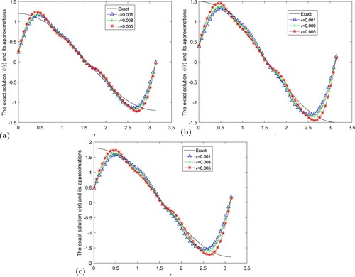
Figure 1. The exact solution and regular solution of Landweber regularization method by using the a posteriori parameter choice rule for Example 5.1. (a) $\alpha =1.2$, (b) $\alpha =1.5$, (c) $\alpha =1.8$.

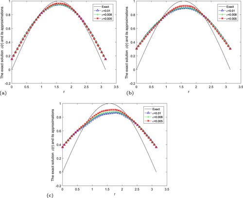
Figure 2. The exact solution and regular solution of fractional Landweber regularization method by using the a posteriori parameter choice rule for Example 5.1. (a) $\alpha =1.2$, (b) $\alpha =1.5$, (c) $\alpha =1.8$.

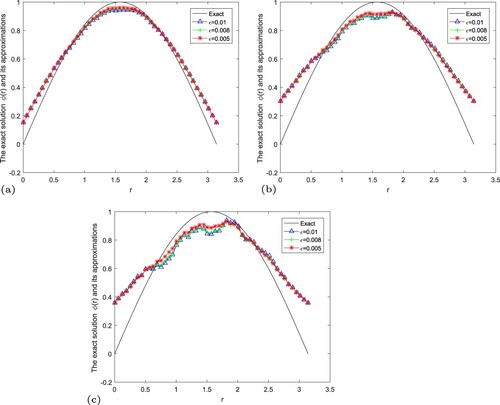
Figure 3. The exact solution and regular solution of modified iterative regularization method by using the a posteriori parameter choice rule for Example 5.1. (a) $\alpha =1.2$, (b) $\alpha =1.5$, (c) $\alpha =1.8$.

Example 5.2

Take function $\phi \left(r\right)=\left\{\begin{array}{ll}2r,& 0<r<\frac{\pi }{2},\\ 2(\pi -r),& \frac{\pi }{2}\le r<\pi .\end{array}\right.$In Figures 4–6, we give numerical results of Example 5.2 under the a posteriori parameter choice rule for various noise levels $ϵ=0.01,0.008,0.005$ in the case of $\alpha =1.2,1.5,1.8$. It can be seen that the numerical error also decreases when the noise is reduced. And the smaller α, the better the approximate effect.

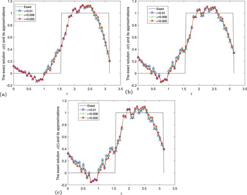
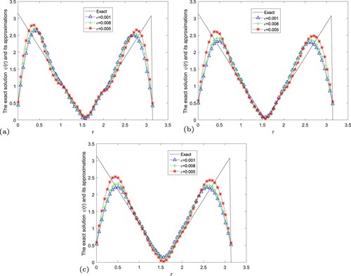
Figure 4. The exact solution and regular solution of Landweber regularization method by using the a posteriori parameter choice rule for Example 5.2. (a) $\alpha =1.2$, (b) $\alpha =1.5$, (c) $\alpha =1.8$.

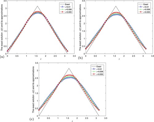
Figure 5. The exact solution and regular solution of fractional Landweber regularization method by using the a posteriori parameter choice rule for Example 5.2. (a) $\alpha =1.2$, (b) $\alpha =1.5$, (c) $\alpha =1.8$.

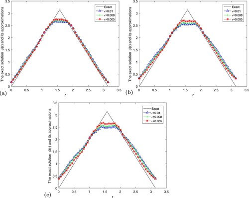
Figure 6. The exact solution and regular solution of modified iterative regularization method by using the a posteriori parameter choice rule for Example 5.2. (a) $\alpha =1.2$, (b) $\alpha =1.5$, (c) $\alpha =1.8$.

We fix $ϵ=0.01$. For Table 1, when $\alpha =1.2$, the iterative steps of Landweber regularization method, fractional Landweber regularization method and modified iterative method are 597, 75 and 137. When $\alpha =1.5$, the iterative steps of Landweber regularization method, fractional Landweber regularization method and modified iterative method are 272, 41 and 67. When $\alpha =1.8$, the iterative steps of Landweber regularization method, fractional Landweber regularization method and modified iterative method are 262, 42 and 67. We can deduce that $ϵ=0.01$ is fixed, the fractional Landweber regularization method has fewer iteration steps. For $ϵ=0.008$ and $ϵ=0.005$, the same result is obtained.

Table 1. The iteration steps of Example 5.1 for different regularization method.

ε		0.01	0.008	0.005
Landweber	$\alpha =1.2$	597	766	1362
	$\alpha =1.5$	272	386	687
	$\alpha =1.8$	262	378	679
Fractional Landweber	$\alpha =1.2$	75	93	138
	$\alpha =1.5$	41	52	85
	$\alpha =1.8$	42	52	83
Modified iterative	$\alpha =1.2$	137	170	261
	$\alpha =1.5$	67	91	155
	$\alpha =1.8$	67	89	153

We fix $\alpha =1.2$. When $ϵ=0.01$, the iterative steps of Landweber regularization method, fractional Landweber regularization method and modified iterative method are 597, 75 and 137. When $ϵ=0.008$, the iterative steps of Landweber regularization method, fractional Landweber regularization method and modified iterative method are 766, 93 and 170. When $ϵ=0.005$, the iterative steps of Landweber regularization method, fractional Landweber regularization method and modified iterative method are 1362, 138 and 261. We can deduce that $\alpha =1.2$ is fixed, the fractional

Landweber regularization method has fewer iteration steps. For $\alpha =1.5$ and $\alpha =1.8$, the same result is obtained.

In summary, the fractional Landweber regularization method has fewer iteration steps.

In Table 2, we use a computer with Intel(R) Core(TM) i5-6200U CPU @ 2.30 GHz 2.40 GHz and RAM of 4.00 GB to calculate the CPU time. The specific analysis is as follows: we fix $\alpha =1.2$. For Table 2, when $ϵ=0.01$, the CPU time of Landweber regularization method, fractional Landweber regularization method and modified iterative method are 11.9304 s, 1.7742 s and 2.8694 s. When $ϵ=0.008$, the CPU time of Landweber regularization method, fractional Landweber regularization method and modified iterative method are 15.4281 s, 1.5056 s and 3.4975 s. When $ϵ=0.005$, the CPU time of Landweber regularization method, fractional Landweber regularization method and modified iterative method are 27.4445 s, 2.4426 s and 5.4024 s. We can deduced that $\alpha =1.2$ is fixed, the fractional Landweber regularization method has fewer CPU time. For $\alpha =1.5$ and $\alpha =1.8$, the same result is obtained.

Table 2. The CPU time of Example 5.1 for different regularization method.

α		1.2	1.5	1.8
Landweber	$ϵ=0.01$	11.9304	5.8485	5.7179
	$ϵ=0.008$	15.4281	7.4576	7.5216
	$ϵ=0.005$	27.4445	13.4199	13.4263
Fractional Landweber	$ϵ=0.01$	1.7742	0.6786	0.7475
	$ϵ=0.008$	1.5056	1.4258	1.4617
	$ϵ=0.005$	2.4426	1.4684	1.5987
Modified iterative	$ϵ=0.01$	2.8694	1.6987	1.7893
	$ϵ=0.008$	3.4975	1.5797	1.4896
	$ϵ=0.005$	5.4024	3.4720	3.4510

We fix $ϵ=0.01$. When $\alpha =1.2$, the CPU time of Landweber regularization method, fractional Landweber regularization method and modified iterative method are 11.9304 s, 1.7742 s and 2.8694 s. When $\alpha =1.5$, the CPU time of Landweber regularization method, fractional Landweber regularization method and modified iterative method are 5.8485 s, 0.6786 s and 1.6987 s. When $\alpha =1.8$, the CPU time of Landweber regularization method, fractional Landweber regularization method and modified iterative method are 5.7179 s, 0.7475 s and 1.7893 s. We can deduced that $ϵ=0.01$ is fixed, the fractional Landweber regularization method has fewer CPU time. For $ϵ=0.008$ and $ϵ=0.005$, the same result is obtained. In summary, the fractional Landweber regularization method has fewer CPU time.

By Table 3, we can deduce that the errors between exact solution and approximate solution are smaller for fixed α and the smaller measurement error. And we infer that the error between exact solution and approximation solution of fractional Landweber method is smaller than that obtained by Landweber regularization method and modified iterative method for fixed α and ε.

Table 3. Error behaviour of Example 5.1 for different α with $ϵ=0.01,0.005$.

α			1.1	1.3	1.5	1.7	1.9
Landweber	$ϵ=0.01$	Rela	0.7320	0.6001	0.5101	0.3923	0.2431
	$ϵ=0.01$	Abso	0.6078	0.4319	0.3121	0.1920	0.1311
	$ϵ=0.005$	Rela	0.6501	0.5017	0.3725	0.2519	0.0935
	$ϵ=0.005$	Abso	0.5910	0.4270	0.2110	0.1175	0.0734
Fractional Landweber	$ϵ=0.01$	Rela	0.4560	0.3817	0.3039	0.2377	0.2105
	$ϵ=0.01$	Abso	0.2113	0.1352	0.0987	0.0553	0.0098
	$ϵ=0.005$	Rela	0.2715	0.1219	0.0902	0.0835	0.0631
	$ϵ=0.005$	Abso	0.1091	0.0836	0.0430	0.0259	0.0047
Modified iterative	$ϵ=0.01$	Rela	0.5734	0.5180	0.3945	0.3030	0.2509
	$ϵ=0.01$	Abso	0.3978	0.2534	0.2575	0.1114	0.0273
	$ϵ=0.005$	Rela	0.3807	0.3741	0.2370	0.1415	0.0901
	$ϵ=0.005$	Abso	0.2933	0.1717	0.1682	0.0807	0.0109

From Table 4, we can obtain the error between exact solution and approximation solution of fractional Landweber method is smaller than that obtained by Landweber regularization method and modified iterative method for fixed α and ε.

Table 4. Error behaviour of Example 5.2 for different α with $ϵ=0.01,0.005$.

α			1.1	1.3	1.5	1.7	1.9
Landweber	$ϵ=0.01$	Rela	0.9845	0.7516	0.5322	0.3303	0.2730
	$ϵ=0.01$	Abso	0.7814	0.5831	0.4911	0.2510	0.1425
	$ϵ=0.005$	Rela	0.9013	0.6289	0.4516	0.2035	0.1013
	$ϵ=0.005$	Abso	0.6317	0.5521	0.3849	0.1228	0.0616
Fractional Landweber	$ϵ=0.01$	Rela	0.4532	0.3907	0.3015	0.2072	0.1723
	$ϵ=0.01$	Abso	0.3017	0.2125	0.1526	0.0821	0.0101
	$ϵ=0.005$	Rela	0.2853	0.2036	0.1489	0.0956	0.0745
	$ϵ=0.005$	Abso	0.1350	0.1049	0.0731	0.0232	0.0059
Modified iterative	$ϵ=0.01$	Rela	0.6711	0.5332	0.4136	0.2871	0.2020
	$ϵ=0.01$	Abso	0.3506	0.3029	0.2207	0.1019	0.0310
	$ϵ=0.005$	Rela	0.3421	0.2521	0.1987	0.1115	0.0109
	$ϵ=0.005$	Abso	0.1823	0.1352	0.0908	0.0673	0.0456

In Figures 1–3, we give numerical results of Example 5.1 under the a posteriori parameter choice rule for various noise levels $ϵ=0.01,0.008,0.005$ in the case of $\alpha =1.2,1.5,1.8$. It can be seen that the numerical error also decreases when the noise is reduced. And the smaller α, the better the approximate effect.

In Figures 4–6, we give numerical results of Example 5.2 under the a posteriori parameter choice rule for various noise levels $ϵ=0.01,0.008,0.005$ in the case of $\alpha =1.2,1.5,1.8$. It can be seen that the numerical error also decreases when the noise is reduced. And the smaller α, the better the approximate effect.

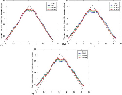
In Figures 7–9, we give numerical results of Example 5.3 under the a posteriori parameter choice rule for various noise levels $ϵ=0.01,0.008,0.005$ in the case of $\alpha =1.2,1.5,1.8$. It can be seen that the numerical error also decreases when the noise is reduced. And the smaller α, the better the approximate effect.

Figure 7. The exact solution and regular solution of Landweber regularization method by using the a posteriori parameter choice rule for Example 5.3. (a) $\alpha =1.2$, (b) $\alpha =1.5$, (c) $\alpha =1.8$.

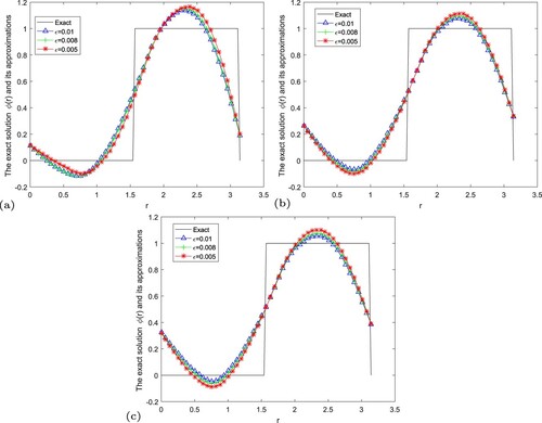
Figure 8. The exact solution and regular solution of fractional Landweber regularization method by using the a posteriori parameter choice rule for Example 5.3. (a) $\alpha =1.2$, (b) $\alpha =1.5$, (c) $\alpha =1.8$.

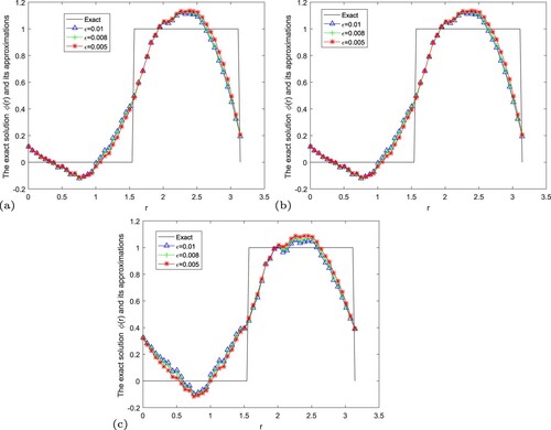
Figure 9. The exact solution and regular solution of modified iterative regularization method by using the a posteriori parameter choice rule for Example 5.3. (a) $\alpha =1.2$, (b) $\alpha =1.5$, (c) $\alpha =1.8$.

Example 5.3

Take function $\phi \left(r\right)=\left\{\begin{array}{ll}0,& 0<r\le \frac{\pi }{2},\\ 1,& \frac{\pi }{2}<r<\pi .\end{array}\right.$

In Figures 10–12, we give numerical results of Example 5.4 under the a posteriori parameter choice rule for various noise levels $ϵ=0.01,0.008,0.005$ in the case of $\alpha =1.2,1.5,1.8$. It can be seen that the numerical error also decreases when the noise is reduced. And the smaller α, the better the approximate effect.

Figure 10. The exact solution and regular solution of Landweber regularization method by using the a posteriori parameter choice rule for Example 5.4. (a) $\alpha =1.2$, (b) $\alpha =1.5$, (c) $\alpha =1.8$.

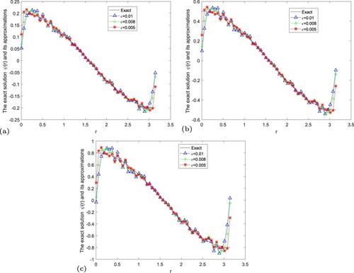
Figure 11. The exact solution and regular solution of fractional Landweber regularization method by using the a posteriori parameter choice rule for Example 5.4. (a) $\alpha =1.2$, (b) $\alpha =1.5$, (c) $\alpha =1.8$.

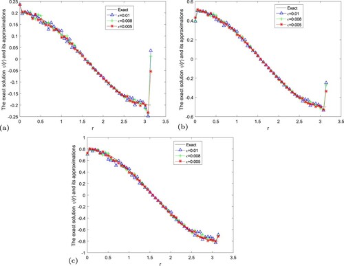
Figure 12. The exact solution and regular solution of modified iterative regularization method by using the a posteriori parameter choice rule for Example 5.4. (a) $\alpha =1.2$, (b) $\alpha =1.5$, (c) $\alpha =1.8$.

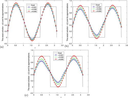
In Figures 13–15, we give numerical results of Example 5.5 under the a posteriori parameter choice rule for various noise levels $ϵ=0.01,0.008,0.005$ in the case of $\alpha =1.2,1.5,1.8$. It can be seen that the numerical error also decreases when the noise is reduced. And the smaller α, the better the approximate effect.

Figure 13. The exact solution and regular solution of Landweber regularization method by using the a posteriori parameter choice rule for Example 5.5. (a) $\alpha =1.2$, (b) $\alpha =1.5$, (c) $\alpha =1.8$.

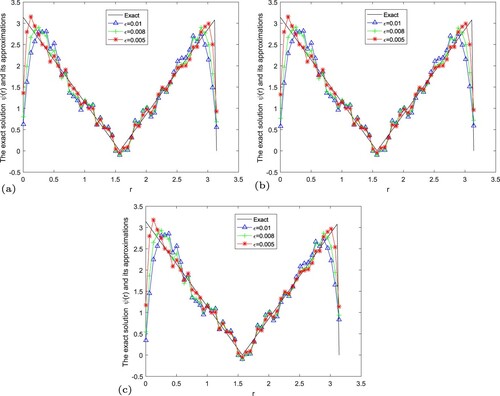
Figure 14. The exact solution and regular solution of fractional Landweber regularization method by using the a posteriori parameter choice rule for Example 5.5. (a) $\alpha =1.2$, (b) $\alpha =1.5$, (c) $\alpha =1.8$.

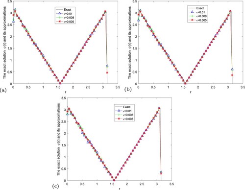
Figure 15. The exact solution and regular solution of modified iterative regularization method by using the a posteriori parameter choice rule for Example 5.5. (a) $\alpha =1.2$, (b) $\alpha =1.5$, (c) $\alpha =1.8$.

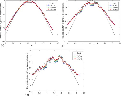
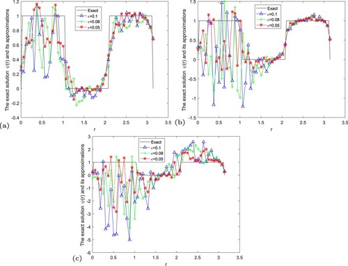
In Figures 16–18, we give numerical results of Example 5.6 under the a posteriori parameter choice rule for various noise levels $ϵ=0.01,0.008,0.005$ in the case of $\alpha =1.2,1.5,1.8$. It can be seen that the numerical error also decreases when the noise is reduced. And the smaller α, the better the approximate effect.

Figure 16. The exact solution and regularization solution of Landweber regularization method by using the a posteriori parameter choice rule for Example 5.6. (a) $\alpha =1.2$, (b) $\alpha =1.5$, (c) $\alpha =1.8$.

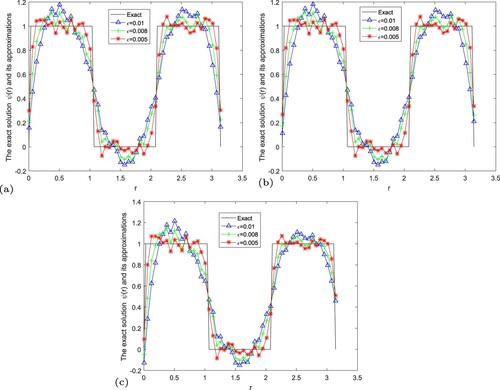
Figure 17. The exact solution and regularization solution of fractional Landweber regularization method by using the a posteriori parameter choice rule for Example 5.6. (a) $\alpha =1.2$, (b) $\alpha =1.5$, (c) $\alpha =1.8$.

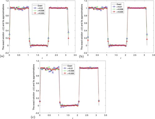
Figure 18. The exact solution and regularization solution of modified iterative method by using the a posteriori parameter choice rule for Example 5.6. (a) $\alpha =1.2$, (b) $\alpha =1.5$, (c) $\alpha =1.8$.

Example 5.4

Take function $\psi \left(r\right)=\alpha \cos \left(r\right)$.

Example 5.5

Take function $\psi \left(r\right)=\left\{\begin{array}{ll}-2r+\pi ,& 0<r\le \frac{\pi }{2},\\ 2r-\pi ,& \frac{\pi }{2}\le r<\pi .\end{array}\right.$

Example 5.6

Take function $\psi \left(r\right)=\left\{\begin{array}{ll}1,& 0<r\le \frac{\pi }{3},\\ 0,& \frac{\pi }{3}<r\le \frac{2\pi }{3},\\ 1,& \frac{2\pi }{3}<r<\pi .\end{array}\right.$From the above conclusion, we know that the fractional Landweber regularization method is the most efficient and accurate. Next, the error of the regular solution and the exact solution is given in Figure 19 under the rule of selecting the posterior regularization parameters when we choose $ϵ=0.01,0.05,0.08$, respectively. We can know that if the noise levels becomes lager, the error between the exact solution and the regular solution by using the a posteriori parameter choice rule will become lager.

Figure 19. The exact solution and regular solution of fractional Landweber regularization method by using the a posteriori parameter choice rule for Example 5.6. (a) $\alpha =1.2$, (b) $\alpha =1.5$, (c) $\alpha =1.8$.

We can deduce that when ε and α are larger, the error between the exact solution and the regular solution by using the a posteriori parameter choice rule is greater.

6. Conclusion

An inverse problem for the time-fractional diffusion-wave equation on spherically symmetric domain is considered. Based on the conditional stability, we propose Landweber regularization method, fractional Landweber regularization method and modified iterative method to deal with the problem and derive the a-priori and a posteriori convergence eatimate. In addition, numerical examples verify that the fractional Landweber iterative regularization method is more efficient and accurate. In the following research work, I will continue to study the inverse problems of some equations on special regions, such as cylindrical symmetric regions or spherically symmetric regions, which should be very interesting, and then use appropriate regularization methods to solve them.

Disclosure statement

No potential conflict of interest was reported by the author(s).

Additional information

Funding

The project is supported by the National Natural Science Foundation of China [No. 11961044], the Doctor Fund of Lan Zhou University of Technology.

Appendix

Proof

Proof of Lemma 2.3

We define two functions with ${\tau }_1^2:=a_1{E}_{\alpha ,1}^2(-{\lambda }_n{T}^{\alpha })$: $\phi \left({\tau }_1\right)=a_1[1-(1-{\tau }_1^2{)}^{m_1}{]}^{2\gamma }{\tau }_1^{-2},$and $\varphi \left({\tau }_1\right)=[1-(1-{\tau }_1^2{)}^{m_1}{]}^{2\gamma }{\tau }_1^{-2}.$Obviously $\phi \left({\tau }_1\right)=a_1\varphi \left({\tau }_1\right)$. These two functions are continuous when ${\tau }_1\in (0,1)$.

For $\frac{1}{2}<\gamma <1$ and ${\tau }_1\in (0,1)$, using Lemma 3.3 in [63], we have $\varphi \left({\tau }_1\right)\le m_1$. Therefore, $\underset{{\lambda }_n>0}{sup}[1-(1-a_1{E}_{\alpha ,1}^2(-{\lambda }_n{T}^{\alpha }){)}^{m_1}{]}^{\gamma }\frac{1}{E_{\alpha ,1}(-{\lambda }_n{T}^{\alpha })}\le \sqrt{a_1{m}_1}.$The proof of (9(9) $\begin{array}{rl}& \underset{{\lambda }_n>0}{sup}[1-(1-a_2{T}^2{E}_{\alpha ,2}^2(-{\lambda }_n{T}^{\alpha }){)}^{m_2}{]}^{\gamma }\frac{1}{T{E}_{\alpha ,2}(-{\lambda }_n{T}^{\alpha })}\le \sqrt{a_2{m}_2}.\end{array}$(9) ) is similar, so it is omitted.

Proof

Proof of Lemma 2.4

We introduce a new variable $x:=E_{\alpha ,1}^2(-{\lambda }_n{T}^{\alpha })<1/a_1$ and define a function $h\left(x\right)=(1-a_{1}x{)}^{m_1}{x}^{\frac{p}{4}}$. It is easy to verify that there exists a unique $x_0=\frac{z}{a_1(z+m_1)}$ with $z=\frac{p}{4}$ such that $h^{\prime }\left(x_0\right)=0$, we then have $\begin{array}{rl}h\left(x\right)& \le h\left(x_0\right)\le {\left(1-\frac{z}{z+m_1}\right)}^{m_1}{\left(\frac{z}{a_1\left(z+m_1\right)}\right)}^z<{\left(\frac{z}{a_1}\right)}^z{\left(\frac{1}{z+m_1}\right)}^z\\ & <{\left(\frac{z}{a_1}\right)}^z{\left(\frac{1}{m_1}\right)}^z:=c(a_1,p)m_1^{-\frac{p}{4}}.\end{array}$The proof of (11(11) $\begin{array}{rl}& \underset{{\lambda }_n>0}{sup}(1-a_2{T}^2{E}_{\alpha ,2}^2(-{\lambda }_n{T}^{\alpha }\left){)}^{m_2}{T}^{\frac{p}{2}}{E}_{\alpha ,2}^{\frac{p}{2}}\right(-{\lambda }_n{T}^{\alpha })\le c(a_2,p)m_2^{-\frac{p}{4}},\end{array}$(11) ) is similar, so it is omitted.

Proof

Proof of Lemma 2.7

From Lemma 2.6, we have ${\left(1-a_1{E}_{\alpha ,1}^2\left(-{\left(\frac{n\pi }{r_0}\right)}^2{T}^{\alpha }\right)\right)}^{m_3}(1+n^2{)}^{-\frac{p}{2}}\le {\left(1-a_1\frac{{\underset{\_}{C}}^2{r}_0^4}{n^4{\pi }^4}\right)}^{m_3}(n^2{)}^{-\frac{p}{2}}.$Define $x:=n^2$, $F\left(x\right):={\left(1-a_1\frac{{\underset{\_}{C}}^2{r}_0^4}{x^2{\pi }^4}\right)}^{m_3}{x}^{-\frac{p}{2}},$it is easy to find the unique point $x_0=(\frac{a_1{\underset{\_}{C}}^2{r}_0^4}{{\pi }^4}\cdot \frac{4m_3+p}{p}{)}^{\frac{1}{2}}$ such that $F^{\mathrm{\prime }}\left(x_0\right)=0$. Therefore $\begin{array}{rl}F\left(x\right)& \le F\left(x_0\right)\le {\left[1-\frac{a_1{\underset{\_}{C}}^2{r}_0^4}{{\pi }^4}\cdot \frac{p{\pi }^4}{a_1{\underset{\_}{C}}^2{r}_0^4(4m_3+p)}\right]}^{m_3}{\left(\frac{p{\pi }^4}{a_1{\underset{\_}{C}}^2{r}_0^4(4m_3+p)}\right)}^{\frac{p}{4}}\\ & \le {\left(\frac{a_1{\underset{\_}{C}}^2{r}_0^4}{p{\pi }^4}\right)}^{\frac{p}{4}}(m_3+1{)}^{-\frac{p}{4}}.\end{array}$The proof of (15(15) $\begin{array}{rl}& {\left(1-a_2{T}^2{E}_{\alpha ,2}^2\left(-{\left(\frac{n\pi }{r_0}\right)}^2{T}^{\alpha }\right)\right)}^{m_4}(1+n^2{)}^{-\frac{p}{2}}\le C_4(m_4+1{)}^{-\frac{p}{4}},\end{array}$(15) ) is similar, so it is omitted.

Proof

Proof of Lemma 2.8

For the first inequality, we have the following results. From Lemma 2.6, we have ${\left(1-a_1{E}_{\alpha ,1}^{\gamma +1}\left(-{\left(\frac{n\pi }{r_0}\right)}^2{T}^{\alpha }\right)\right)}^{m_5}(1+n^2{)}^{-\frac{p}{2}}\le {\left(1-a_1{\left(\frac{\underset{\_}{C}{r}_0^2}{n^2{\pi }^2}\right)}^{\gamma +1}\right)}^{m_5}(n^2{)}^{-\frac{p}{2}}.$Define $x:=n^2$, $F\left(x\right):={\left(1-a_1{\left(\frac{\underset{\_}{C}{r}_0^2}{x{\pi }^2}\right)}^{\gamma +1}\right)}^{m_5}{x}^{-\frac{p}{2}},$it is easy to find the unique point $x_0=\frac{\underset{\_}{C}{r}_0^2}{{\pi }^2}(\frac{2a_1{m}_5(\gamma +1)}{p}+a_1{)}^{\frac{1}{\gamma +1}}$ such that $F^{\mathrm{\prime }}\left(x_0\right)=0$. Therefore $\begin{array}{rl}F\left(x\right)& \le F\left(x_0\right)={\left(\frac{2a_1{m}_5(\gamma +1)}{p}{\left(\frac{\underset{\_}{C}{r}_0^2}{{\pi }^2}\right)}^{\gamma +1}+a_1{\left(\frac{\underset{\_}{C}{r}_0^2}{{\pi }^2}\right)}^{\gamma +1}\right)}^{-\frac{p}{2(\gamma +1)}}\\ & ={\left(\frac{\underset{\_}{C}{r}_0^2}{{\pi }^2}\right)}^{-\frac{p}{2}}{\left(\frac{2a_1{m}_5(\gamma +1)}{p}+a_1\right)}^{-\frac{p}{2(\gamma +1)}}\\ & \le {\left(\frac{\underset{\_}{C}{r}_0^2}{{\pi }^2}\right)}^{-\frac{p}{2}}{\left(\frac{2a_1(\gamma +1)}{p}\right)}^{-\frac{p}{2(\gamma +1)}}{m}_5^{-\frac{p}{2(\gamma +1)}}.\end{array}$For the second inequality, we have the following inequality. From Lemma 2.6, we have ${\left(1-a_2{T}^{\gamma +1}{E}_{\alpha ,2}^{\gamma +1}\left(-{\left(\frac{n\pi }{r_0}\right)}^2{T}^{\alpha }\right)\right)}^{m_6}(1+n^2{)}^{-\frac{p}{2}}\le {\left(1-a_2{\left(\frac{\underset{\_}{C}T{r}_0^2}{n^2{\pi }^2}\right)}^{\gamma +1}\right)}^{m_6}(n^2{)}^{-\frac{p}{2}}.$Define $y:=n^2$, $G\left(y\right):={\left(1-a_2{\left(\frac{\underset{\_}{C}T{r}_0^2}{y{\pi }^2}\right)}^{\gamma +1}\right)}^{m_6}{y}^{-\frac{p}{2}},$it is easy to find the unique point $y_0=\frac{\underset{\_}{C}T{r}_0^2}{{\pi }^2}(\frac{2a_2{m}_6(\gamma +1)}{p}+a_2{)}^{\frac{1}{\gamma +1}}$ such that $G^{\mathrm{\prime }}\left(y_0\right)=0$. Therefore $\begin{array}{rl}G\left(y\right)& \le G\left(y_0\right)={\left(\frac{2a_2{m}_6(\gamma +1)}{p}{\left(\frac{\underset{\_}{C}{r}_0^2}{{\pi }^2}\right)}^{\gamma +1}+a_2{\left(\frac{\underset{\_}{C}{r}_0^2}{{\pi }^2}\right)}^{\gamma +1}\right)}^{-\frac{p}{2(\gamma +1)}}\\ & ={\left(\frac{\underset{\_}{C}{r}_0^2}{{\pi }^2}\right)}^{-\frac{p}{2}}{\left(\frac{2a_2{m}_6(\gamma +1)}{p}+a_2\right)}^{-\frac{p}{2(\gamma +1)}}\\ & \le {\left(\frac{\underset{\_}{C}{r}_0^2}{{\pi }^2}\right)}^{-\frac{p}{2}}{\left(\frac{2a_2(\gamma +1)}{p}\right)}^{-\frac{p}{2(\gamma +1)}}{m}_6^{-\frac{p}{2(\gamma +1)}}.\text{■}\end{array}$

Proof

Proof of Lemma 2.9

Let $f\left({\sigma }_{1n}\right):=(1-(1-a_1{\sigma }_{1n}^{\gamma +1}{)}^{m_5})/{\sigma }_{1n}$ and ${\sigma }_{1n}:=E_{\alpha ,1}(-(\frac{n\pi }{r_0}{)}^2{T}^{\alpha })$, ${\text{β}}_1:=a_1{\sigma }_{1n}^{\gamma +1}$, then ${\sigma }_{1n}=(\frac{{\text{β}}_1}{a_1}{)}^{\frac{1}{\gamma +1}}$ and $f\left({\text{β}}_1\right)=(1-(1-{\text{β}}_1{)}^{m_5}\left)\right({\text{β}}_1/a_1{)}^{-\frac{1}{\gamma +1}}$.

Since $0<a_1{E}_{\alpha ,1}^{\gamma +1}(-(\frac{n\pi }{r_0}{)}^2{T}^{\alpha })<1$, we have $0<{\text{β}}_1<1$. Hence from $0<\frac{1}{\gamma +1}<1$, $1-(1-{\text{β}}_1{)}^{m_5}<1$ and we have the following inequality holds, (A1) $\begin{array}{rl}f\left({\text{β}}_1\right)& =(1-(1-{\text{β}}_1{)}^{m_5}\left)\right({\text{β}}_1/a_1{)}^{-\frac{1}{\gamma +1}}\\ & \le (1-(1-{\text{β}}_1{)}^{m_5}{)}^{\frac{1}{\gamma +1}}({\text{β}}_1/a_1{)}^{-\frac{1}{\gamma +1}}\\ & ={\left(\frac{1-(1-{\text{β}}_1{)}^{m_5}}{{\text{β}}_1}\right)}^{\frac{1}{\gamma +1}}{a}_1^{\frac{1}{\gamma +1}}.\end{array}$(A1) Due to for $n\ge 0$ and $x\ge -1$, we have (A2) $(1+x{)}^n\ge 1+nx.$(A2) Combining (A1(A1) $\begin{array}{rl}f\left({\text{β}}_1\right)& =(1-(1-{\text{β}}_1{)}^{m_5}\left)\right({\text{β}}_1/a_1{)}^{-\frac{1}{\gamma +1}}\\ & \le (1-(1-{\text{β}}_1{)}^{m_5}{)}^{\frac{1}{\gamma +1}}({\text{β}}_1/a_1{)}^{-\frac{1}{\gamma +1}}\\ & ={\left(\frac{1-(1-{\text{β}}_1{)}^{m_5}}{{\text{β}}_1}\right)}^{\frac{1}{\gamma +1}}{a}_1^{\frac{1}{\gamma +1}}.\end{array}$(A1) ) and (A2(A2) $(1+x{)}^n\ge 1+nx.$(A2) ), we have $f\left({\text{β}}_1\right)\le (a_1{m}_5{)}^{\frac{1}{\gamma +1}}.$The proof of (19(19) $\begin{array}{rl}& \frac{1-{\left(1-a_2{T}^{\gamma +1}{E}_{\alpha ,2}^{\gamma +1}\left(-{\left({\displaystyle \frac{n\pi }{r_0}}\right)}^2{T}^{\alpha }\right)\right)}^{m_6}}{T{E}_{\alpha ,2}\left(-{\left({\displaystyle \frac{n\pi }{r_0}}\right)}^2{T}^{\alpha }\right)}\le (a_2{m}_6{)}^{\frac{1}{\gamma +1}}.\end{array}$(19) ) is similar, so it is omitted.

Proof

Proof of Lemma 2.10

If $x_0$ satisfies $F^{\prime }\left(x_0\right)=0$, we obtain $x_0={\left(\frac{a_1\underset{\_}{C}{r}_0^4}{{\pi }^4}\cdot \frac{4m_1+p-2}{p+2}\right)}^{\frac{1}{2}},$therefore, we have $F\left(x\right)\le F\left(x_0\right)\le \frac{\overline{C}{r}_0^2}{{\pi }^2}{\left(\frac{a_1\underset{\_}{C}{r}_0^4}{(p+2){\pi }^4}\right)}^{-\frac{p+2}{4}}(m_1+1{)}^{-\frac{p+2}{4}}.$The proof of (21(21) $\begin{array}{rl}G\left(x\right)& =\frac{T\overline{C}{r}_0^2}{{\pi }^2}{\left(1-\frac{a_2{T}^2{\underset{\_}{C}}^2{r}_0^4}{x^2{\pi }^4}\right)}^{m_2-1}(x{)}^{-\frac{p}{2}-1}\le C_8(m_2+1{)}^{-\frac{p+2}{4}},\end{array}$(21) ) is similar, so it is omitted.

Proof

Proof of Lemma 2.11

If $x_0$ satisfies $F^{\prime }\left(x_0\right)=0$, we obtain $x_0=\frac{\underset{\_}{C}{r}_0^2}{{\pi }^2}{\left(\frac{a_1}{p+2}\right)}^{\frac{1}{\gamma +1}}\left(\right(2m_5-2\left)\right(\gamma +1)+p+2{)}^{\frac{1}{\gamma +1}},$therefore, we have $F\left(x\right)\le F\left(x_0\right)\le \frac{\overline{C}{r}_0^2}{{\pi }^2}{\left(\frac{\underset{\_}{C}{r}_0^2}{{\pi }^2}\right)}^{-\frac{p}{2}-1}{\left(\frac{a_1}{p+2}\right)}^{-\frac{p+2}{2(\gamma +1)}}(m_5+1{)}^{-\frac{p+2}{2(\gamma +1)}}.$The proof of (23(23) $\begin{array}{rl}G\left(x\right)& =\frac{T\overline{C}{r}_0^2}{{\pi }^2}{\left(1-a_2{T}^{\gamma +1}{\left(\frac{\underset{\_}{C}{r}_0^2}{x{\pi }^2}\right)}^{\gamma +1}\right)}^{m_6-1}(x{)}^{-\frac{p}{2}-1}\le C_{10}(m_6+1{)}^{-\frac{p+2}{2(\gamma +1)}},\end{array}$(23) ) is similar, so it is omitted.

References

- Hall MG, Barrick TR. From diffusion-weighted MRI to anomalous diffusion imaging. Magnet Reson Med. 2008;59(3):447–455.
- Yuste SB, Acedo L, Lindenberg K. Reaction front in an A+B→C reaction-subdiffusion process. Phys Rev E. 2004;69(3):036126.
- Scalas E, Gorenflo R, Mainardi F. Fractional calculus and continuous-time finance. Phys A. 2000;284(1):376–384.
- Kohlmann M, Tang T. Fractional calculus and continuous-time finance III: the diffusion limit. In: Mathematical finance; 2001. p. 171–180, Birkhauser Verlag, Basel-Boton-Berlin.
- Meerschaert MM, Scalas E. Coupled continuous time random walks in finance. Phys A. 2006;370(1):114–118.
- Mainardi F, Raberto M, Gorenflo R, et al. Fractional calculus and continuous-time finance II: the waiting-time distribution. Phys A. 2000;287(3-4):468–481.
- Li ZX. An iterative ensemble Kalman method for an inverse scattering problem in acoustics. Mod Phys Lett B. 2020;34(28):12.
- Luchko Y. Initial-boundary-value problems for the generalized multi-term time-fractional diffusion equation. J Math Anal Appl. 2011;374(2):538–548.
- Luchko Y. Some uniqueness and existence results for the initial-boundary value problems for the generalized time-fractional diffusion equation. Comput Math Appl. 2010;59(5):1766–1772.
- Luchko Y. Initial-boundary-value problems for the one-dimensional time-fractional diffusion equation. Fract Calc Appl Anal. 2012;15(1):141–160.
- Luchko Y. Maximum principle for the generalized time-fractional diffusion equation. J Math Anal Appl. 2009;351(1):218–223.
- Li ZY, Luchko Y, Yamamoto M. Asymptotic estimates of solutions to initial-boundary-value problems for distributed order time-fractional diffusion equations. Fract Calc Appl Anal. 2014;17(4):1114–1136.
- Hossein J, Afshin B, Seddigheh B. A novel approach for solving an inverse reaction-diffusion-convection problem. J Optim Theory Appl. 2019;183(2):688–704.
- Afshin B, Seddigheh B. Reconstructing unknown nonlinear boundary conditions in a time-fractional inverse reaction-diffusion-convection problem. Numer Meth Part D E. 2019;35(3):976–992.
- Luchko Y. Boundary value problems for the generalized time-fractional diffusion equation of distributed order. Fract Calc Appl Anal. 2009;12(4):409–422.
- Bai ZB, Qiu TT. Existence of positive solution for singular fractional differential equation. Appl Math Comput. 2008;215(7):2761–2767.
- Kemppainen J. Existence and uniqueness of the solution for a time-fractional diffusion equation. Fract Calc Appl Anal. 2011;14(3):411–417.
- Wang JG, Wei T. Quasi-reversibility method to identify a space-dependent source for the time-fractional diffusion equation. Appl Math Model. 2015;39(20):6139–6149.
- Zhang ZQ, Wei T. Identifying an unknown source in time-fractional diffusion equation by a truncation method. Appl Math Comput. 2013;219(11):5972–5983.
- Wang JG, Zhou YB, Wei T. Two regularization methods to identify a space-dependent source for the time-fractional diffusion equation. Appl Numer Math. 2013;68(68):39–57.
- Yang F, Fu CL, Li XX. A quasi-boundary value regularization method for determining the heat source. Math Method Appl Sci. 2015;37(18):3026–3035.
- Yang F, Fu CL. The quasi-reversibility regularization method for identifying the unknown source for time fractional diffusion equation. Appl Math Model. 2015;39(5-6):1500–1512.
- Yang F, Fu CL, Li XX. Identifying an unknown source in space-fractional diffusion equation. Acta Math Sci. 2014;34(4):1012–1024.
- Yang F, Fu CL, Li XX. The inverse source problem for time fractional diffusion equation: stability analysis and regularization. Inverse Probl Sci Eng. 2015;23(6):969–996.
- Yang F, Ren YP, Li XX, et al. Landweber iterative method for identifying a space-dependent source for the time-fractional diffusion equation. Bound Value Probl. 2017;2017(1):163.
- Yang F, Liu X, Li XX. Landweber iterative regularization method for identifying the unknown source of the time-fractional diffusion equation. Adv Differ Equ. 2017;2017(1):388.
- Zheng GH, Wei T. Two regularization methods for solving a Riesz–Feller space-fractional backward diffusion problem. Inverse Probl. 2010;26:115017(22pp).
- Cheng H, Fu CL. An iteration regularization for a time-fractional inverse diffusion problem. Appl Math Model. 2012;36(11):5642–5649.
- Liu JJ, Yamamoto M. A backward problem for the time-fractional diffusion equation. Appl Anal. 2010;89(11):1769–1788.
- Yang F, Ren YP, Li XX. The quasi-reversibility method for a final value problem of the time-fractional diffusion equation with inhomogeneous source. Math Method Appl Sci. 2018;41(5):1774–1795.
- Wang LY, Liu JJ. Data regularization for a backward time-fractional diffusion problem. Comput Math Appl. 2012;64(11):3613–3626.
- Wang JG, Zhou YB, Wei T. A posteriori regularization parameter choice rule for the quasi-boundary value method for the backward time-fractional diffusion problem. Appl Math Lett. 2013;26(7):741–747.
- Tuan NH, Long LD, Nguyen VT, et al. On a final value problem for the time-fractional diffusion equation with inhomogeneous source. Inverse Probl Sci Eng. 2017;25(9):1367–1395.
- Taghavi A, Babaei A, Mohammadpour A. A stable numerical scheme for a time fractional inverse parabolic equation. Inverse Probl Sci Eng. 2017;25(10):1474–1491.
- Yang F, Zhang Y, Li XX. The quasi-boundary value regularization method for identifying the initial value with discrete random noise. Bound Value Probl. 2018;2018(1):108.
- Yang F, Zhang Y, Liu X, et al. The Quasi-boundary value method for identifying the initial value of the space-time an fractional diffusion equation. Acta Math Sci. 2020;40B(3):641–658.
- Yang F, Pu Q, Li XX. The fractional Tikhonov regularization methods for identifying the initial value problem for a time-fractional diffusion equation. J Comput Appl Math. 2020;380:112998.
- Ozbilge E, Demir A. Inverse problem for a time-fractional parabolic equation. J Inequal Appl. 2015;2015(1):81.
- Babaei A, Banihashemi S. A stable numerical approach to solve a time-fractional inverse heat conduction problem. Iran J Sci Technol A. 2018;42(4):2225–2236.
- Ruan ZS, Yang J, Lu XL. Tikhonov regularisation method for simultaneous inversion of the source term and initial data in a time-fractional diffusion equation. E Asian J Appl Math. 2015;5(3):273–300.
- Yang F, Zhang P, Li XX, et al. Tikhonov regularization method for identifying the space-dependent source for time-fractional diffusion equation on a columnar symmetric domain. Adv Differ Equ. 2020;2020:128.
- Li GS, Zhang DL, Jia XZ, et al. Simultaneous inversion for the space-dependent diffusion coefficient and the fractional order in the time-fractional diffusion equation. Inverse Probl. 2013;29:065014.
- Yang F, Ren YP, Li XX. Landweber iteration regularization method for identifying unknown source on a columnar symmetric domain. Inverse Probl Sci Eng. 2018;26(8):1109–1129.
- Cheng W, Zhao LL, Fu CL. Source term identification for an axisymmetric inverse heat conduction problem. Comput Math Appl. 2010;59(1):142–148.
- Cheng W, Ma YJ, Fu CL. Identifying an unknown source term in radial heat conduction. Inverse Probl Sci Eng. 2012;20(3):335–349.
- Yang F, Sun YR, Li XX. The quasi-boundary value method for identifying the initial value of heat equation on a columnar symmetric domain. Numer Algor. 2019;82(2):623–639.
- Cheng W, Fu CL. A modified Tikhonov regularization method for an axisymmetric backward heat equation. Acta Math Sin. 2010;26(11):2157–2164.
- Djerrar I, Alem L, Chorfi L. Regularization method for the radially symmetric inverse heat conduction problem. Bound Value Probl. 2017;2017(1):159.
- Xiong XT, Ma XJ. A backward identifying problem for an axis-symmetric fractional diffusion equation. Math Model Anal. 2017;22(3):311–320.
- Yang F, Wang N, Li XX. A quasi-boundary regularization method for identifying the initial value of time-fractional diffusion equation on spherically symmetric domain. J Inverse Ill-Posed Probl. 2019;27(5):609–621.
- Šišková K, Slodička M. Identification of a source in a fractional wave equation from a boundary measyrement. J Comput Appl Math. 2019;349:172–186.
- Liao KF, Li YS, Wei T. The identification of the time-dependent source term in time-fractional diffusion-wave equations. E Asian J Appl Math. 2019;9(2):330–354.
- Šišková K, Slodička M. Recognition of a time-dependent source in a time-fractional wave equation. Appl Numer Math. 2017;121:1–17.
- Gong XH, Wei T. Reconstruction of a time-dependent source term in a time-fractional diffusion-wave equation. Inverse Probl Sci Eng. 2019;27(11):1577–1594.
- Yang F, Pu Q, Li XX, et al. The truncation regularization method for identifying the initial value on non-homogeneous time-fractional diffusion-wave equations. Mathematics. 2019;7(11):1007.
- Yang F, Zhang Y, Li XX. Landweber iterative method for identifying the initial value problem of the time-space fractional diffusion-wave equation. Numer Algor. 2020;83(4):1509–1530.
- Wei T, Zhang Y. The backward problem for a time-fractional diffusion-wave equation in a bounded domain. Comput Math Appl. 2018;75(10):3632–3648.
- Xian J, Wei T. Determination of the initial data in a time-fractional diffusion-wave problem by a final time data. Comput Math Appl. 2019;78(8):2525–2540.
- Yang F, Wang N, Li XX. Landweber iterative method for an inverse source problem of time-fractional diffusion-wave equation on spherically symmetric domain. J Appl Anal Comput. 2020;10(2):514–529.
- Sakamoto K, Yamamoto M. Initial value/boundary value problems for fractional diffusion-wave equations and applications to some inverse problems. J Math Anal Appl. 2011;382(1):426–447.
- Murio DA. Implicit finite difference approximation for time fractional diffusion equations. Comput Math Appl. 2008;56(4):1138–1145.
- Zhuang P, Liu F. Implicit difference approximation for the time fractional diffusion equation. J Appl Math Comput. 2006;22(3):87–99.
- Klann E, Ramlau R. Regularization by fractional filter methods and data smoothing. Inverse Probl. 2008;24(2):025018.
- Han YZ, Xiong XT, Xue XM. A fractional Landweber method for solving backward time-fractional diffusion problem. Comput Math Appl. 2019;78(1):81–91.
- Xiong XT, Xue XM, Qian Z. A modified iterative regularization method for ill-posed problems. Appl Numer Math. 2017;122:108–128.
- Abbaszadeh M, Dehghan M. Numerical and analytical investigations for neutral delay fractional damped diffusion-wave equation based on the stabilized interpolating element free Galerkin(IEFG) method. Appl Numer Math. 2019;145:488–506.
- Dehghan M, Abbaszadeh M. A finite difference/finite element technique with error estimate for space fractional tempered diffusion-wave equation. Comput Math Appl. 2018;75(8):2903–2914.
- Dehghan M, Abbaszadeh M. A Legendre spectral element method(ESM) based on the modified bases for solving neutral delay distributed-order fractional damped diffusion-wave equation. Math Method Appl Sci. 2018;41(9):3476–3494.
- Abbaszadeh M, Dehghan M. An improved meshless method for solving two-dimensional distributed order time-fractional diffusion-wave equation with error estimate. Numer Algor. 2016;75(1):173–211.
- Irfan T. Fundamentals of MATLAB language; 2019.
- Irfan T. Introduction to MATLAB; 2019.