Inverse shape design method based on pressure and shear stress for separated flow via Elastic Surface Algorithm

Abstract

Elastic Surface Algorithm (ESA), which was proposed for the inverse design in external flows, substitutes the airfoil wall by an elastic curved beam that deforms due to a difference between the target and current pressure distributions. The original ESA, such as all inverse design methods, which use only pressure as the target parameter, cannot converge in separated flows because of an almost constant pressure inside the separated region. This study developed the ESA for the inverse design in external separated flows by considering a linear combination of normalized pressure and shear stress distribution as the target flow parameter. Removing the geometrical filtrations, the automatic determination of the beam elasticity modulus, and the definition of dynamic spines instead of the vertical spines were the other essential modifications to upgrade the ESA for separated flows. The method was verified for blunt-leading-edged airfoils in subsonic turbulent flow under different angles of attack, and different initially-guessed geometries. The method reduced the separation by modifying the wall shear stress along the separation region.

KEYWORDS:

• Hybrid inverse design
• Elastic Surface Algorithm
• shear stress
• pressure
• external flow
• separation
• subsonic
• blunt-leading-edged airfoil

2010 Mathematics Subject Classifications:

• 76M21
• 76D55
• 76D05
• 76D10

Nomenclature

A0	=	cross section area of the beam
A1	=	a function of shape factor
A3	=	a function of shape factor
AOA	=	Angle of Attack
b	=	width of the beam (normal to the plane)
BSA	=	Ball-Spine Algorithm
CPD	=	Current Pressure Distribution
$C_d$	=	drag coefficient
$C_{d\mathbf{\text{F}}}$	=	friction drag coefficient
$C_{d\mathbf{\text{P}}}$	=	pressure drag coefficient
$C_f$	=	friction coefficient
$C_l$	=	lift coefficient
$C_l/C_d$	=	lift-to-drag ratio
d	=	differential of a scalar variable
E	=	elasticity modulus
E0	=	initial value of elasticity modulus
e	=	axial strain
ESA	=	Elastic Surface Algorithm
ESM	=	Elastic Surface Method
f	=	external force vector of the curved beam
FEM	=	Finite Element Method
FEM-RMS	=	the residual of nodal displacements
FSA	=	Flexible String Algorithm
G	=	shear modulus
H	=	shape factor in external viscous fluid flow
I0	=	moment of inertia of the beam
K	=	total stiffness matrix of the curved beam
Ke	=	stiffness matrix of the element
L0	=	beam length in the reference configuration
LE	=	Leading Edge
M	=	bending moment in the current configuration
M0	=	bending moment in the reference configuration
N	=	axial force in the current configuration
n	=	number of curved beam nodes
N0	=	axial force in the reference configuration
P	=	static pressure (pa)
p	=	internal force vector of the beam
P*	=	normalized static pressure
$P_0$	=	total pressure (pa)
Q	=	dimensionless parameter for determination of elasticity modulus
$R{e}_{\theta }$	=	local Re based on momentum thickness
S	=	local nodal coordinate on the airfoil wall
S*	=	dimensionless local nodal coordinate
SST	=	Shear Stress Transport
t	=	thickness of the beam
TE	=	Trailing Edge
TPD	=	Target Pressure Distribution
U	=	strain energy
Ue	=	flow velocity on the boundary layer edge
u	=	x-component of the flow velocity
u	=	nodal displacement vector of the element
${\mathbf{\text{u}}}_B$	=	nodal displacement vector of the curved beam
$u_X$	=	node displacement in X direction
$u_Y$	=	node displacement in Y direction
V	=	shear force in the current configuration
v	=	y-component of the flow velocity
V0	=	shear force in the reference configuration
α	=	coefficient of normalized pressure difference
β	=	normalized shear stress difference coefficient
Δ	=	difference
ΔH	=	hybrid flow parameter
δ	=	differential of a vector
δ(x)	=	boundary layer thickness over a flat plate
θ	=	momentum thickness
θ	=	cross section rotation
κ	=	curvature of the beam
μw	=	dynamic viscosity near the airfoil wall
ν	=	kinematic viscosity
ρ	=	density
τ	=	shear stress (pa)
τ*	=	normalized shear stress
τw	=	flow shear stress on the airfoil wall
φ	=	degree of freedom of each beam node
$\mathrm{\partial }$	=	partial differential of a variable

Subscripts

current	=	related to the current shape
i	=	related to the number of beam node
iteration	=	related to the iteration shape
target	=	related to the target shape

Superscripts

k	=	related to the current increment
k + 1	=	related to the next increment
T	=	related to the transposed of a vector
n	=	related to current displacement
n + 1	=	related to updated displacement

1. Introduction

Considerable efforts have been made to optimize the systems that include heat transfer or fluid flow in external and internal flows. The limitations and computational costs are the major challenges when using design methods. Direct methods, inverse design methods, and different optimization algorithms have been used for optimal shape design. The direct methods is based on geometry corrections using feedback from a flow analysis code, and relies heavily on the previous designer’s experience, which make them time-consuming and inefficient because of the trial-and-error process [1].

Many studies have recently used direct numerical optimization for the aerodynamic shape design. Various optimization algorithms such as adjoint method, evolutional algorithm or machine learning are coupled with a flow solver to reach the best cost function. The optimization methods are often time-consuming or mathematically complicated with a high computational cost. However, the freedom in selecting the multi-objective cost functions and applying the constraints are the benefits of the optimization methods.

Inverse design methods despite the direct methods calculate the geometry corresponding to a given flow variable distribution on the boundary (e.g. wall target pressure distribution). By improving the aforementioned flow parameter distributions, the geometry profile can be inversely designed to increase the aerodynamic load, decrease the drag force, or decrease the flow losses. Inverse design methods only calculate the unknown boundaries corresponding to the distribution of the target flow parameter along the boundaries, and they cannot obtain the optimal geometry. From the viewpoint of engineering application, the inverse problem technique is desirable because it requires a much smaller number of flow simulations than the numerical optimization does [2]. In fact, inverse design methods make a direct relationship between geometry corrections and target flow parameter, which cause the faster convergence rate.

Inverse design methods can be divided into two types: (a) coupled (non-iterative) and (b) decoupled (iterative) methods. The coupled methods use a formulation, in which the surface coordinates appear implicitly as dependent variables. Indirect transpiration techniques and stream-function-as-coordinate approaches are categorized as coupled methods [3,4].

The coupled or non-iterative methods provide a new form of governing equations, in which the geometry coordinates and the flow variables are integrated. Therefore, the desired geometry and flow variables are obtained directly. The main problem with coupled methods is the complexity of these new governing equations in viscous flow and complex geometries [5,6]. Stanitz [7] converted the physical space (x, y) into computational space (φ, ψ) to regenerate the inverse design equations from the Laplace equation in two-dimensional potential flows. In Stanitz’s method, the target velocity distribution along the boundaries should be given. When a coupled equation and its appropriate boundary conditions are solved, the x and y coordinates of the flow lines and equipotential lines, and the flow angles along the streamlines are obtained, which determines the boundary of the body [7]. Many researchers have used Stanitz’s method to solve boundary-shape design problems in internal and external flows [8]. Approximately thirty years after Stanitz solved the inverse design problems in two-dimensional potential flows, he presented an extended three-dimensional version of his method [9,10]. Zannetti [11] managed the inverse design form of the Euler equations in two-dimensional and axisymmetric flow by converting the physical space into computational space.

Ashrafizadeh et al. [12,13] presented a new element-based finite-volume discretization approach to solve incompressible flow problems on co-located grids. The proposed method, called the Method of Proper Closure Equations (MPCE), employed a proper set of physical relevant equations to constrain the velocity and pressure at the integration points.

A series of sequential problems can be solved using an iterative inverse design approach, and the geometry is modified at each shape modification step. The flow equations and the geometry modification equations are solved separately in these methods. The main advantages of the iterative inverse design methods is that the flow analysis codes such as commercial or open-source flow analysis software, which are developed in different regimes and complicated geometries, can easily be used to compute the required flow parameters on the target boundaries.

Some iterative inverse design methods are based on optimization algorithms to correct the geometry, and others use residual correction algorithms, which are mainly based on physical approaches [14]. The optimization-based inverse design methods, such as genetic algorithms and neural networks, are usually time-consuming or mathematically complicated with a high computational cost. These methods aim to reach a minimum difference between the current and target pressure distribution [15]. The residual correction methods use physical algorithms instead of mathematical algorithms to correct the geometry at each shape modification step. As a result, these methods have a higher convergence rate and a higher efficiency than optimization-based inverse design methods [16].

There are several inverse design methods [17–19] which are capable of determining the proper aerodynamic shape to satisfy a target pressure distribution on its surface. Most of these methods require the development of new complex mathematical formulations and the accompanying new solvers, which are time-consuming and not proper for industrial applications. Therefore, the iterative inverse design methods were introduced to reduce the code development and to be integrated with any reliable CFD solver. One of these highly desirable methods was the so-called flexible Membrane (or MGM).

Garabedian-McFadden [20,21] presented an iterative inverse design method based on a mathematical approach called flexible membrane method (GM method). Malone et al. [22–24] later modified this method to the MGM (modified Garabedian-McFadden or Malone-Garabedian-McFadden) method. In this mathematical approach, the surface of an aerodynamic body is modelled as a membrane that deforms under aerodynamic loads. The MGM governing equation is an ordinary differential equation with constant coefficients related to the surface coordinate, first and second derivatives of the surface coordinate, and a force function. Therefore, it can be implemented quickly. The coefficient related to the second derivative of the surface coordinate was chosen to be less than the two other coefficients [25]. The MGM has also been used in the design of three-dimensional geometries, such as wings, rotors, and nacelle surfaces [26]. Dulikravich [4,27] presented an iterative inverse design method based on an analytical Fourier series solution for the MGM equation and tested it successfully at subsonic and transonic flow regimes for both airfoils and wings. In this method, the aerodynamic surface was considered as a flexible membrane (the same as MGM), so that the membrane characteristics and coefficients were determined by analytical Fourier series solution. The membrane was deformed under the difference between the target and current pressure distributions, until the target pressure distribution would be achieved. As the strength of this method, the shape modification code was completely independent of the flow solver. Therefore, any proven flow solver (e.g. potential flow, Euler, Navier-Stokes, etc.) could be conjunct with the code [27].

Hazarika [28] developed an iterative inverse design method based on MGM for designing body-alone and wing-body configurations directly in the physical plane. This method was a general purpose analysis-and-configuration-independent design scheme. In fact, it was not restricted to a specific geometry and despite using a full potential flow solver, the inverse method could be conjunct with Euler and Navier-Stokes solvers either.

Matsushima et al. [2] presented an iterative inverse design method using integral equations for design of airfoils and wings. The Navier-Stokes CFD solver was loosely coupled with the shape modification equations in a residual correction loop. This inverse method was based on the small perturbation equations of velocity potential in subsonic, transonic and supersonic external flows. The formulation was based on an integral equation system, which mathematically converts the partial differential equations of the flow field.

Teck et al. [29] redesigned a transonic axial-flow fan called the NASA Lewis Rotor 67 using a 3D inverse design method. They focused on the near-boundary shock, shock-boundary layer interaction, and tip leakage flow and used a 3D viscous analysis code based on a finite volume method. They considered the average distribution of the flow tangential velocity as the target function. Rahmati [30] used a similar method to redesign a subsonic rotor blade of an axial-flow compressor.

Nili-Ahmadabadi et al. [14] presented a physical inverse design algorithm called flexible string algorithm (FSA) for internal flows, in which the duct wall was considered as a flexible string and deformed under the difference between the target and current pressure distributions until the target shape satisfied the prescribed wall pressure distribution. In the FSA method, the string mass controlled the solution stability and convergence rate. This method was developed for non-viscous compressible [14,31] and viscous incompressible internal flow regimes [15].

Nili-Ahmadabadi et al. [32] developed an inverse design method called Ball-Spine Algorithm (BSA) for the quasi-3D design of a centrifugal compressor meridional plane. They considered the walls of a passage as a set of virtual balls that moved freely along the specified directions called spines. The difference between the target and current pressure distribution at each modification step was applied to each ball as an actual force that deformed the wall frequently. This method was developed for the inverse design of 90-degree bend between radial and axial diffusers of a centrifugal compressor [33], axisymmetric bend duct with swirling flow [34], blade to blade planes of a centrifugal compressor [35,36], and airfoils in subsonic and transonic external flow regimes [37].

Madadi et al. [38] implemented the BSA for the quasi-three-dimensional design of an S-shaped diffuser. They developed this method to design the two-dimensional blades with blunt and sharp leading edges being used in axial compressors [39–41]. Madadi et al. [42] generalized the ball-spine algorithm for the quasi-three-dimensional design of blades in axial compressors, and re-designed the rotor and stator blades in the third stage of NACA’s research. They finally designed a rotor blade with a higher loading coefficient that increased the outlet pressure of the third stage by 10%. Mayeli et al. [43] extended the BSA concept to inverse heat conduction problems by employing a suitable physical-sense rule.

Recently, Safari et al. [44] developed a novel inverse design algorithm called elastic surface algorithm (ESA) for the inverse design of airfoils in subsonic and transonic flow regimes. ESA is an iterative inverse design method that can be used in conjunction with any flow solver. Safari et al. [44] used the AUSM code to solve the inviscid flow equations. The novel idea behind the ESA was to model the airfoil surface as an elastic beam that could be deformed due to a difference between the current and target pressure distributions. Indeed, the ESA turned the inverse design problem into a fluid-solid interaction (FSI) scheme. Unlike mathematical based methods that require an arbitrary choice of parameters, the beam characteristics, such as thickness, elastic modulus, and shear modulus, control the solution stability of the ESA.

Nasrazadani et al. [45] upgraded the ESA for the shape design of sharp-edged blades with steep gradients of pressure near the stagnation point, for transonic and subsonic flow regimes. The basis of this upgrade was to use the deflection curve of Timoshenko beam which is continuous and differentiable at all the nodes. The upgraded ESA against the original ESA used only the physical characteristics of Timoshenko beam instead of applying a geometric filtration for the removal of fractures in the intermediate profiles at large deformations. Noorsalehi et al. [46] used original ESA in the inverse design of axial-flow compressor blades with separation. They could not generalize it for different applications because of some problems in the algorithm.

Unlike the most aforementioned researches that used the inverse design in non-separated flows, the present study developed the ESA for inverse design in the external flow regimes with separation. Because the original ESA was subjected to oscillation or divergence for the external flows with separation, some modifications, including removing geometric filtration, automatic determination of the beam elasticity modulus, and definition of dimensionless local coordinate (S*) instead of fixed vertical spines, have been applied to upgrade the ESA. Moreover, since the pressure inside the separated region is relatively constant, no inverse design method can converge to a unique solution in separated flows by applying only the pressure distribution as the target function. On the other hand, the shear stress distribution is sufficiently sensitive to the geometry variations in the separation zone. Therefore, this study considered a linear combination of normalized wall pressure and shear stress distributions, instead of only a pressure distribution in the previous works, as the target flow parameter to achieve a unique inverse design solution.

2. Original Elastic Surface Algorithm (ESA)

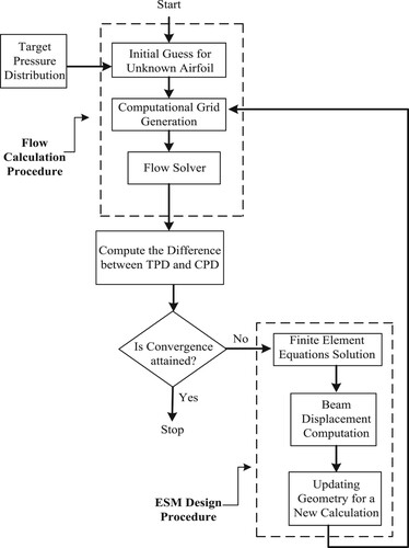
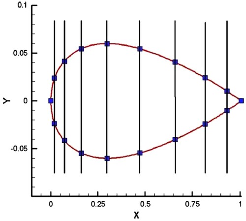
Figure 1 presents a 2D airfoil’s upper wall, which was modelled by an elastic beam. If the difference between the target and computed pressure distributions, as a force distribution, is applied to a flexible beam, it will deform to reach a stationary shape, in which the internal stresses counteract the pressure differences. If the internal stresses inside the beam are set virtually to zero at the beginning of each geometry correction, the flexible beam finally reaches the target geometry, in which the pressure differences approach zero. This model is considered for the lower wall of the airfoil for the ESA inverse design process. In the ESA, the airfoil walls are modelled as two curved beams hinged at both ends (Figure 1). Therefore, the chord length of the airfoil is fixed through geometry corrections. A non-linear finite element method, which was implemented using a FORTRAN code, computes the nodal displacements of the elastic beam at each geometry correction. Figure 2 presents the ESA inverse design procedure.

Figure 1. Modelling a 2D airfoil with two elastic curved beams hinged at both ends in the ESA, only the upper beam is shown.

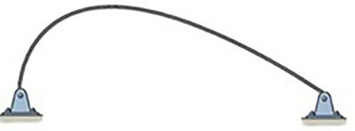
Figure 2. Flowchart of the ESA inverse design process.

3. Beam finite element model based on Timoshenko theory

As mentioned before, the ESA solves the large deformation equations of a curved beam using a nonlinear finite-element method based on the Timoshenko theory developed by Felippa [47]. In this method, the curved beam is divided to planar beam elements. Each beam element has two end nodes (Figure 3). As shown in Figure 3, the ith node has three degrees of freedom: $u_{X_i}$ is the displacement of node i in X direction, $u_{Y_i}$ is the displacement of node i in Y direction and ${\mathit{\theta }}_i$ is the rotation of node i.

Figure 3. Two-node beam element with six degrees of freedom [47].

To determine the stiffness matrix of the elements, a displacement vector was first guessed for each beam element Equation (1): (1) $\mathbf{\text{u}}={\left[\begin{array}{ccc}{u}_{X1}& u_{Y1}& {\theta }_1\end{array}\begin{array}{ccc}{u}_{X2}& u_{Y2}& {\theta }_2\end{array}\right]}^T$(1)

The displacement field and displacement gradient of each element were calculated via the above displacement vector. The axial strain, $e$, shear strain, $\gamma$, and curvature, $\kappa$, for each element were then calculated using the element displacement field and displacement gradient (see [47] for more information). Finally, the internal forces of all elements were calculated using the values of the strains: (2) $\begin{array}{rl}N& =N^0+E{A}_{0}e\end{array}$(2) (3) $\begin{array}{rl}V& =V^0+G{A}_0\gamma \end{array}$(3) (4) $\begin{array}{rl}M& =M^0+E{I}_0\kappa \end{array}$(4) where N, V, and M are the axial force, shear force, and bending moment of the element, respectively. The initial values of these forces are marked by the superscript 0, and are equal to zero at each stage of the shape correction process. E is the elasticity modulus and G is the shear modulus of the beam element. $A_0$ is the cross-sectional area and $I_0$ is the moment of inertia of the beam element, which are constant. G, $A_0$ and $I_0$ are calculated as follows: (5) $\begin{array}{rl}G& =\frac{12E{I}_0}{A_0{L}_0^2}\end{array}$(5) (6) $\begin{array}{rl}{A}_0& =bt\end{array}$(6) (7) $\begin{array}{rl}{I}_0& =\frac{b{t}^3}{12}\end{array}$(7)

The shear modulus (G) is calculated by Equation (5) in order to avoid and remove ‘shear locking’. Shear locking is a structural phenomenon that may cause numerical errors in the nonlinear finite element computations.

The strain (internal) energy of the element ($U$) is given by (8) $\delta U={\int }_{L_0}(N\delta e+V\delta \gamma +M\delta \kappa )d\overline{X}$(8) where $\overline{X}$ denotes the beam longitudinal axis in the reference configuration. Then, the internal force vector of the element ($\mathbf{\text{p}}$) is obtained by taking derivative of the strain internal energy with respect to the node displacements: (9) $\delta U={\mathbf{\text{p}}}^T\delta \mathbf{\text{u}}$(9)

The stiffness matrix of the element, ${\mathbf{\text{K}}}_e$, is defined by the first-order changes in the internal force vector: (10) $\delta \mathbf{\text{p}}={\mathbf{\text{K}}}_e\delta \mathbf{\text{u}}$(10) It should be noted that the internal force vector of the element ($\mathbf{\text{p}}$) is an intermediate vector used to compute the element stiffness matrix and does not have a direct application in the inverse design algorithm, unlike the pressure distribution and external force vector (f). Detailed descriptions for calculating the element stiffness matrix (${\mathbf{\text{K}}}_e$) can be found in Ref. [47].

The total stiffness matrix of the curved beam is obtained by the superposition of the stiffness matrices of the elements. The total displacement vector of the curved beam is recalculated by solving the following equation: (11) $\mathbf{\text{K}}({\mathbf{\text{u}}}_B^n){\mathbf{\text{u}}}_B^{n+1}=\mathbf{\text{f}}$(11) where K, ${\mathbf{\text{u}}}_B$, and f are respectively the stiffness matrix and nodal displacement vector of the curved beam, and force vector exerted on the curved beam’s nodes. Also, the superscripts n and n + 1 refer to the current and updated displacement vector, respectively. The positions of all nodes are recalculated by solving Equation (11). The entire process is repeated and the stiffness matrix is recalculated until the vector ${\mathbf{\text{u}}}_B$ converges to a constant vector. Finally, the displacement of the curved beam is obtained.

Moreover in each inverse design iteration, the difference between the target and current pressure distributions is applied to the curved beam as a continuous load distribution. This load distribution is equivalent to a set of 2D force vectors exerted on the curved beam nodes. Each vector is decomposed to X and Y components. All of these X and Y components are aggregated in the external force vector (f) which is used in Equation (11).

4. Numerical solver

In this study, the Reynolds Averaged Navier-Stokes equations (RANS), which describe the conservation of mass, momentum and energy, are solved using a finite volume method at steady flow conditions. The flow is assumed to be two-dimensional, viscous, and incompressible. The discretization of the equations is achieved using the pressure-based implicit method, in which the equations are solved coupled. The second-order upwind discretization scheme is to interpolate the variables stored at the cell centres to the faces. The gradients and derivatives inside the cells are computed from the Least-Square Cell-Based relationship. The SIMPLE algorithm is used for a combination of continuity and momentum equations to derive an equation for a pressure correction. The Reynolds stress terms in the momentum transport equations are resolved using the shear-stress transport (SST) turbulence model, and the compressibility effects are considered for this model. C-type structured grid is considered for the numerical domain that is fine enough near the wall to calculate the wall shear stress distribution with a sufficient precision. Sections 6 and 7 describe the grid size. Also, Table 1 provides details of the numerical solution, numerical grid and boundary conditions for all validation and design cases in Sections 6 and 7.

Table 1. Details of the numerical solution, grid and boundary conditions for the flow field in the ESA.

Inlet and outlet boundary conditions	Velocity	Free stream velocity	68 m/s
Free stream Reynolds number	4.66 × 10^6	Free stream Much number	0.2
Compressibility condition	Incompressible	Free stream density	1.225 kg/m^3
Ambient temperature	15 C	Ambient pressure	1 bar
Turbulence assumption	fully turbulent	Flow equations	RANS
Type of the mesh	C-type Structured	Turbulence model	k-ω-SST
Medium grid resolution	530 × 100	Fine grid resolution	1060 × 200
Number of cells on the airfoil wall for medium grid	120	Number of cells on the airfoil wall for fine grid	240

5. Grid study

In a general CFD analysis, it is necessary to conduct a grid study to find a sufficiently fine grid with reliable aerodynamic coefficients and acceptable wall Y⁺. But, using the fine grid in the CFD analysis, which is used during the inverse design process, will lead to a high computational cost for the inverse design. Therefore, a low-fidelity CFD analysis with a coarse or medium grid size should be used in each geometry correction to have a rapid and robust inverse design process.

The low-fidelity CFD analysis is appropriate for validating the inverse design because the initial and target geometries are already known and the aim is only the validation of the inverse method. However, after performing a design case, the flow only over the initial and final geometries is solved by using a high-fidelity CFD analysis with a sufficiently fine grid size to compare the performances of the initial and target geometries. This strategy decreases the computational cost of the inverse method for the real design cases. In the present study, the grid resolutions of 530 × 100 and 1060 × 200 were used for the low- and high-fidelity CFD analyses, respectively.

To validate the CFD flow solver, the aerodynamic coefficients of NACA0012 airfoil at Re = 6 × 10⁶ were numerically obtained by the CFD solution and compared with the experimental results reported in Ladson [48]. Other numerical solution conditions are the same as Table 1. Moreover, four C-type structured grids with different resolutions and different element ratios were considered for the grid study. The properties of these grids and values of averaged Y⁺ are presented in Table 2.

Table 2. The properties and the averaged values of Y⁺ of four C-type structured grids, used for the numerical solution of NACA0012 airfoil at Re = 6 × 10⁶.

Grid number	Resolution	Successive ratio	Last/first element size ratio	$Y_{\text{averaged}}^{+}$
1	530 × 100	1.06	318	237.2
2	1060 × 150	1.06	5870	13.9
3	1060 × 175	1.06	23,300	3.33
4	1060 × 200	1.06	108,000	0.77

Moreover, the diagrams of lift and drag coefficients versus the grid number for NACA0012 airfoil at Re = 6 × 10⁶ and AOA = 6° are shown in Figures 4 and 5. According to the asymptotic behaviours of Figures 4 and 5 and the values of Y⁺ in Table 2, Grid 4 with Y⁺ < 1 (appropriate for k-ω-SST turbulence model) was chosen for the validation of CFD flow solver with experimental results. The comparison of CFD results and experimental data is accomplished only for the angles of attack before the stall. Figure 6 compares the diagrams of lift and drag coefficients versus the angle of attack (AOA) for the CFD solution and experimental data [48]. As shown in Figure 6, there is a little more difference between drag coefficients than lift coefficients. Some researches such as Eftekhari et al. [49] also reported the same difference between the numerical and experimental drag coefficients in the validation cases of NACA0012 CFD solution. However, according to Figures 4–6 and Table 2, Grid 1 (530 × 100) and Grid 4 (1060 × 200) were considered for the low- and high-fidelity CFD analyses, respectively.

Figure 4. Diagram of drag coefficient versus the grid number for NACA0012 airfoil at Re = 6 × 10⁶ and AOA = 6°.

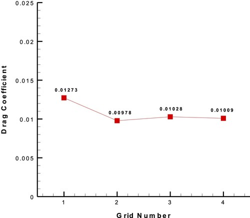
Figure 5. Diagram of lift coefficient versus the grid number for NACA0012 airfoil at Re = 6 × 10⁶ and AOA = 6°.

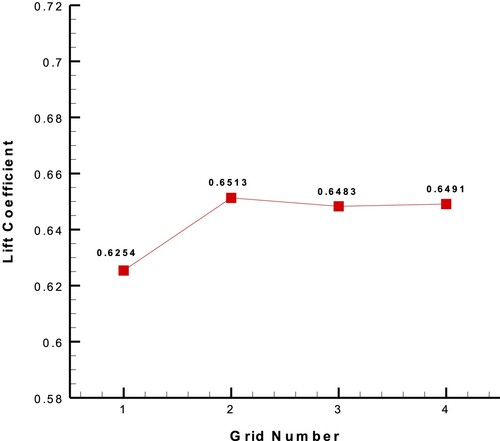
Figure 6. Diagrams of (a) lift coefficient and (b) drag coefficient versus angle of attack, obtained from the CFD solution (with Grid 4) and transition free experimental data reported in Ladson [48].

6. Upgrading the ESA

As explained in Section 2, the original ESA replaces a curved elastic beam instead of the airfoil surface to correct the geometry. The following modifications need to be applied to the original ESA for its upgrade in separated flows.

6.1. Removing geometrical filtrations

The original ESA decreased the convergence accuracy of the FEM equations and used a geometrical filtration for the fractures generated in the geometry to increase the beam displacement in the intermediate geometry corrections. If a continuous load distribution is applied to an elastic beam, the deflection curve of the beam will be continuous and four-times differentiable at all nodes without fracture. By increasing the beam elasticity modulus and decreasing the convergence criterion to 10⁻⁶ for FEM equations, no fracture will be observed in the deformed shape of the airfoil during the geometry corrections. The convergence criterion for FEM equations (the residual of nodal displacements) is expressed in Equation (12): (12) $\text{FEM - RMS}=\sqrt{\sum _{i=1}^{3n}{(\mathrm{\Delta }{\phi }_i^{k+1}-\mathrm{\Delta }{\phi }_i^k)}^2/3n}$(12)

In Equation (12), each node has three degrees of freedom in the x, y, and $\mathit{\theta }$ directions, which are shown by $\phi$. Therefore, if the number of beam nodes is n, the total number of degrees of freedom is 3n.

 Figure 7 presents the residuals of nodal displacements of the beam respectively for the convergence criteria of 10⁻² and 10⁻⁶. According to the figure, some fractures occur in the airfoil shape when the beam finite element equations are not converged completely. To solve the finite-element equations with a convergence criterion of 10⁻⁶, the beam elasticity modulus should be increased. Figure 7b shows the displacement residuals of the FEM equations. As a result, no geometrical filtration is needed for the modified subroutine in the FORTRAN code.

Figure 7. Variations of the displacement residual in the beam finite element equations for (a) convergence criterion of 10⁻², and (b) convergence criterion of 10⁻⁶ (increased elasticity modulus) for the same geometry modification.

6.2. Automatic determination of the beam elasticity modulus from iteration two onward

To achieve the maximum beam displacement at the first geometry correction, the least possible value of E, in which the beam FEM equations can converge with an accuracy of 10⁻⁶, should be considered. Because the difference between the target and current pressure distributions decreases gradually through the geometry corrections, the beam elasticity modulus should also be decreased logically and automatically. This causes a sufficient convergence rate for the inverse design procedure.

The numerical experiences in this study show that if the reduction of E has a linear proportion with the reduction of the difference between the target and current pressures, the convergence rate of ESA improves with no divergence and instability. Equations (13) and (14) show the dimensionless parameter of Q that is assumed to be constant during the inverse design process: (13) $\begin{array}{rl}Q& =\left(\frac{E}{\mathrm{\Delta }{P}_{\text{int}}}\right)\end{array}$(13) (14) $\begin{array}{rl}\mathrm{\Delta }{P}_{\text{int}}& =\int (P_{\text{target}}-P_{\text{current}})d{S}^{\ast }\end{array}$(14)

Here, $\int P_{\text{target}}d{S}^{\ast }$ and $\int P_{\text{current}}d{S}^{\ast }$ are the integrals of the target and the current pressure distributions at each geometry modification step, respectively. Moreover, the value of Q is determined at the beginning of the inverse design process, so that the initial shape pressure distribution ($P_{\text{initial}}$) is replaced with $P_{\text{current}}$ in Equation (14) and the initial value of elasticity modulus ($E_0$) is replaced in Equation (13). It should be noted that the value of $E_0$ depends on the initial geometry and the initial value of hybrid flow parameter ($\mathrm{\Delta }H$) (see Subsection 6.5), so that the value of $E_0$ is case-dependent. Finally, the determined value of Q is considered to be constant during the inverse design process.

6.3. Elimination of vertical spines for node displacement

To solve the large deformation equations of a curved beam (airfoil wall) using the FEM, the curved beam is divided into several elements, which are joined together through the nodes. In the original ESA, as shown in Figure 8, all nodes except the two supports could move freely along the vertical spines ($\mathrm{\Delta }X=0$). This limits the large deformation approach significantly, decreases the beam displacements, and slows down the convergence rate of the inverse design.

Figure 8. Applying the constraint of $\mathrm{\Delta }X=0$ for all nodes on the airfoil surface.

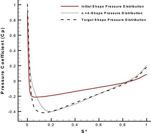
Therefore, the constraint of $\mathrm{\Delta }X=0$ is removed for the upgraded ESA to satisfy the theory of large deformations. Figure 9 shows a validation case that considers NACA0011 as the target geometry and an airfoil with a half thickness as an initially-guessed geometry. According to this figure, by removing the constraint of $\mathrm{\Delta }X=0$, increasing the solution accuracy of the FEM equations, and choosing a sufficient value for the beam elasticity modulus, the airfoil wall has a large extent of deformation at only four geometry corrections. Figure 10 shows that the pressure and shear stress distribution approaches the target quickly.

Figure 9. Large deformations of NACA0011 airfoil wall at the initial geometry corrections after removing the constraint of $\mathrm{\Delta }X=0$ for intermediate nodes.

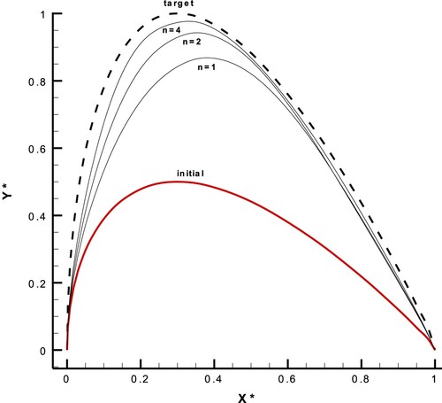
Figure 10. Current pressure distribution being close to the target one after four geometry corrections, by removing the constraint of $\mathrm{\Delta }X=0$ for intermediate nodes.

In the ESA process for some blunt-edged airfoils, despite increasing the beam deformation at the initial geometry corrections, the target shape cannot be achieved at the final geometry corrections because the vertical spine path for the node displacement is removed. Therefore, in these cases, the constraint of $\mathrm{\Delta }X=0$ for all nodes will be returned at the final geometry corrections to achieve the final shape.

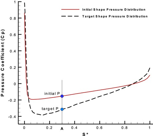
6.4. Description of shape modification algorithm based on dimensionless surface length (S*)

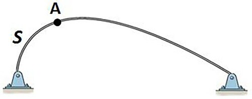
According to Figure 11, if the distance travelled on the airfoil curve from the leading edge to an arbitrary point A is assumed to be S, the dimensionless length of S* is defined as the value of S divided by the total curve length. As explained in Subsection 6.3, the airfoil wall is divided into several elements, which are joined together through the nodes. Each element is assumed as a spline, so the spline equations are used to calculate the curve length and determining the value of S at an arbitrary point.

Figure 11. Schematic view of S-coordinate on the airfoil wall.

The shape modification algorithm based on the dimensionless surface length (S*) is described as follows:

1. The curved beam of the initial airfoil is divided into several beam elements, which are joined together through the nodes. The values of S and S* are calculated for all these nodes. These initial S* values will be fixed through the whole process of inverse design.

2. The CFD simulation of the fluid flow around the initial airfoil is carried out to calculate the corresponding wall pressure distribution versus S and then S* (but not X).

3. The initial S* values intersect with the diagram of target pressure distribution to interpolate the target pressure values at the same S* values of the initial pressure (Figure 12).

4. The difference between the target and initial pressure values at the initial S* values (with details explained in steps 4 and 5) is applied to the initial airfoil wall to deform it. Both leading and trailing Edges are hinged, and the constraint of $\mathrm{\Delta }X=0$ is removed for the intermediate nodes (see Subsection 6.3).

5. The new values of S are calculated for the nodes on the new deformed wall, and the CFD calculates the corresponding wall pressure distribution versus the new S. Also, the internal stresses created in the deformed wall are virtually set to zero for the next shape modification step.

6. The initial S* values intersects with the new computed pressure distribution to interpolate the computed pressure values at the same initial S* values (Figure 12).

7. Steps 4–6 are repeated until the current pressure distribution converges to the target one.

Figure 12. Comparing the initial (current) and target pressures at the same S* for an arbitrary node.

6.5. Applying the wall shear stress distribution

In the geometry correction cases with separation, the pressure distribution is not sensitive to variations in geometry, so that it is impossible to use only the pressure distribution for the shape modification. Because the pressure inside the separation zone over the suction side of a blunt-leading-edged airfoil is almost constant, the use of pressure as the target parameter for the inverse design cases with separation causes very slow convergence, divergence or a non-unique answer. On the other hand, the wall shear stress distribution is sufficiently sensitive to the geometry variations in the separation zone. Therefore, it is necessary to define a hybrid target-flow parameter as a linear combination of the shear stress and pressure distributions for these cases Equation (15). (15) $\mathrm{\Delta }H=\alpha (P_{\text{target}}^{\ast }-P_{\text{iteration}}^{\ast })+\beta ({\tau }_{\text{target}}^{\ast }-{\tau }_{\text{iteration}}^{\ast })$(15) where $\mathrm{\Delta }H$ is the hybrid flow parameter, in which both the pressure and shear stress differences are normalized. Therefore, the force distribution, which is applied perpendicular to the wall, is obtained from the linear combination of the normalized pressure differences and the normalized shear stress differences in Equation (15).

For external flows without separation, the wall shear stress decreases when wall pressure increases and vice versa.

The pressure inside the boundary layer does not change and is almost equal to that on the boundary layer edge. For a positive pressure gradient, the free-stream velocity along the boundary layer edge decreases. The positive pressure gradient also increases the rate of growth of the boundary layer thickness. Both two reasons decrease the velocity gradient normal to the wall ($\mathrm{\partial }V/\mathrm{\partial }n$). As a result, the wall shear stress decreases.

For negative pressure gradient, the free-stream velocity along the boundary layer edge increases, which decreases or prevents the rate of growth of the boundary layer thickness. This causes the velocity gradient normal to the wall ($\mathrm{\partial }V/\mathrm{\partial }n$) to increase, which increases the wall shear stress. It indicates that the slope of wall pressure and shear stress distributions are opposite.

Flesch et al. [50] presented the following correlation for the incompressible turbulent boundary layer with pressure gradient: (16) $C_f\approx 0.058R{e}_{\theta }^{-0.268}(0.93-1.95{\log }_{10}H{)}^{1.705}$(16)

Although the above correlation can predict the onset of separation ($C_f=0$ at $H=3.0$), it is not able to model the turbulent separated region. By simplifying Equation (16), the following correlation is derived: (17) ${\tau }_w\approx A_1{U}_e^{1.732}{\theta }^{-0.268}$(17) where $A_1$ is as follows: (18) $A_1=0.029\rho {\nu }^{0.268}(0.93-1.95{\log }_{10}H{)}^{1.705}$(18) where the shape factor (H) is assumed to be approximately constant. Thus, the parameter $A_1$ is almost constant. Because the flow is incompressible, the Bernoulli Equation can be used along on the boundary layer edge as follows: (19) $P_0=P+\frac{1}{2}\rho U_e^2$(19) where total pressure ($P_0$) is constant outside the boundary layer. By combining Equations (17)–(19), the following correlation between wall pressure, wall shear stress, and momentum thickness is obtained for non-separated flows: (20) $P\approx P_0-A_3{\tau }_w^{1.155}{\theta }^{0.31}$(20) where $A_3$ is: (21) $A_3=\frac{29.82}{{\rho }^{0.155}{\nu }^{0.31}{(0.93-1.95{\log }_{10}H)}^{1.97}}$(21)

The parameter $A_3$ like $A_1$ is assumed to be approximately constant. Also in a Newtonian fluid flow without separation, the variations of momentum thickness are less than the variations of pressure and shear stress [51,52]. According to Equation (20), the power of momentum thickness ($\theta$) is 0.31 while the power of wall shear stress (${\tau }_w$) is 1.155. It means that the variation of the momentum thickness is less than that of the wall shear stress. On the other hand, the power of shear stress is 1.155 that is close to 1. As a result, by differentiating from Equation (20), the following approximate correlation is obtained. (22) $\frac{\mathrm{\partial }P}{\mathrm{\partial }S}\propto -\frac{\mathrm{\partial }\tau }{\mathrm{\partial }S}$(22)

In the original ESA, the target and current pressure distributions are applied to the airfoil wall from the outer and inner side of the airfoil, respectively, according to Figure 13. By defining the dimensionless variable of surface length (S*) in Subsection 6.4, the target and the current pressures are applied perpendicular to the airfoil wall at each point. The target and the current shear stresses are also applied perpendicular to the airfoil wall at each point. Because the wall pressure gradient at each node is approximately proportional to the symmetry of the wall shear stress gradient, the direction of applying shear stress differences and pressure differences are opposite (Figure 14).

Figure 13. How to apply target and current pressure distributions to the airfoil wall in the ESA.

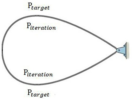
Figure 14. How to apply target and current shear stress distributions to the airfoil wall in the ESA.

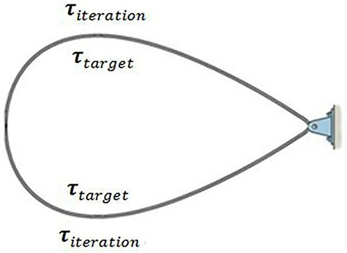
According to the above description, the $\alpha$ and $\beta$ coefficients in Equation (15) should be set to 1 and −1, respectively, so the hybrid flow parameter will be the same as Equation (23): (23) $\mathrm{\Delta }H=(P_{\text{target}}^{\ast }-P_{\text{iteration}}^{\ast })-({\tau }_{\text{target}}^{\ast }-{\tau }_{\text{iteration}}^{\ast })$(23)

It should be noticed that the shear stress difference is far smaller than the pressure difference. So, both the pressure and shear stress differences should be normalized to have the same order of magnitude Equations (24) and (25): (24) $\begin{array}{rl}{P}_{\text{target}}^{\ast }-P_{\text{iteration}}^{\ast }& =\frac{P_{\text{target}}-P_{\text{iteration}}}{P_{\text{target,max}}-P_{\text{target,min}}}\end{array}$(24) (25) $\begin{array}{rl}{\tau }_{\text{target}}^{\ast }-{\tau }_{\text{iteration}}^{\ast }& =\frac{{\tau }_{\text{target}}-{\tau }_{\text{iteration}}}{{\tau }_{\text{target,max}}-{\tau }_{\text{target,min}}}\end{array}$(25) where $P_{\text{target,max}}$ and $P_{\text{target,min}}$ are the maximum and minimum values of the target pressure distribution, respectively. Also, ${\tau }_{\text{target,max}}$ and ${\tau }_{\text{target,min}}$ are the maximum and minimum values of the target shear stress distribution, respectively. Therefore, both normalized pressure and shear stress differences have the same scale in Equation (23) so that the shear stress difference affects the geometry correction as much as the pressure difference during the inverse design process.

In this research, the parameter $\mathrm{\Delta }H$ Equation (23) was obtained from the correlation of non-separated flows Equation (16). However, the pressure is almost constant along and across a separation region and the pressure distribution is not sensitive to the geometry variations near the separation zone. Thus, the term of pressure difference in Equation (23) becomes negligible and the parameter $\mathrm{\Delta }H$ almost includes the term of shear stress difference. Therefore, the parameter $\mathrm{\Delta }H$ can be applied for the inverse design of non-separated flows (Subsection 7.1) and flows with separation (Subsections 7.2, 7.3, 8.1 and 8.2).

7. Validation of the upgraded ESA

To validate the inverse design method, a known geometry is assumed as the target geometry, and the corresponding pressure or shear stress distribution is considered as the target pressure or shear stress distribution. An arbitrary geometry is then considered as the initially-guessed geometry. The inverse design method is correctly verified if the initial pressure or shear stress distribution converges to the target pressure or shear stress distribution, and the initially-guessed geometry converges to the target geometry. To evaluate the robustness of the upgraded ESA, two different airfoils are chosen for validation: a symmetrical airfoil (NACA0011) and an asymmetric airfoil (FX63-137). For all validation cases, the inverse design procedure is carried out based on the hybrid target flow parameter Equation (15), including both the pressure and shear stress distributions.

7.1. NACA0011 with AOA = 0

The symmetrical NACA0011 airfoil was assumed as the first target geometry, and the angle of attack (AOA) was set to zero. As expected, the flow field over the airfoil was symmetrical, and there was no separation on the airfoil walls. For grid generation, the C-type structured grid, as shown in Figure 15, was used, and low-fidelity grid resolution was $530\times 100.$

Figure 15. C-type structured Grid 1 over NACA0011 airfoil for low-fidelity CFD analysis.

The k-ω-SST turbulence model was used in this validation case. The chord length of the airfoil was one, and it was constant during the geometry corrections. Both sides of the airfoil were modified separately, and the number of elements on each side was 29.

Safari et al. [44] completely validated the original ESA for a NACA0011 airfoil at AOA = 0 without separation. The target function was the pressure distribution at that work. To check the effect of pressure and shear stress together on the inverse design process, the hybrid flow parameter, which was defined in Equation (15), was considered as the target parameter in this case. One-half thickness of NACA0011 was considered as the initially-guessed geometry.

The coefficients, $\alpha$ and $\beta$, were set to 1 and −1, respectively. At the final steps of geometry correction (from iteration 130 onward), when the current geometry was close to the target geometry, the shear stress distribution was not sensitive to variations in geometry. Therefore, the $\beta$ coefficient was set to zero. Figures 16–19 present the results of this validation after 318 geometry corrections.

Figure 16. Geometry correction for a NACA0011 airfoil with AOA = 0 considering the hybrid target flow parameter.

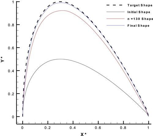
Figure 17. Shear stress distributions for the initial, target, and final shapes, in the case of a NACA0011 airfoil with AOA = 0 considering the hybrid target flow parameter.

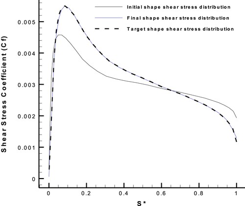
Figure 18. Pressure distributions for the initial, target, and final shapes, in the case of a NACA0011 airfoil with AOA = 0 considering the hybrid target flow parameter.

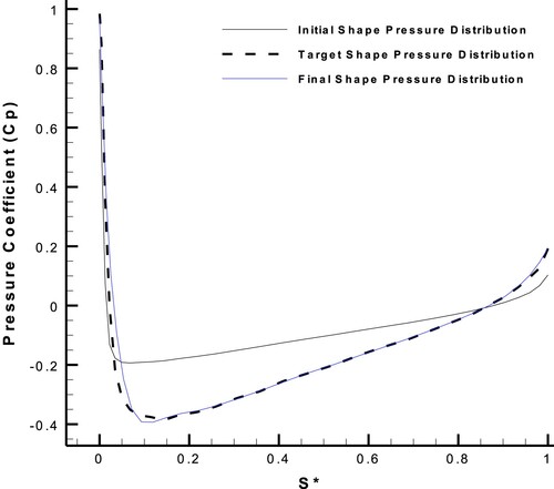
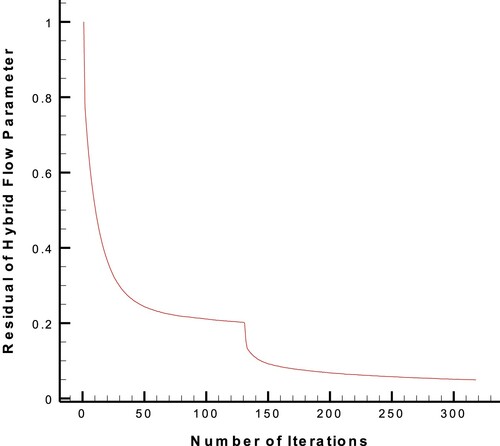
Figure 19. Convergence of the hybrid flow parameter residual through geometry modifications of NACA0011 airfoil with AOA=0.

In this paper, all diagrams are presented by non-dimensional quantities including X*, Y* and S* coordinates, pressure coefficient (C_p), and shear stress coefficient (C_f). These non-dimensional quantities are defined as follow: (26) $\begin{array}{rl}{X}^{\ast }& =\frac{X}{C},Y^{\ast }=\frac{Y}{T_{\text{target,max}}},S^{\ast }=\frac{S}{S_{\text{total}}}\end{array}$(26) (27) $\begin{array}{rl}{C}_P& =\frac{P-P_{\text{inf}}}{\frac{1}{2}{\rho }_{\text{inf}}{U}_{\text{inf}}^2},C_f=\frac{{\tau }_w}{\frac{1}{2}{\rho }_{\text{inf}}{U}_{\text{inf}}^2}\end{array}$(27) where $C$ and $S_{\text{total}}$ are the chord length and total curve length of the airfoil, respectively. $T_{\text{target,max}}$ is the maximum thickness of the target shape. Also, ${\rho }_{\text{inf}}$, $P_{\text{inf}}$ and $U_{\text{inf}}$ are the density, pressure and velocity of the free stream fluid, which are presented in Table 1.

Moreover, as shown in Figure 19, there is a jump in the diagram at iteration 130. The reason is the change of $\beta$-value from −1 to 0 at iteration 130.

7.2. NACA0011 with $\text{AOA}=6^{\circ }$

If the NACA0011 airfoil at AOA = $6^{\circ }$ is assumed as the target geometry, the flow over the whole airfoil will be asymmetric as shown in Figure 20. The numerical grid was the same as used in Subsection 7.1 (Figure 15) and the low-fidelity grid resolution was $530\times 100$. The turbulence model was k-ω-SST, either.

The results showed that the chord length of the airfoil was one, and it remained constant during the inverse design process. Only the suction side of the airfoil (upper wall) was deformed, and the pressure side (lower wall) was fixed. The number of elements on the suction side beam was 29.

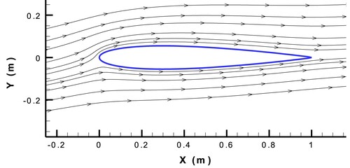
Figure 20. Streamlines showing the asymmetric flow over NACA0011 airfoil with AOA = $6^{\circ }$ obtained by the numerical solution with k-ω-SST turbulence model.

The same as Subsection 7.1, the coefficients, $\alpha$ and $\beta$, were set to 1 and −1, respectively, to check the effect of pressure and shear stress together on the inverse design of external flows with separation. Figures 21–23 present the results of this validation after 65 geometry corrections.

Figure 21. Geometry modification process for the suction side of a NACA0011 airfoil with AOA = $6^{\circ }$, considering the hybrid target flow parameter.

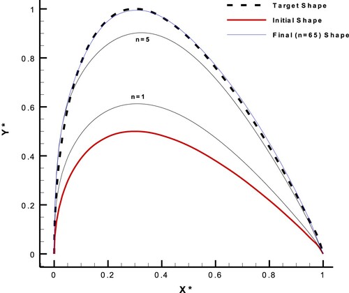
Figure 22. Initial, target and final shear stress distributions on the suction side of NACA0011 airfoil with AOA = $6^{\circ }$, considering the hybrid target flow parameter.

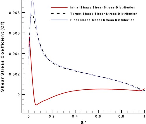
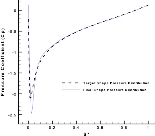
Figure 23. Target and final pressure distributions on the suction side of NACA0011 airfoil with AOA = $6^{\circ }$, considering the hybrid target flow parameter.

According to Figure 22, shear stress is negative near the leading edge of the initial shape, which indicates a large LE separation. This is while the shear stress distributions of the target and final shapes are thoroughly positive, which means no separation. Streamlines near the leading edge of initial and target airfoils are shown in Figure 24 (final airfoil was ignored, because its geometry had been converged to the target one):

Figure 24. Contours of streamlines near the LE of initial and target (NACA0011) airfoils with AOA = $6^{\circ }.$

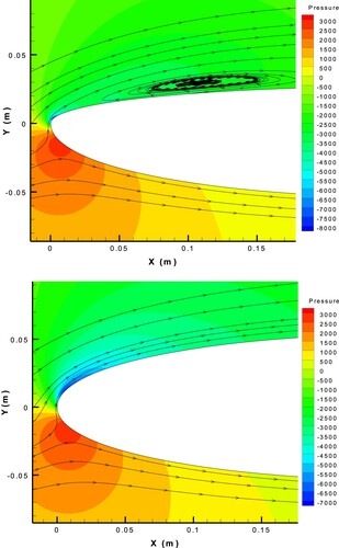
Although Subsection 7.2 is a validation case, it shows the ESA inverse design method to be capable of changing the flow (and geometry) of an airfoil with LE separation to an airfoil with no separation (Figure 24). From practical side, this case can be useful for the design goals.

Moreover, lift ($C_l$), pressure drag ($C_{d\mathbf{\text{P}}}$), friction drag ($C_{d\mathbf{\text{F}}}$) and total drag coefficients ($C_d$) were calculated with high-fidelity CFD analysis for the initial and final airfoils and shown in Table 3 (The target airfoil was ignored, because the final airfoil had been converged to the target one):

Table 3. Lift and drag coefficients of the initial and final airfoils, in the validation case of NACA0011 with AOA = $6^{\circ }.$

	$C_{d\mathbf{\text{P}}}$	$C_{d\mathbf{\text{F}}}$	$C_d$	$C_l$	$C_l/C_d$
Initial Shape	0.0280	0.0037	0.0317	0.417	13.133
Final Airfoil	0.0077	0.0056	0.0134	0.605	45.293
Percentage (%) of variations during design process	−72.5	51.4	−57.7	45.1	245

As shown in Table 3, although the friction drag coefficient increases, the total drag coefficient decreases during the design process, which leads to a significant increase of the lift coefficient and lift-to-drag ratio. This case shows how the ESA can be used for the airfoil performance improvement by eliminating the separation zone using shear stress distribution as the target function.

7.3. FX63-137 with $\text{AOA}={10}^{\circ }$, only suction side

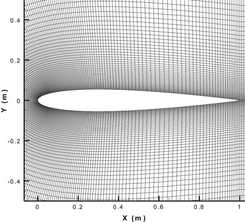
If an asymmetric airfoil, such as FX63-137, at AOA = ${10}^{\circ }$ is assumed as the target geometry, the flow field over the airfoil will be asymmetric and there will be a separation zone on the suction side (upper wall) of the airfoil (Figure 25). For grid generation, a C-type structured grid was used, as shown in Figure 26, and the low-fidelity grid resolution was $530\times 100$. In addition, the turbulence model was k-ω-SST.

Figure 25. Pressure contour and streamlines showing the separation zone on the suction side of the FX63-137 airfoil with AOA = ${10}^{\circ }$ and the k-ω-SST turbulence model.

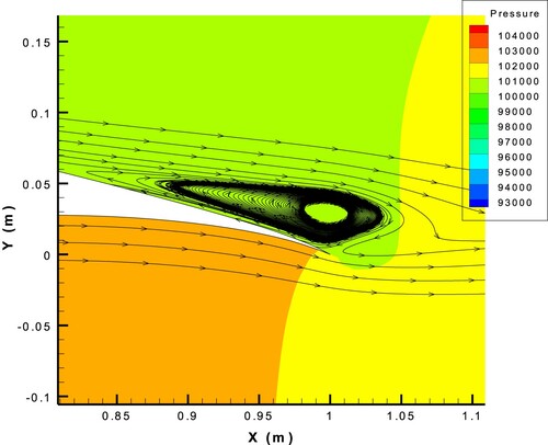
Figure 26. C-type structured Grid 1 over FX63-137 airfoil for low-fidelity CFD analysis.

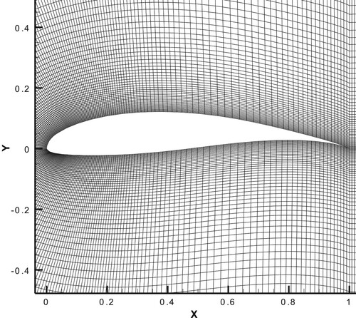
The chord length of the airfoil was one, and it remained constant during the inverse design procedure. In addition, only the suction side (upper wall) of the airfoil was modified, and the pressure side (lower wall) had no deformation. The number of elements on the suction side was 48.

As before, the inverse design process was divided into two levels. At the first level, the $\alpha$ and $\beta$ coefficients were set to 0 and −1, respectively so that the shear stress was the target function. The first level was applied until iteration 26. At the second level, when the current geometry was close to the target one, the $\alpha$ and $\beta$ coefficients were set to 1 and 0, respectively, and the pressure was the target function. 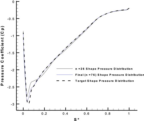In addition, the constraint, $\mathrm{\Delta }X=0$, for the intermediate nodes was applied again. The second level was applied until iteration 76. Figures 27–29 show the results of this inverse design process. Figure 28 shows the variation of shear stress distribution at the first level, and Figure 29 shows the variation of pressure distribution of this inverse design process at the second level.

Figure 27. Geometry modification process for the suction side of the FX63-137 airfoil with AOA = ${10}^{\circ }$, at the 1st and 2nd levels of the inverse design validation.

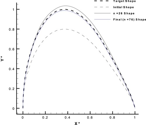
Figure 28. Variation of the shear stress distribution on the suction side of the FX63-137 airfoil with AOA = ${10}^{\circ }$, at the 1st level of inverse design validation.

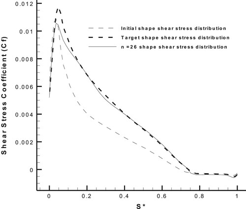
Figure 29. Variation of the pressure distribution on the suction side of the FX63-137 airfoil with AOA = ${10}^{\circ }$, at the 2nd level of inverse design validation.

8. Design

For the aerodynamic design of an airfoil, the existing geometry is considered as the initial guess and its corresponding pressure or shear stress distribution is modified and corrected to be considered as the target pressure or shear stress distribution. During the inverse design procedure, the modified pressure or shear stress distribution should be achieved for the design to be completed. Here, two asymmetric airfoils were redesigned in order to reduce the size of separation zone over their suction side or completely eliminate it.

8.1. FX63-137 with $\text{AOA}={10}^{\circ }$, reducing the separation size over the suction side

For the first design case, the FX63-137 airfoil with AOA = ${10}^{\circ }$ was modified in a way that the separation zone over the suction side was transferred downstream, and its size was reduced so that the airfoil drag force would decrease. The coefficients of $\alpha$ and $\beta$ were set to 0 and −1, respectively. Therefore, only the shear stress distribution on the suction side was modified to be considered as the target function and there was no need for pressure application.

For grid generation, the C-type structured grid was the same as in Figure 26 and the low-fidelity grid resolution was $530\times 100$. Also the number of grid cells on each side of the airfoil was 120.

The chord length of the airfoil had the constant value of one, and only the suction side was deformed. The number of finite beam elements (for shape modification) on the suction side was 48. Figures 30–32 show the results of the inverse design process after 80 evolution steps.

Figure 30. Geometry modification for the suction side of the FX63-137 airfoil with AOA = ${10}^{\circ }$, in the design process with the upgraded ESA.

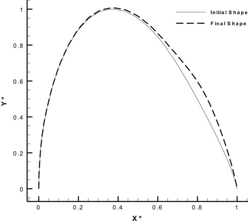
Figure 31. Initial, target, and final shear stress distributions on the suction side of the FX63-137 airfoil with AOA = ${10}^{\circ }$, in the design process with the upgraded ESA.

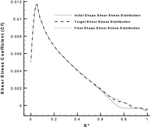
Figure 32. Convergence of shear stress residual through the geometry modifications of the suction side of the FX63-137 airfoil with AOA = ${10}^{\circ }$, in the design process with the upgraded ESA.

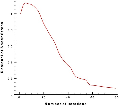
In addition, Figure 33 compares the location, size, and length of the separation zone on the suction side of the airfoil before and after inverse design.

Figure 33. Pressure contour and streamlines showing the separation zone on the suction side of FX63-137 airfoil with AOA = ${10}^{\circ }$ before and after inverse design.

According to Figures 31 and 33, the upgraded ESA with the hybrid target flow parameter in the inverse design of an airfoil with a separated flow could transfer the separation zone downstream the airfoil and reduce its length and size to decrease the airfoil drag force.

Moreover, lift and drag coefficients were calculated with high-fidelity CFD analysis for the initial and final airfoils, and were listed in Table 4.

Table 4. Lift and drag coefficients of the initial and final airfoils, in the design case of FX63-137 with AOA = ${10}^{\circ }.$

	$C_{d\mathbf{\text{P}}}$	$C_{d\mathbf{\text{F}}}$	$C_d$	$C_l$	$C_l/C_d$
Initial Shape	0.0307	0.0054	0.0361	1.6784	46.448
Final Airfoil	0.0287	0.0056	0.0343	1.6926	49.334
Percentage (%) of variations during design process	−6.5	3.7	−5	0.85	6.2

According to Table 4, this design process did not have a great influence on the lift coefficient, but it caused decreasing of the drag coefficient and therefore increasing of the lift-to-drag ratio.

8.2. New airfoil with $\text{AOA}=7^{\circ }$, eliminating the separation zone over the suction side

For the second design case, a new airfoil was considered so that the suction side (upper wall) was the same as NACA0004 and the pressure side (lower wall) was the same as NACA0011. The angle of attack was set to $7^{\circ }$ and the flow field was asymmetric, so that a large separation zone was created over the airfoil suction side.

This new airfoil was modified in a way that the separation zone over the suction side was completely eliminated so that the airfoil drag force would decrease to a large extent. The coefficients of $\alpha$ and $\beta$ were set to 1 and −1, respectively. Therefore, both the pressure and shear stress distributions on the suction side were modified and the hybrid flow parameter was considered as the target function.

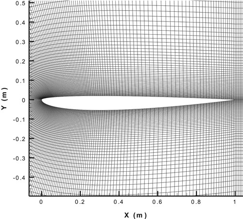
For grid generation, the C-type structured grid was shown in Figure 34 and the low-fidelity grid resolution was $530\times 100$. Also the number of grid cells on each side of the airfoil was 120.

Figure 34. C-type structured Grid 1 over the new airfoil (upper wall the same as NACA0004 and lower wall the same as NACA0011), used for the low-fidelity CFD analysis.

The chord length of the airfoil had the constant value of one, and only the suction side was deformed. The number of finite beam elements (for shape modification) on the suction side was 29. The corresponding pressure and shear stress distributions of NACA0011 with $\text{AOA}=7^{\circ }$ (on the suction side) were considered as the target pressure and shear stress distributions. Figures 35–38 show the results of the inverse design process after 183 evolution steps.

Figure 35. Geometry modification for the suction side of the new airfoil with AOA = $7^{\circ }$, in the design process with the upgraded ESA.

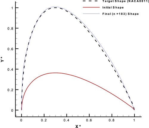
Figure 36. Initial, target, and final shear stress distributions on the suction side of the new airfoil with AOA = $7^{\circ }$, in the design process with the upgraded ESA.

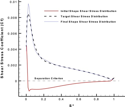
Figure 37. Initial, target, and final pressure distributions on the suction side of the new airfoil with AOA = $7^{\circ }$, in the design process with the upgraded ESA.

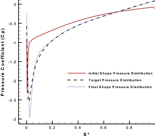
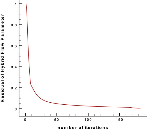
Figure 38. Convergence of hybrid flow parameter residual through the geometry modifications of the suction side of the new airfoil with AOA = $7^{\circ }$, in the design process with the upgraded ESA.

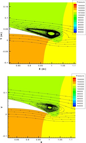
Moreover, Figure 39 compares the streamlines over the airfoil before and after inverse design.

Figure 39. Pressure contour and streamlines over the new airfoil with AOA = $7^{\circ }$ before inverse design (with separation) and after inverse design (without separation).

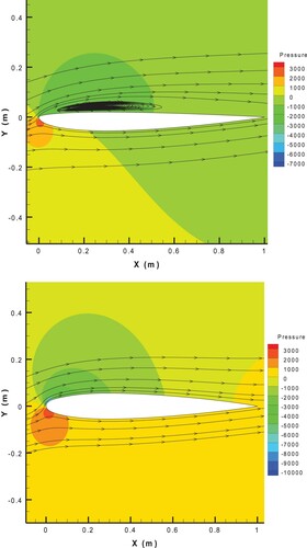
According to Figures 36 and 39, the upgraded ESA with the hybrid target flow parameter completely eliminates the separation zone. Due to the large separation zone in this case, the number of geometry corrections is more than that in the Subsections 7.2, 7.3 and 8.1. Also according to Figures 36 and 37, the normalized difference between the target and initial shear stress distributions is much more than the normalized difference between the target and initial pressure distributions, because of being a large separation zone over the suction side. So, the old inverse design process using only the pressure distribution will cause a very slow convergence rate that is not affordable. Therefore, the shear stress difference should be applied besides the pressure difference in order to attain a rational convergence rate in this design case. Lift and drag coefficients were calculated with the high-fidelity CFD analysis for the initial and final airfoils, which were listed in Table 5.

Table 5. Lift and drag coefficients of the initial and final airfoils, in the design case of new airfoil with AOA = $7^{\circ }.$

	$C_{d\mathbf{\text{P}}}$	$C_{d\mathbf{\text{F}}}$	$C_d$	$C_l$	$C_l/C_d$
Initial Shape	0.0597	0.0029	0.0626	0.4278	6.835
Final Airfoil	0.0107	0.0053	0.0160	0.6988	43.570
Percentage (%) of variations during design process	−82.1	82.8	−74.4	63.35	537.5

As shown in Table 5, although increasing the friction drag coefficient during the design process, the pressure and total drag coefficients decrease and the lift and lift-to-drag ratio increase to a very large extent. Therefore, this inverse design method was able to improve the aerodynamic performance of the airfoil, besides eliminating the large separation zone over the suction side.

8. Conclusion

The main goal of this study was to develop the ESA for the inverse design of blunt-leading-edged airfoils with a separated flow by considering the wall shear stress distribution besides the pressure distribution as the target function. Because the original ESA had been subjected to oscillation instability and divergence for the external flows with separation, the following modifications were applied to the original ESA to upgrade the algorithm:

• The finite element equations were solved numerically with high accuracy to obtain a differentiable deflection curve at all nodes, instead of using geometrical filtrations for the removal of fractures.

• The beam elasticity modulus was determined automatically.

• To increase the beam deformation at each geometry correction, the vertical spines were substituted with the dynamic spines for node displacements.

• A linear combination of the normalized pressure and shear stress distribution as the target flow parameter was considered for the inverse design in separated flow.

The upgraded ESA was then validated for two different blunt-leading-edged airfoils in a subsonic incompressible turbulent flow regime with and without separation. Finally, the aforementioned method was used to redesign the suction side of the FX63-137 airfoil with flow separation. The shear stress distribution was modified to postpone the separation downstream to reduce the drag force and length and size of the separation region.

Although the capability of the upgraded ESA was proved for using the shear stress besides the pressure as the target for external separated flows, it is difficult to define the target pressure and shear stress distributions simultaneously. By the way, this study was the first step in developing this approach in terms of the practical side, and it is required to develop a procedure to define combined distributions of both variables in the future works.

Disclosure statement

No potential conflict of interest was reported by the author(s).

Additional information

Funding

This study was supported by the Brain Pool Program through the National Research Foundation of Korea (NRF) funded by the Ministry of Science and ICT [grant number NRF-2019H1D3A2A01061428]. This work was also supported by the National Research Foundation of Korea (NRF) grant, which is funded by the Korean government (MSIT) [grant number 2020R1A5A8018822].

References

- Jahangirian A, Shahrokhi A. Inverse design of transonic airfoils using genetic algorithm and a new parametric shape method. Inverse Probl Sci Eng. 2009;17:681–699.
- Matsushima K, Takanashi S. An inverse design method for wings using integral equations and Its Recent progress. In: K Fujii, GS Dulikravich, editors. Recent development of aerodynamic design methodologies: inverse design and optimization. Braunschweig/Wiesbaden: Springer Vieweg; 1999. p. 179–209.
- Hajilouy-Benisi A, Nili-Ahmadabadi M, Durali M, et al. Duct design in subsonic and supersonic flow regimes with and without normal shock waves using flexible string algorithm. Scientia Iranica. 2010;17(3):179-193.
- Dulikravich G, Baker D. Aerodynamic shape inverse design using a Fourier series method, in AIAA 99-0185; 1999.
- Ashrafizadeh A, Raithby GD, Stubley GD. Direct design of airfoil shape with a prescribed surface pressure. Numer Heat Trans Part B: Fund. 2004;46(6):505–527.
- Ashrafizadeh A, Raithby G. Direct design solution of the elliptic grid generation equations. Numer Heat Trans Part B: Fund. 2006;50(3):217–230.
- Stanitz JD. Design of two-dimensional channels with prescribed velocity distributions along the channel walls, SEE NACA-TN-2593; NACA-TN-2595, 1952.
- Stanitz JD. Aerodynamic design of efficient two-dimensional channels. Trans ASME. 1953;M. P. No. 52-A-110:1241–1255.
- Stanitz JD. General design method for three-dimensional potential flow fields. NASA Contractor Report 3288; 1980.
- Stanitz JD. A review of certain inverse methods for the design of ducts with 2- or 3-dimensional potential flow. Appl Mech Rev. 1988;41(6):217–238.
- Zannetti L. A natural formulation for the solution of two-dimensional or axisymmetric inverse problems. Int J Numer Methods Eng. 1986;22(2):451–463.
- Ashrafizadeh A, Alinia B, Mayeli P. A new co-located pressure-based discretization method for the numerical solution of incompressible Navier-Stokes equations. Numer Heat Trans Part B: Fund. 2015;67(6):563–589.
- Nikfar M, Ashrafizadeh A. A coupled element-based finite-volume method for the solution of incompressible Navier-Stokes equations. Numer Heat Trans Part B: Fund. 2016;69(5):447–472.
- Nili-Ahmadabadi M, Durali M, Hajilouy-Benisi A, et al. Inverse design of 2-D subsonic ducts using flexible string algorithm. Inverse Probl Sci Eng. 2009;17(8):1037–1057.
- Nili-Ahmadabadi M, Hajilouy-Benisi A, Ghadak F, et al. A novel 2D incompressible viscous inverse design method for internal flows using flexible string algorithm. J Fluids Eng. 2010;132(3):031401.
- Madadi A. 3D-dimensional ball-spine algorithm for determining the profile of an axial flow compressor with specified pressure distribution [PhD thesis]. Mechanical Engineering, Amir Kabir University of Technology; 2014.
- Dulikravich G. Aerodynamic shape design and optimization: status and trends. AIAA J Aircraft. 1992;29(5):1020–1026.
- Dulikravich G. Shape inverse design and optimization for three-dimensional aerodynamics. AIAA invited paper 95-0695, AIAA aerospace sciences meeting, Reno, NV; 1995.
- Dulikravich G. Design and optimization tools development, chapters no. 10–15. In: H Sobieczky, editor. New design concepts for high speed air transport. Wien/New York: Springer; 1997. p. 159–236.
- Garabedian P, McFadden G. Computational fluid dynamics of airfoils and wings. In: RE Meyer, editor. Transonic, shock, and multidimensional flows. New York: Academic Press; 1982. p. 1–16.
- Garabedian P, McFadden G. Design of supercritical swept wings. AIAA J. 1982;20(3):289–291.
- Malone J, Sankar L, Vadyak J. Inverse aerodynamic design method for aircraft components. J Aircr. 1987;24:8–9.
- Malone J, Vadyak J, Sankar L. A technique for the inverse aerodynamic design of nacelles and wing configurations. AIAA Pap.1985;AIAA-85-4096:1-9 .
- Malone J, Narramore J, Sankar L. Airfoil design method using the Navier-Stokes equations. J Aircr. 1991;28(3):216–224.
- Dulikravich G, Baker DP.. Fourier series analytical solution for inverse design of aerodynamic shapes. In: Tanaka M, Dulikravich GS, editors. Inverse problems in mechanics (ISIP '98). Nagano City, Japan: Elsevier Science, Ltd.; 1998. p. 427–436.
- Thinsurat K. Inverse design of airfoils using a flexible membrane method [Master thesis]. University of Texas at Arlington; 2010.
- Dulikravich GS, Baker DP. Using existing flow-field analysis codes for inverse design of three-dimensional aerodynamic shapes. In: K Fujii, GS Dulikravich, editor. Recent development of aerodynamic design methodologies: inverse design and optimization. Wiesbaden: Vieweg + Teubner Verlag; 1999. p. 89–112.
- Hazarika N. An efficient inverse method for the design of blended wing-body configurations [PhD thesis]. Georgia Institute of Technology; 1989.
- Teck W, And T, Zangeneh M. A novel 3D inverse method for the design of turbomachinery blades in rotational viscous flow: theory and applications. Task Quart J. 2002;6(1):63–78.
- Rahmati MT. A new Navier-Stokes inverse method based on mass-averaged tangential velocity for blade design. Int J Numer Methods Fluids. 2009;60(3):323–336.
- Nili-Ahmadabadi M, Hajilouy-Benisi A, Durali M, et al. Duct design in subsonic and supersonic flow regimes with and without normal shock wave using flexible string algorithm. Proc ASME Turbo Expo. 2009;7(48883):513–523.
- Nili-Ahmadabadi M, Durali M, Hajilouy A. A novel aerodynamic design method for centrifugal compressor impeller. J Appl Fluid Mech. 2014;7(2):329–344.
- Nili Ahmadabadi M, Poursadegh F. Centrifugal compressor shape modification using a proposed inverse design method. J Mech Sci Technol. 2013;27:713–720.
- Shumal M, Nili-Ahmadabadi M, Shirani E. Development of the ball-spine inverse design algorithm to swirling viscous flow for performance improvement of an axisymmetric bend duct. Aerosp Sci Technol. 2016;52:181–188.
- Poursadegh F, Hajilouy-Benisi A, Nili-Ahmadabadi M. A novel quasi-3D design method for centrifugal compressor impeller on the blade-to-blade plane. Proc ASME Turbo Expo 2010: Power for Land, Sea, and Air. 2011;54679:1155–1162.
- Nili-Ahmadabadi M, Poursadegh F. Centrifugal compressor shape modification using a proposed inverse design method. J Mech Sci Technol. 2013;27(3):713–720.
- Nili-Ahmadabadi M, Ghadak F, Mohammadi M. Subsonic and transonic airfoil inverse design via ball-spine algorithm. Comput Fluids. 2013;84:87–96.
- Madadi A, Kermani MJ, Nili-Ahmadabadi M. Aerodynamic design of S-shaped diffusers using ball–spine inverse design method. J Eng Gas Turbine Power. 2014;136(12):122606–122606-8.
- Madadi A, Kermani MJ, Nili-Ahmadabadi M. Applying the ball-spine algorithm to the design of blunt leading edge airfoils for axial flow compressors. J Mech Sci Technol. 2014;28(11):4517–4526.
- Madadi A, Kermani MJ, Nili-Ahmadabadi M. Application of the ball-spine algorithm to design axial-flow compressor blade. Scientia Iranica. 2014;21(6):1981–1992.
- Madadi A, Kermani MJ, Nili-Ahmadabadi M. Application of an inverse design method to meet a target pressure in axial-flow compressors. Proc ASME Turbo Expo 2011: Power for Land, Sea, and Air. 2011;54679:1315–1322.
- Madadi A, Kermani MJ, Nili-Ahmadabadi M. Three-dimensional design of axial flow compressor blades using the ball-spine algorithm. J Appl Fluid Mech. 2015;8(4):683–691.
- Mayeli P, Nili-Ahmadabadi M, Besharati-Foumani H. Inverse shape design for heat conduction problems via the ball spine algorithm. Numer Heat Trans Part B: Fund. 2016;69(3):249–269.
- Safari M, Nili-Ahmadabadi M, Ghaei A, et al. Inverse design in subsonic and transonic external flow regimes using Elastic Surface Algorithm. Comput Fluids. 2014;102:41–51.
- Nasrazadani SH, Nili-Ahmadabadi M, Noorsalehi MH. Upgrade and development of elastic surface inverse design method for axial compressor cascade with sharp-edged blades. Numer Heat Transf. 2020;77(1):64–86.
- Noorsalehi MH, Nili-Ahmadabadi M, Shirani E. Inverse design of axial-flow compressor blades using elastic surface algorithm in subsonic and transonic flow regimes with separation. Proc ASME Turbo Expo. 2016;GT2016-56717:1-14.
- Felippa C. Nonlinear finite element methods, (ASEN 6107) DAES. Berlin, Heidelberg: Springer-Verlag / Boulder: University of Colorado;2012.
- Ladson CL. Effects of independent variation of Mach and Reynolds numbers on the low-speed aerodynamic characteristics of the NACA 0012 Airfoil Section, NASA TM 4074; 1988.
- Eftekhari S, Al-Obaidi ASM. Investigation of a NACA0012 finite wing aerodynamics at low Reynolds numbers and 0° to 90° angle of attack. J Aerospace Technol Manage. 2019;11:1-11.
- White FM. Viscous fluid flow, 3rd ed., international edition, University of Rhode Island, New York: McGraw-Hill; 2006.
- Ghadimi P, Bakhshandeh Rostami A, Jafarkazemi F. Aerodynamic analysis of the boundary layer region of symmetric airfoils at ground proximity. Aerosp Sci Technol. 2012;17(1):7–20.
- Yayun S, Junqiang B, Jun H, et al. Numerical analysis and optimization of boundary layer suction on airfoils. Chin J Aeronaut. 2015;28(2):357–367.