
 ?Mathematical formulae have been encoded as MathML and are displayed in this HTML version using MathJax in order to improve their display. Uncheck the box to turn MathJax off. This feature requires Javascript. Click on a formula to zoom.
Abstract
In this paper, we study two identification problems related to the mud filtrate invasion phenomenon. We want to determine a parameter (the invasion rate) in the coefficients of the parabolic equation that describes the mud filtrate invasion phenomenon. In the first problem, we determine this parameter starting from the observed values of the mud filtrate dispersion. We reduce the problem to an optimal control problem and prove the existence of the optimal control. In the second problem, we determine the invasion rate imposing the minimum condition of the quantity of mud filtrate that diffuses into the oil reservoir. We also reduce the identification problem to an optimal control problem. We prove the existence of the optimal control and we obtain a simple explicit form of this optimal control. A numerical example is presented for the second problem.
1. Introduction
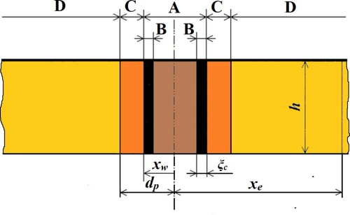
In this paper, we study two identification problems related to the invasion phenomenon arising in the borehole drilling process. During this process the drilling mud is pumped inside of the drill bore (towards the drill bit) and then circulated back to the surface through the annular space between the borehole and the drill bore wall. The drilling mud has sufficiently high density in order to avoid eruptive phenomena so that the hydrostatic pressure of the mud column is higher than the fluid formation pressure. This difference in pressure generates an undesirable phenomenon: the water from the drilling mud (hereinafter referred to as the mud filtrate) invades the formation and radially displaces the hydrocarbons and water from the formation. This invasion alters the reservoir properties in the vicinity of the well bore. The permeability, the porosity and the electrical resistivity of the reservoir are affected. For this reason, the invaded zone is also called the damaged zone.
During the mud filtrate invasion process, a part of the solid particles contained in the drilling mud penetrates the porous medium and another part is deposited on the well wall forming the mudcake. The most used model of the invasion phenomena is the so-called linear single phase mud filtrate invasion model. This model contains two parts:
the mudcake thickness model;
the mud filtrate invasion through the porous media model [Citation1].
a. The mudcake thickness model
Let be the mudcake thickness,
the well radius, h the reservoir (formation) thickness,
the porosity and the mudcake density, respectively, Φ the formation porosity,
the solid particle dispersion in the drilling mud, k and
the reservoir permeability and the mudcake permeability, respectively,
the volumetric flow rate (or invasion rate) (see Figure ). Then, the mudcake growth is described by the following Cauchy problem [Citation1]:
(1)
(1)
(2)
(2) where
(3)
(3)
(4)
(4) and
.
Figure 1. The geometry of the mud-invasion phenomenon. A, wellbore; B, mudcake; C, the invaded zone; D, the drainage zone; , the wellbore radius;
, the drainage radius;
, the mudcake thickness;
, the penetration depth.
From (Equation2(2)
(2) ), (Equation3
(3)
(3) ) and (Equation4
(4)
(4) ) we obtain that
is the maximum value of filtration rate.
b. The mud filtrate dispersion through the porous media model.
In [Citation1], the authors propose the following model in order to determine the mud filtrate dispersion C in the invaded zone:
(5)
(5) for
(6)
(6)
(7)
(7) The mixed problem (Equation5
(5)
(5) )–(Equation7
(7)
(7) ) describes the mud filtrate invasion through the porous media. The initial condition (Equation6
(6)
(6) ) specifies that at t = 0 the mud filtrate dispersion is
In the Dirichlet boundary conditions (Equation7
(7)
(7) ),
represents the mud filtrate dispersion at the wall well. Instead of conditions (Equation7
(7)
(7) ), the Dirichlet–Neumann boundary conditions can also be used [Citation2, p.747]:
(8)
(8) The first term in the right member of Equation (Equation5
(5)
(5) ) is the conductive term. Here D is the diffusion coefficient. Based on experimental results, several authors proposed for D the following formula [Citation1,Citation3,Citation4]:
(9)
(9) where
and
are empirical parameters. For example, in the sandstone formation
and
[Citation1]. The second term of the right member of Equation (Equation5
(5)
(5) ) is the convective term, where
and
are the irreducible water saturation and the residual oil saturation, respectively [Citation1].
If we use the following dimensionless variables, denoted by tilde superscript,
(10)
(10) where
The model (Equation1
(1)
(1) )–(Equation2
(2)
(2) ), (Equation5
(5)
(5) )–(Equation7
(7)
(7) ) becomes
(11)
(11)
(12)
(12)
(13)
(13)
(14)
(14)
(15)
(15) and the Dirichlet–Neumann boundary conditions (Equation8
(8)
(8) ) become
(16)
(16) where
and
(17)
(17) is the Péclet number. In (Equation11
(11)
(11) )–(Equation16
(16)
(16) ), the tilde notation was omitted.
For convenience we write Equation (Equation13(13)
(13) ) under the form
(18)
(18) for
where
Hereinafter we will call the problems (Equation11
(11)
(11) )–(Equation12
(12)
(12) ) and (Equation18
(18)
(18) ), (Equation14
(14)
(14) ), (Equation15
(15)
(15) ) the linear single phase mud filtrate invasion model.
If all the physical properties of the oil reservoir are known, then we can determine the mudcake thickness by solving the Cauchy problem (Equation11(11)
(11) )–(Equation12
(12)
(12) ). Once the mud filtrate thickness is determined we obtain the mud filtrate dispersion by solving the parabolic mixed problem (Equation18
(18)
(18) ), (Equation14
(14)
(14) ), (Equation15
(15)
(15) ) (or (Equation16
(16)
(16) )). If we do not know all the physical properties of the oil reservoir and mudcake then we can put the problem of determining these unknown properties using other observed physical properties. Thus we obtain an identification problem which we reduce to an optimal control problem in the coefficients of a parabolic equation.
In the first identification problem, we are dealing with in this paper we aim at determining the volumetric flow rate (or invasion rate) u starting from the observed values, available at a time T, of the mud filtrate dispersion. This objective will be achieved by solving the minimization problem
subject to (Equation18
(18)
(18) ), (Equation14
(14)
(14) ), (Equation15
(15)
(15) ), for all u in an admissible set U, where
is a reference (observed) concentration. Once the invasion rate is obtained we can also determine the mudcake thickness
by solving (Equation1
(1)
(1) )–(Equation2
(2)
(2) ).
In the second identification problem, we aim at determining the volumetric flow rate u that produces a minimum amount of mud filtrate that invades the reservoir. Thus we obtain the following minimization problem
subject to (Equation18
(18)
(18) ), (Equation14
(14)
(14) ), (Equation16
(16)
(16) ), for all u in a some set U.
The structure of the paper is: in Section 2 we deal with first identification problem. Here we prove the existence for the state system and the existence for the optimal control. We obtain the first-order condition of optimality using the system of first order variations and the dual system. Section 3 contains the second identification problem. In this case, we obtain a simple explicit form of optimal control . In Section 4, we give some numerical results and the last section contains the conclusion of the paper.
2. Dirichlet boundary conditions
In this section, we study an identification problem related to the state systems (Equation18(18)
(18) ), (Equation14
(14)
(14) ), (Equation15
(15)
(15) ). The purpose of this problem is to determine the filtration rate u starting from the observed values of the mud filtrate dispersion C available at a time T. We consider that the filtration rate
is the control and that the solution
of the mixed problem (Equation18
(18)
(18) ), (Equation14
(14)
(14) ), (Equation15
(15)
(15) ) is the state variable. The analysis of the invasion phenomenon presented in the introduction leads us to the conclusion that the filtration rate
varies between a maximum value and a minimum value. These values are determined by the physical characteristics of the reservoir (formation) and of the drilling mud, and by the pressure difference value
. We can also consider that the rate of variation of filtration rate is bounded. Starting from these observations, we will consider the set U under the form of
(19)
(19) where
,
are given constants. In what follows, we call the set U as the control set.
In what follows we use the standard notations for the Sobolev spaces
and the Lebesgue spaces
We denote by
the space of X-valued continuous functions on
and by
the space of X-valued
-Bochner integrable functions on
We denote by
the space of functions
with
X above is a Banach space.
We define the functional cost
(20)
(20) where function
represents a known reference (observed) mud filtrate dispersion. This dispersion can be experimentally determined by using reservoir resistivity measurements and resistivity-water saturation correlations [Citation5]. Our goal is to determine
that minimizes J on the set U. We introduce the following minimization problem:
(21)
(21) where the control set U is given in (Equation19
(19)
(19) ).
Let us consider the change of variable
(22)
(22) The state system (Equation18
(18)
(18) ), (Equation14
(14)
(14) ), (Equation15
(15)
(15) ) becomes
(23)
(23)
(24)
(24)
(25)
(25) The coefficients of Equation (Equation23
(23)
(23) ) depend on x and t (the dependence on t is achieved by the control u). The key to us is the dependence of the coefficients of Equation (Equation23
(23)
(23) ) on control u. Therefore, in order not to complicate the notations, we write
(26)
(26)
(27)
(27)
(28)
(28)
(29)
(29) The functional cost (Equation20
(20)
(20) ) takes the following form:
(30)
(30) where
(31)
(31) and
is the solution of (Equation23
(23)
(23) )–(Equation25
(25)
(25) ) corresponding to
. Problem (Equation21
(21)
(21) ) becomes
(P)
(P) where the control set is given by (Equation19
(19)
(19) ). We call this minimization problem problem (P).
In the following, we will use the notations
for the derivatives of the functions a, b, f with respect to u, calculated for
namely:
and
Remark 2.1
From (Equation26(26)
(26) ), (Equation27
(27)
(27) ), (Equation28
(28)
(28) ) we obtain that the functions
have the following properties:
(i)
and the norms in
of these functions are bounded by positive constants that do not depend on
. In what follows we use several times this property;
(ii) exists so that
a. e.
;
(iii) the positive constants and
exist so that for all
we have
(32)
(32)
(33)
(33)
(34)
(34) for all
and a.e.
(iv) conditions of the types (Equation32(32)
(32) ), (Equation33
(33)
(33) ) and (Equation34
(34)
(34) ) also occur for the derivatives
and
with Lipschitz constants
and
respectively.
The structure of this section is the following: first we prove the existence of the solution of the state system (Equation18(18)
(18) ), (Equation14
(14)
(14) ), (Equation15
(15)
(15) ). Then, we prove the existence of an optimal control
that minimizes the functional cost (Equation30
(30)
(30) ). In order to obtain the necessary condition of optimality, we introduce the system of first-order variations, we prove the existence and the unicity of the solution of this system and we highlight the connection that exists between the state system and the first order variations system. At the end of this section, we introduce the dual system and we obtain the necessary condition of optimality.
2.1. Existence for the state system
Let us denote
and
the dual of V. We identify H with its own dual and we have
with continuous and dense embeddings. In what follows, we denote
the partial derivative of the function
with respect to t and x and
for
. For convenience, we shall not write the arguments of the function in the integrands.
Definition 2.1
A function with
is a solution of problem (Equation23
(23)
(23) )–(Equation25
(25)
(25) ) if
(35)
(35) and
(36)
(36)
We note that the conditions and
imply that
and therefore (Equation36
(36)
(36) ) makes sense.
We consider the family of operators defined on V, a.e.
by
(37)
(37) and introduce the Cauchy problem
(38)
(38)
(39)
(39) Equation (Equation38
(38)
(38) ) can be written as
(40)
(40) The problems (Equation38
(38)
(38) )–(Equation39
(39)
(39) ) and (Equation23
(23)
(23) )–(Equation25
(25)
(25) ) are equivalent [Citation6,Citation7].
Theorem 2.1
Let . Then for every
the problem (Equation23
(23)
(23) )–(Equation25
(25)
(25) ) has a unique solution
(41)
(41) which satisfies the following estimate:
(42)
(42)
(43)
(43) where the constants C and
depend on T, on the structure of the system (Equation23
(23)
(23) )–(Equation25
(25)
(25) ) and on the norm of the initial data (Equation24
(24)
(24) ). Moreover if
and
are the corresponding solutions of the state system then the estimate
(44)
(44) takes place, where
depends only on L, T and on the structure of the system (Equation23
(23)
(23) )–(Equation25
(25)
(25) ).
Proof.
From (Equation28(28)
(28) ) and (Equation19
(19)
(19) ), we obtain that
for all
. It is easy to see that the family of operators defined by (Equation37
(37)
(37) ) has the following properties:
(i) is linear and continuous from V to
,
(45)
(45) where
is a positive constant which depends only on the norms of the coefficients
and
(see Remark 2.1, i);
(ii) exist such that we have
(46)
(46) for all
and a.e.
. The existence and uniqueness of the solution of the problem (Equation23
(23)
(23) )–(Equation25
(25)
(25) ) is now obtained from a standard result [Citation8, Theorem 2, p.513]. In order to obtain the estimate (Equation42
(42)
(42) ) we test (Equation38
(38)
(38) ) at
we integrate on
and we use Gronwall's lemma.
In order to obtain the estimate (Equation43(43)
(43) ), we start from Equation (Equation38
(38)
(38) ) and we obtain
(47)
(47) The estimate (Equation43
(43)
(43) ) results from (Equation47
(47)
(47) ) if we take into account the estimates (Equation45
(45)
(45) ) and (Equation42
(42)
(42) ) and the Remark 2.1i.
The goal next is to establish the estimate (Equation44(44)
(44) ). If
and
are the corresponding solutions of the state system (Equation23
(23)
(23) )–(Equation25
(25)
(25) ), we have
(48)
(48)
(49)
(49) where
Subtracting the equations and the initial conditions corresponding to these two Cauchy problems (Equation48
(48)
(48) )–(Equation49
(49)
(49) ) we get
(50)
(50)
(51)
(51) We test (Equation50
(50)
(50) ) for
and integrate on
. We perform the same calculations we made when we got the estimate (Equation42
(42)
(42) ) and we obtain (Equation44
(44)
(44) ) where
(52)
(52) and C is the constant which appears in (Equation42
(42)
(42) ).
2.2. Existence in (P)
In this section, we show that the minimization problem (P) subject to (Equation23(23)
(23) )–(Equation25
(25)
(25) ) where the cost functional is given by (Equation30
(30)
(30) ) and the set U is given by (Equation19
(19)
(19) ) has a solution.
Theorem 2.2
The problem (P) has at least one solution with the corresponding state
(53)
(53)
Proof.
The functional J has an infimum because for all
. Let us denote
(54)
(54) It is clear that
Let us consider a minimizing sequence
and
the corresponding sequence state. Then we have
(55)
(55) The function
is the unique solution of the Cauchy problem
(56)
(56) and verifies the conditions:
(57)
(57)
(58)
(58) From Theorem 2.1 we obtain that for each
the solution
of (Equation23
(23)
(23) )–(Equation25
(25)
(25) ) exists and is unique and from (Equation42
(42)
(42) ) and (Equation43
(43)
(43) ) we obtain
(59)
(59) and
(60)
(60) where
are positive constants that do not depend on
. We obtain from (Equation59
(59)
(59) ) that the sequence
is bounded in
and from (Equation60
(60)
(60) ) we obtain that the sequence
is bounded in
. From these and from
we obtain that (eventually passing to subsequences):
(61)
(61)
(62)
(62)
(63)
(63)
(64)
(64)
(65)
(65) From the definition of the set U we obtain that
. From (Equation61
(61)
(61) ), (Equation62
(62)
(62) ) and Arzelà's theorem we obtain that
(66)
(66) From (Equation64
(64)
(64) ), (Equation65
(65)
(65) ) and from Aubin–Lions' lemma (Théorème 1.20, [Citation8, p.58], [Citation9]) we reach the conclusion that
(67)
(67) In what follows, we show that
is the solution of the problem (Equation23
(23)
(23) ), (Equation25
(25)
(25) ) which corresponds to
i.e.
verifies
(68)
(68)
(69)
(69) First, we can easily see that we obtain from (Equation65
(65)
(65) ) that
(70)
(70) We write
(71)
(71) in order to show that the second term in the left-hand side of (Equation57
(57)
(57) ) converges for
to the left-hand side of (Equation68
(68)
(68) ). From (Equation64
(64)
(64) ) we obtain that the second term in the right-hand side of (Equation71
(71)
(71) ) converges to zero. From (Equation32
(32)
(32) ), we obtain
for every
. We obtain from (Equation42
(42)
(42) ) and from the previous inequality that
and from (Equation71
(71)
(71) ) we reach the conclusion that
(72)
(72) Similarly we get
(73)
(73)
(74)
(74) Passing to the limit in (Equation57
(57)
(57) ) for
we obtain (Equation68
(68)
(68) ) and thus
is the solution of the problem (Equation23
(23)
(23) )-(Equation25
(25)
(25) ) corresponding to
. The fact that
verifies the initial condition (Equation24
(24)
(24) ) follows from the Arzelà–Ascoli theorem [Citation10, Theorem 3.1, p.55]. From (Equation44
(44)
(44) ) and (Equation66
(66)
(66) ) we obtain that
strongly in
We reach the conclusion that
from where we obtain that
(75)
(75) We pass to the limit in (Equation55
(55)
(55) ) as
. From (Equation75
(75)
(75) ) and from the weakly lower semicontinuity of the norm
we get
(76)
(76) so
is a solution of problem (P).
2.3. The system of first-order variations
The results given by Theorem 2.1 allow us to introduce the control-to-state mapping S [Citation11]. We define
(77)
(77)
(78)
(78) where
is the unique solution of the problem (Equation23
(23)
(23) )–(Equation25
(25)
(25) ). Let
be the solution of the problem (P),
the solution of the problem (Equation23
(23)
(23) )-(Equation25
(25)
(25) ) corresponding to
and let us denote
(79)
(79) where
. It is clear that
and
a.e.
.
Let us consider the system:
(80)
(80) We denote (Equation80
(80)
(80) ) the first-order variation system.
Theorem 2.3
For every the system (Equation80
(80)
(80) ) has a unique solution
(81)
(81) which satisfies the estimate
(82)
(82) where the positive constant
depends only on the structure of the system (Equation80
(80)
(80) ).
Proof.
Taking into account that we have
from where we obtain that
. In a similar way, we prove that
and
. The family of operators
defined on V, a.e.
(83)
(83) has the properties (i) and (ii) from Theorem 2.1. The existence and uniqueness of the solution of the system (Equation80
(80)
(80) ) now result from Lions' theorem [Citation8, Theorem 2, p.513]. In order to obtain the estimate (Equation82
(82)
(82) ) we follow the steps that we made when proving the estimate (Equation42
(42)
(42) ).
Remark 2.2
Let
. We define the linear mapping
(84)
(84) where z is the unique solution of the system of first-order variations (Equation80
(80)
(80) ). Then the inequality (Equation82
(82)
(82) ) leads us to the inequality
(85)
(85) In particular (Equation85
(85)
(85) ) means that the linear map D is continuous from X to Y.
Let be the solution of (Equation23
(23)
(23) )–(Equation25
(25)
(25) ) corresponding to
and let
(86)
(86) From (Equation44
(44)
(44) ), we obtain
(87)
(87) and it is easy to see that
is the unique solution of the following problem:
(88)
(88)
Proposition 2.1
We have
(89)
(89) where
is the unique solution of the system (Equation80
(80)
(80) ).
Proof.
We obtain from (Equation80(80)
(80) ) and (Equation88
(88)
(88) ) that the function
is the solution of the system
(90)
(90)
The system (Equation90
(90)
(90) ) is equivalent to the following Cauchy problem:
(91)
(91)
(92)
(92) where
and
is given by
We test (Equation91
(91)
(91) ) for
and we integrate on
We obtain:
From (Equation32
(32)
(32) ), (Equation33
(33)
(33) ), (Equation34
(34)
(34) ), (Equation87
(87)
(87) ) and after a few calculations involving Cauchy's inequality we obtain
(93)
(93)
Gronwall's lemma, (Equation42(42)
(42) ), the inequality
a.e.
and Remark 2.1 i lead us to the estimate:
(94)
(94) where the constants
depend only on the structure of the system (Equation23
(23)
(23) )–(Equation25
(25)
(25) ). The result (Equation89
(89)
(89) ) is obtained by passing to the limit in (Equation94
(94)
(94) ) for
.
Remark 2.3
Proposition 2.1 implies that the map S given by (Equation78(78)
(78) ) is Gâteaux differentiable and its Gâteaux derivative is the map defined by (Equation84
(84)
(84) )
(95)
(95)
We use this results in order to obtain the necessary condition of optimality.
2.4. The dual system and the necessary condition of optimality
First, in order to obtain the necessary condition of optimality we introduce the functional
(96)
(96) The functional cost J (Equation30
(30)
(30) ) is written as
(97)
(97) Recall that the map S is Gâteaux differentiable and its Gâteaux derivative
is the map G defined by (Equation84
(84)
(84) ). The chain rule for the Gâteaux differentiability shows us that the Gâteaux derivative of J calculated in
is
(98)
(98) where z is the solution of system of first order variations (Equation80
(80)
(80) ). Taking into account that U is convex and closed and J is Gâteaux differentiable, the necessary condition of optimality is [Citation12, Theorem 1-2.1, p.1180]:
(99)
(99) From (Equation98
(98)
(98) ) and (Equation99
(99)
(99) ), we obtain that the necessary condition of optimality
(100)
(100) holds for every
where
is the solution of system (Equation80
(80)
(80) ) and
.
We introduce the dual system:
(101)
(101)
(102)
(102)
(103)
(103)
Theorem 2.4
The system (Equation101(101)
(101) )–(Equation103
(103)
(103) ) has a unique solution
(104)
(104)
Proof.
We make the transformation and we use Lions' theorem [Citation8, Theorem 2, p.513].
Theorem 2.5
Let be a solution of the problem (P),
and p the solution of the dual system (Equation101
(101)
(101) )–(Equation103
(103)
(103) ). Then
satisfies the necessary condition
(105)
(105) for all
where
(106)
(106) and p is the solution of the dual system (Equation101
(101)
(101) )–(Equation103
(103)
(103) ).
Proof.
Let z be the unique solution of the system (Equation80(80)
(80) ). We have
(107)
(107)
(108)
(108) and
(109)
(109)
(110)
(110) If we write (Equation107
(107)
(107) ) for
we integrate by parts and use (Equation109
(109)
(109) ) for
and sum those equalities we obtain
(111)
(111) Condition (Equation105
(105)
(105) ) is now obtained from (Equation111
(111)
(111) ) and (Equation100
(100)
(100) ).
From (Equation106(106)
(106) ) we obtain that
so
and inequality (Equation105
(105)
(105) ) implies that
(112)
(112) where
(113)
(113) is the normal cone in
to U at
[Citation13, p.5].
In order to obtain the optimality condition (Equation105(105)
(105) ), (Equation106
(106)
(106) ) in explicit form we follow the steps presented in [Citation14]. For
let us denote by signz the graph
The following result occurs:
Proposition 2.2
[Citation15, Proposition 2.9]
Let the solution of problem (P),
the solution of the state system corresponding to
. Then the optimality condition (Equation105
(105)
(105) ) reads
(114)
(114) where Φ is given by (Equation106
(106)
(106) ). Moreover
if and only if it has the representation
(115)
(115)
(116)
(116) where μ,
(117)
(117) and
(118)
(118) with
a.e.
.
In what follows, we will see that in the case of Dirichlet–Neumann boundary conditions an explicit form of the optimal control can be obtained.
3. Dirichlet–Neumann boundary conditions
In this section, we consider the following problem:
(119)
(119) where
is the solution of the system (Equation18
(18)
(18) ), (Equation14
(14)
(14) ), (Equation15
(15)
(15) ). With the above notations, this system can be written under the form:
(120)
(120)
(121)
(121)
(122)
(122) where a and b are given by (Equation26
(26)
(26) ) and (Equation27
(27)
(27) ), respectively.
Let us consider the change of function
(123)
(123) Problem (Equation119
(119)
(119) ) becomes
(P2)
(P2) where
(124)
(124) and y is the solution of the following problem:
(125)
(125)
(126)
(126)
(127)
(127) The definition of the control set U is the same as in Section 2.1. We call this minimization problem problem (P2).
We consider the following space:
and we denote its dual by
If
then we have the continuous and dense embeddings
.
Definition 3.1
A function with
is a solution of problem (Equation125
(125)
(125) )–(Equation127
(127)
(127) ) if
(128)
(128) for all
and
(129)
(129)
The solution of (Equation125(125)
(125) )–(Equation127
(127)
(127) ) is the solution of the following Cauchy problem:
(130)
(130)
(131)
(131) where the family of operators
is given by (Equation37
(37)
(37) ).
Theorem 3.1
Let . The problem (Equation125
(125)
(125) )–(Equation127
(127)
(127) ) has a unique solution
satisfying the estimates
(132)
(132)
(133)
(133) and
a.e. in
for all
.
Proof.
The existence and uniqueness of the solution of the problem (Equation125(125)
(125) )–(Equation127
(127)
(127) ), which has the properties (Equation132
(132)
(132) ), (Equation133
(133)
(133) ) is the same as in the proof of Theorem 2.1 from Section 2.1. In order to prove the negativity of the solution we consider its positive part
We have to show that
a.e. on
for each
. By using Stampacchia's lemma [Citation6, Corollary 2.15, p.289] we have that
a.e.
and
We test (Equation130
(130)
(130) ) for
and integrate on
. After some algebra we obtain
This implies that
and the use of Gronwall's lemma leads us to conclude that
. This implies that
a.e.
. Similarly we show that
. The fact that we have
implies
(see (Equation123
(123)
(123) )).
Theorem 3.2
Problem (P2) has at least one solution with the corresponding state
Proof.
The proof is the same as in Theorem 2.2.
We are now able to present the explicit form of the optimal control. In that follows we essentially use the result presented in [Citation15, Proposition 3.2].
Proposition 3.1
If
(134)
(134) then a solution
of the problem (P2) has the form
(135)
(135) where
(136)
(136) For
fixed the function
is unique.
Proof.
The necessary condition of optimality is obtained in the same way as in the case of Dirichlet type boundary conditions. This condition is:
for all
where
(137)
(137) and p is the solution of the dual system:
(138)
(138)
(139)
(139)
(140)
(140) According to Proposition 2.2, we have
The sign of function Φ can be established as follows. We obtain from Theorem 3.1 that
a.e.
and from (Equation127
(127)
(127) ) we obtain
and
In order to establish the sign of we consider the sequence
so that
in H,
and
a.e.
Let us consider the problem
(141)
(141)
(142)
(142)
(143)
(143) This problem has a unique solution
(144)
(144) (see [Citation16, Theorem 5, p.382]). In addition we have
a.e. in Q [Citation8, Theorem 2, p.534, Theorem 3, p.535]. As previously done in the demonstration of Theorem 2.2 we show that (eventually passing to a subsequence) the sequence
weakly converges in
to the solution of the problem (Equation125
(125)
(125) )–(Equation127
(127)
(127) ). Let
and
the solutions of (Equation141
(141)
(141) )–(Equation143
(143)
(143) ) corresponding to
and
Arguing as in the demonstration of (Equation44
(44)
(44) ), Theorem 2.1, we obtain
(145)
(145) From
strongly in H and (Equation145
(145)
(145) ) we obtain that
is Cauchy in
so
strongly in
. Hence, we obtain that
strongly in
and so
It is easy to see that
is the weak solution of the problem
(146)
(146)
(147)
(147)
(148)
(148) If we argue as in Theorem 3.1 (or from [Citation8, Theorem 2, p.534]) we obtain
a.e. in Q. Hence, we get
so
a.e. in Q.
If we make the transformation and we use Lions' theorem [Citation8, Theorem 2, p.513] we obtain that (Equation138
(138)
(138) )–(Equation140
(140)
(140) ) has a unique solution
and
a.e. in Q [Citation8, Theorem 2, p.534]. From (Equation140
(140)
(140) ) we obtain that
and
.
In order to obtain the sign of we consider the sequence
so that
in H,
and
a.e.
. Let us consider the problem
(149)
(149)
(150)
(150)
(151)
(151) This problem has a unique solution
(152)
(152) [Citation16, Theorem 5, p.382]. In addition we have
a.e. in Q [Citation8, Theorem 2, p.534, Theorem 3, p.535]. Let
Then
is the solution of the following problem:
(153)
(153)
(154)
(154)
(155)
(155) If we take
problem (Equation153
(153)
(153) )–(Equation155
(155)
(155) ) become
(156)
(156)
(157)
(157)
(158)
(158) We multiply (Equation156
(156)
(156) ) by
and integrate on
. After some algebra we obtain
Condition (Equation134(134)
(134) ) assures us that
. Due to the fact that
we obtain that the last term in the right member of the last inequality is negative. Cauchy's inequality leads us to
(159)
(159) The use of Gronwall's lemma leads us to conclude from (Equation159
(159)
(159) ) that
. This implies that
a.e. on Q. We note that from (Equation134
(134)
(134) ) we get that
a.e. on Q. If we argue as before we obtain that
strongly in
, where p is the solution of (Equation138
(138)
(138) )–(Equation140
(140)
(140) ). Hence, we reach the conclusion that
strongly in
and so
strongly in
. We obtain that
so
a.e. in Q. From (Equation137
(137)
(137) ) we obtain that
for all
. The expression (Equation135
(135)
(135) ) of the optimal control
now results from [Citation15, Proposition 3.2].
4. Numerical results
In this section, we present some numerical results. Our objective is to highlight two main aspects:
presenting the way the mud filtrate dispersion varies in the invaded (damaged) zone and of the mud cake growth;
the use of formula (Equation135
(135)
In order to achieve these goals we consider the wellbore geometry and the physical properties of the reservoir and drilling mud shown in [Citation1,Citation17], for wells no. 1 to 3 and [Citation18], for well no. 4. (see Tables and ). We take the values and
for the coefficients α and β from formula (Equation9
(9)
(9) ). Thus we obtain
(we use dimensionless values so
). In order to obtain the mud filtrate dispersion and the mudcake growth we use the linear single phase mud filtrate invasion model (Equation1
(1)
(1) ), (Equation2
(2)
(2) ), (Equation5
(5)
(5) ), (Equation6
(6)
(6) ) with Dirichlet–Neumann boundary conditions (Equation8
(8)
(8) ). We made the calculations only for the first well and for T = 528 hours. The results are shown in Figures and . In order to use the formula (Equation135
(135)
(135) ) we need the values of parameters
and
. From the four wells we obtained these values from formula (Equation3
(3)
(3) ) and they are presented in Table . From
we obtain
(we use dimensionless values so
. Condition (Equation134
(134)
(134) ) is satisfied only by the first three wells. The values of filtration rate u are presented in Figures , and . We calculate the mud filtrate dispersion by solving the mixed problem (Equation5
(5)
(5) ), (Equation6
(6)
(6) ), (Equation8
(8)
(8) ). These values are presented in Figures , and . Let
and
the mud filtrate dispersion determined by using for the filtration rate u, the formulas (Equation135
(135)
(135) ) and (Equation3
(3)
(3) ), respectively. In order to compare these values of mud filtrate dispersion we use the formula
(160)
(160) The results obtained are presented in Table . We performed all the calculations using Octave.
Figure 2. Mud filtrate dispersion: Dirichlet–Neumann boundary condition, well no. 1.
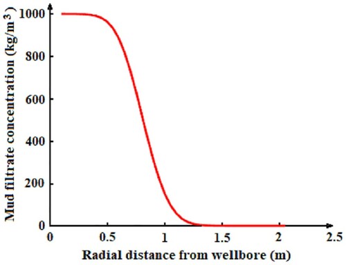
Figure 3. Mudcake growth: Dirichlet–Neumann boundary conditions, well no. 1.
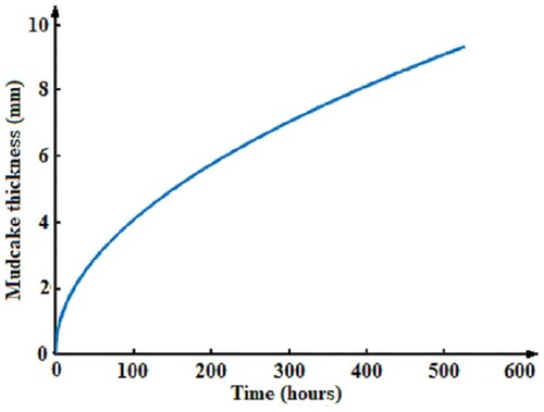
Figure 4. The optimal control (filtration rate) for Dirichlet–Neumann boundary conditions, well no 1: red dashed line – optimal control obtained with formulas (Equation3(3)
(3) ); blue line – optimal control obtained with formula (Equation135
(135)
(135) ).
![Figure 4. The optimal control (filtration rate) for Dirichlet–Neumann boundary conditions, well no 1: red dashed line – optimal control obtained with formulas (Equation3(3) u(t)=uMkcklnrerwkcklnrerw−ln(1−ξc(t)rw),(3) ); blue line – optimal control obtained with formula (Equation135(135) u∗(t)={u(0)−u∞tfort∈[0,t1)umfort∈[t1,t2)u∞(t−T)+u(T)fort∈[t2,T],(135) ).](/cms/asset/a43d26a9-08cd-4772-a8b7-928beb650df6/gipe_a_1914605_f0004_oc.jpg)
Figure 5. Mud filtrate dispersion values, well no 1: red dashed line – optimal control obtained with formulas (Equation3(3)
(3) ); blue line – optimal control obtained with formula (Equation135
(135)
(135) ).
![Figure 5. Mud filtrate dispersion values, well no 1: red dashed line – optimal control obtained with formulas (Equation3(3) u(t)=uMkcklnrerwkcklnrerw−ln(1−ξc(t)rw),(3) ); blue line – optimal control obtained with formula (Equation135(135) u∗(t)={u(0)−u∞tfort∈[0,t1)umfort∈[t1,t2)u∞(t−T)+u(T)fort∈[t2,T],(135) ).](/cms/asset/60d93c0f-70cf-4ca9-b31d-67906d9a439b/gipe_a_1914605_f0005_oc.jpg)
Figure 6. The optimal control (filtration rate) for Dirichlet–Neumann boundary conditions, well no 2: red dashed line – optimal control obtained with formulas (Equation3(3)
(3) ); blue line – optimal control obtained with formula (Equation135
(135)
(135) ).
![Figure 6. The optimal control (filtration rate) for Dirichlet–Neumann boundary conditions, well no 2: red dashed line – optimal control obtained with formulas (Equation3(3) u(t)=uMkcklnrerwkcklnrerw−ln(1−ξc(t)rw),(3) ); blue line – optimal control obtained with formula (Equation135(135) u∗(t)={u(0)−u∞tfort∈[0,t1)umfort∈[t1,t2)u∞(t−T)+u(T)fort∈[t2,T],(135) ).](/cms/asset/3b10876a-a06c-4c90-8d2a-161c9887d5b2/gipe_a_1914605_f0006_oc.jpg)
Figure 7. Mud filtrate dispersion values, well no 2: red dashed line – optimal control obtained with formulas (Equation3(3)
(3) ); blue line – optimal control obtained with formula (Equation135
(135)
(135) ).
![Figure 7. Mud filtrate dispersion values, well no 2: red dashed line – optimal control obtained with formulas (Equation3(3) u(t)=uMkcklnrerwkcklnrerw−ln(1−ξc(t)rw),(3) ); blue line – optimal control obtained with formula (Equation135(135) u∗(t)={u(0)−u∞tfort∈[0,t1)umfort∈[t1,t2)u∞(t−T)+u(T)fort∈[t2,T],(135) ).](/cms/asset/bd8d19a1-5824-4a84-90c0-0bc9a449ff2e/gipe_a_1914605_f0007_oc.jpg)
Figure 8. The optimal control (filtration rate) for Dirichlet–Neumann boundary conditions, well no 3: red dashed line – optimal control obtained with formulas (Equation3(3)
(3) ); blue line – optimal control obtained with formula (Equation135
(135)
(135) ).
![Figure 8. The optimal control (filtration rate) for Dirichlet–Neumann boundary conditions, well no 3: red dashed line – optimal control obtained with formulas (Equation3(3) u(t)=uMkcklnrerwkcklnrerw−ln(1−ξc(t)rw),(3) ); blue line – optimal control obtained with formula (Equation135(135) u∗(t)={u(0)−u∞tfort∈[0,t1)umfort∈[t1,t2)u∞(t−T)+u(T)fort∈[t2,T],(135) ).](/cms/asset/1f91a7ff-9d8b-4567-b2a4-cc77e22b9557/gipe_a_1914605_f0008_oc.jpg)
Figure 9. Mud filtrate dispersion values, well no 3: red dashed line – optimal control obtained with formulas (Equation3(3)
(3) ); blue line – optimal control obtained with formula (Equation135
(135)
(135) ).
![Figure 9. Mud filtrate dispersion values, well no 3: red dashed line – optimal control obtained with formulas (Equation3(3) u(t)=uMkcklnrerwkcklnrerw−ln(1−ξc(t)rw),(3) ); blue line – optimal control obtained with formula (Equation135(135) u∗(t)={u(0)−u∞tfort∈[0,t1)umfort∈[t1,t2)u∞(t−T)+u(T)fort∈[t2,T],(135) ).](/cms/asset/b2768da4-38fc-4bdf-8e71-06a6ac0b390b/gipe_a_1914605_f0009_oc.jpg)
Table 1. Well data, Windarto et al. [Citation1], wells 1 to 3, and Wu et al. [Citation18], well 4.
Table 2. Additional parameters, Windarto et al. [Citation1], wells 1 to 3, and Wu et al. [Citation18], well 4.
Table 3. The values of parameters
T and Pe.
Table 4. Comparison of mud filtrate dispersion values (formula (Equation160(160)
(160) )).
We find that condition (Equation134(134)
(134) ) is fulfilled only for the first three wells. The optimal control
obtained with formulas (Equation160
(160)
(160) ) (red line) and (Equation135
(135)
(135) ), respectively (blue line), are presented in Figures –.
5. Conclusion
In this paper, we have studied two inverse problems related to the invasion phenomenon. Our goal was to obtain as much information about the invasion rate as possible, if we do not have complete information about the values of all the physical quantities that appear in the mathematical model that describes the invasion phenomenon. We reduced these identification problems to two optimal control problems (minimization problems) in which the control is the invasion rate. We prove the existence of the solution of the state systems and the existence solution of minimization problems. We introduce the first-order variation systems, the dual systems and we prove that these systems have unique solutions. For each of the two problems we obtain the necessary condition of optimality by using the dual system. For the second problem we obtain a simple explicit form of control (filtration rate). We apply this explicit form of control in order to obtain the variation of the invasion rate using the data of three wells. Calculations can be made only if we know the values of Pe,
and
. Regarding the value
we can get information on the upper bound of this quantity (by using the formulas (Equation3
(3)
(3) ) and (Equation1
(1)
(1) )).
Acknowledgements
The author thanks the anonymous reviewers for the observations of an earlier form of this paper. The author acknowledges that the work of this paper was done during the doctoral internship at SCOSAAR, Romanian Academy.
Disclosure statement
No potential conflict of interest was reported by the author(s).
References
- Windarto, Gunawan AY, Sukarno P, et al. Modeling of formation damage due to mud filtrate invasion in a radial flow system. J Pet Sci Eng. 2012;100:99–105.
- Civan F. Reservoir formation damage. Fundamentals, assessment, and mitigation. Amsterdam: Elsevier; 2007.
- Donaldson EC, Chernoglazov V. Characterization of drilling mud fluid invasion. J Pet Sci Eng. 1987;1:3–13.
- Parn-anurak S, Engler TW. Modeling of fluid filtration and nearwellbore damage along a horizontal well. J Pet Sci Eng. 2005;46:149–160.
- Fertl WH. Log-derived evaluation of shaly classic reservoirs. J Pet Technol. 1987;39(2):175–187.
- Marinoschi G. Functional approach to nonlinear models of water flow in soils. Dordrecht: Springer; 2006.
- Marinoschi G, Favini A. Degenerate nonlinear diffusion equation. Berlin: Springer; 2012.
- Dautray R, Lions JL. Mathematical analysis and numerical methods for science and technology. Vol. 5. Berlin: Springer-Verlag; 1992.
- Aubin JP. Une théorème de compacité. C R Acad Sci Paris Série I. 1963;256:5042–5044.
- Lang S. Real analysis. London: Addison-Wesley Publishing Company; 1983.
- Colli P, Gilardi G, Marinoschi G. A boundary control problem for a possibly singular phase field system with dynamic boundary conditions. J Math Anal Appl. 2016;434:432–463.
- Oden JT, Kikuchy T. Theory of variational inequalities with applications to problems of flow through porous media. Int J Engng Sci. 1980;18:1173–1284.
- Barbu V. Mathematical methods in optimization of differential systems. Dordrecht: Kluwer Academic Publishers; 1994.
- Marinoschi G, Mininni RM, Romanelli S. An optimal control problem in coefficients for a strongly degenerate parabolic equation with interior degeneracy. J Optim Theory Appl. 2017;173:56–77.
- Fragnelli G, Marinoschi G, Mininni RR, et al. Identification of a diffusion coefficient in strongly degenerate parabolic equations with interior degeneracy. J Evol Equ. 2014;15(1):27–51.
- Evans LC. Partial differential equations. Providence (RI): American Mathematical Society; 2010.
- Boaca T, Malureanu I. Determination of oil reservoir permeability from resistivity measurement: a parabolic identification problem. J Pet Sci Eng. 2017;153:345–354.
- Wu J, Torres-Verdin C, Sempehrnoori K, et al. The influence of water-base mud properties and petrophysical parameters on mudcake growth, filtrate invasion, and formation pressure. Petrophysics. 2005;46(1):14–32.