Identification of airborne pollutant sources within a slot ventilated porous enclosure depending on backward model and downwind scheme

ABSTRACT

Identification of pollutant source, depending on the inverse computational fluid dynamics (CFD) methodology, within a slot-ventilated porous enclosure has been proposed in this paper. The whole fluid flow system is assumed to be two-dimensional, laminar and porous-saturated. As the inverse CFD modeling was ill-posed, a downwind scheme is employed to discretize the convection term to improve the accuracy and the corresponding time step range is derived to achieve numerical stability. Afterward, the downwind scheme simplifies the discretization process and its direct inversion algorithm. The effects of the Reynolds number ($2\times {10}^2\le Re\le 1\times {10}^4$), the Darcy number ($5\times {10}^{-5}\le Da\le 5\times {10}^{-3}$), the Schmidt number ($\text{0}\text{.1}\le Sc\le \text{2}$) and locations of pollutant source on the backward time CFD simulations are investigated, respectively. Results show that the temporal size/step is a critical factor of computational stability. In addition, the thickness of velocity or concentration boundary layer directly impacts the sensitivity of the inverse CFD simulation. The present research could aid in the safety of gas-supplying pipe network and relevant pollutant leakage accidents.

Highlights

• Identification of prior-unknown sources was proposed regarding gas-supplying network.

• Original transport equations were maintained to enhance the accuracy and generality.

• The downwind convection scheme was implemented to enhance backward CFD procedures.

• Diverse influencing factors were numerically tested to recover pollutant sources.

• The proposed new algorithm was validated thoroughly by experiments and benchmark solutions.

KEYWORDS:

• Enclosure convection
• inverse CFD modeling
• downwind schemes
• porous medium
• numerical stability

Nomenclature

D	=	mass diffusivity, m2/s
Da	=	Darcy number
H	=	dimensionless height of the enclosure
k	=	permeability, m2
l	=	length, m
p	=	fluid pressure, pa
P	=	dimensionless fluid pressure or position
Re	=	Reynolds number
Sh	=	Sherwood number
s	=	mass fraction
S	=	dimensionless mass fraction
Sc	=	Schmidt number
t	=	dimensionless time
t*	=	time, s
uj	=	velocity component in j-direction, m/s
Uj	=	dimensionless velocity component in j-direction
W	=	dimensionless width of the enclosure
xj	=	coordinate in j-direction, m
Xj	=	dimensionless coordinate in j-direction
$\mathrm{\Psi }$	=	streamfunction
T	=	dimensionless temperature
$\mathrm{\Gamma }$	=	effective diffusivity

Greek symbols

Δs	=	concentration scale
Ν	=	kinematics viscosity, m2/s
ρ	=	fluid density, kg/m3
$\varphi$	=	porosity

Subscripts

0, 1	=	reference value
cs	=	contaminant source
i, j	=	coordinate direction indices
in	=	inlet
max	=	maximum
min	=	minimum
port	=	inlet/outlet vent

1. Introduction

In case pollutants were frequently found in porous environments, such as chemical transport in packed-bed reactors, grain storage, food processing and storage and contaminant transport in ground water, the pollutant sources should be identified so that appropriate actions could be taken on time. Generally, the spatial distributions of airflow and pollutant concentrations in such enclosed porous environment could be measured by sensors. Using the spatial distributions of pollutant concentrations as initial conditions, one could solve reversely the pollutant transport equation to find the original source locations [1–4].

1.1. CFD: direct and inverse problems

Computational fluid dynamics (CFD) is a powerful tool for simulating the fluid flow and pollutant transport. To solve the distributions of pollutant concentration, one needs boundary conditions, initial conditions, physical properties and geometric characteristics of the porous environment, which were called as the direct CFD modeling or the cause–effect relationship. The literature concerning the convective flow in porous media is abundant. A rich variety of important analytical, numerical and experimental results have been published on this topic and they are important to understand better the convection inside porous enclosures [5–11]. Whereas, an inverse CFD modeling aims to find the causes, such as location and strength of the pollutant source, depending on the final effects, i.e. spatial distributions of airflow and pollutant concentrations.

The direct CFD modeling (forward-time simulation) is well-posed, as it satisfies the solution existence, uniqueness and stability [1]. However, an inverse CFD modeling could not be reproduced in experiments, due to the fact that the cause–effect relationship could not be physically reversed. For an inverse CFD modeling of pollutant transport in an enclosed porous environment, the solution physically exists when the flow field could be known as a prior. However, an inverse CFD solution may not be unique because different causes may lead to identical results. Inverse CFD solutions could become unique when assumptions of unknown casual characteristics were valid [2]. According to different causal characteristics, inverse CFD problems can be classified into the following four categories: boundary, retrospective, coefficient and geometric problems. The present case of identifying the unknown contaminant source location could be categorized into the retrospective one.

1.2. Instability of inverse problems and their three representative approaches

Computational instability, as stated by Alifanov [3], is the primary problem for the solution of an inverse problem, which directly causes the inverse CFD modeling ill-posed. Ill-posed inverse problems occurred in different fields, including heat transfer, groundwater transport and indoor contaminant transport; these inverse modeling solutions could be categorized into analytical, optimization, probabilistic and direct approaches. Each methodology has been illustrated well by Atmadja and Bagtzoglou [2] and Zhang and Chen [26]. The analytical approach requires analytical solution of the distributions of thermal and contaminant concentrations, then the causal characteristics are inversely solved. It has been applied to heat conduction problems [3,12] and groundwater contaminant transport [13,14]. However, analytical method is only suitable for simple problems so that the applications are very limited.

The optimization approach adopted direct modeling to obtain the effectual data based on all possible causal characteristics, such as distributions of contaminant concentrations. Then, a solution which is best-fitted with the corresponding measured data could be obtained through some optimization methods. At an early stage, this approach mainly focused on the identification of groundwater pollution sources by the linear optimization method [15], the maximum likelihood method [16] and the non-linear optimization method [17,18]. Because all of these optimization methods need to fully consider the possible causal characteristics, a large amount of direct modeling should be completed. Recently, the conjugate gradient method has been successfully applied to the inverse natural convection problem of estimating boundary heat fluxes [19,20].

The probabilistic approach uses probability to express a possible causal aspect. The pollutant source information is determined by maximizing or minimizing the probability objective function. Some representative researches can be tracked, such as the Bayesian probability model, integration of sensor network or adjoint probability method with fluid flow simulations [21–24]. The theory and implementation are complicated.

Direct approach was applied to solve inverse problems, through directly reversing the governing equations. The regularization technique [1] or the stabilization technique [28] has been implemented to improve the solution stability. For regularization technique, the solution is obtained by minimizing the objective function with a regularized term. As to stabilization technique, it introduces some stabilization terms into the reversed governing equations or solves some auxiliary equations to improve the solution stability. The quasi-reversibility (Q-R) method which belongs to direct approach is successfully applied to an indoor contaminant source identification [25–28] and reported that it costs less computational effort than the regularization technique and performs well, even if initial data were contained with some uncertainties [29,30].

1.3. Novel direct methodology and application for flows in porous medium

In the present work, direct approach will be adopted as it has less requirement of information about pollutant sources than the other inverse approaches. It also aims to propose a new direct method that is more simple and effective in this paper.

Fluid flow is essentially of directions, in other words, the state of any spatial point is dominated by its upstream one together with its passing time. Therefore, if time went reversely, the state of spatial point should be determined by the downstream one; although it was impossible in practice, temporal or spatial reverse in numerical calculation could be operated by the stabilization technique. As an evidence, establishment of the effect–cause relationship is the key issue and the discretization of convection term could be the most important breakthrough point. Specifically, the upwind scheme of convection term is physically reasonable and stable for time forward calculation, whereas the downwind scheme of convection term could be appropriate for backward calculation. If our primary guess really worked, backward simulation methodology would be more simple and effective than the Q-R method.

2. Physical model and mathematical formulations

In this research, ideal scenarios, including room air flows without radiation, rectangular enclosures, measurements without errors, to name just a few, will be assumed to allow dispersal of airborne pollutants and transport within room airflow structures, and pollutant’s concentrations in some regions could be effectively ‘measured’ or ‘detected’. Undoubtedly, measurements of sensors could influence the inverse solutions, whatever the solution accuracy and reliability. However, for this primary research, novel methodology and procedure will be proposed, and these could be exercised and validated by present ideal situations, such as the followings.

It is assumed that the third dimension of the enclosure is large enough such that the fluid and mass transports are of two dimensions. The porous matrix is assumed to be uniform and in local compositional equilibrium with the saturating fluid. Physical properties are considered to be constant. The flow is assumed to be laminar, incompressible and with no thermal or solutal buoyancy. Viscous dissipation and porous medium inertia are intentionally avoided in the present work, and density of the saturated fluid mixture is assumed to be uniform over all the enclosure.

With the above-mentioned assumptions, the physically bounded domain under present investigation is a two-dimensional fluid-saturated Darcy–Brinkman porous enclosure which is attached with the bottom supplying vent and top exhaust port of same size $l_{\text{port}}$, respectively, on the left and right sides while other boundaries are impermeable, as indicated in Figure 1. Cartesian coordinates (x, y), with the corresponding velocity components (u, v), are also indicated herein. The rectangular enclosure is of width W and height H, and the aspect ratio of the entire calculation domain is maintained at H/W=1/2.

Figure 1. Flow configuration and coordinate system.

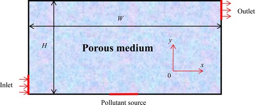
The governing equations based on the above assumptions are the Reynolds-averaged equations for mass continuity, momentum and species conservation. At time t = 0, the strip contaminant sources of constant strength begin to release pollutants inside the cavity. The dimensionless time-averaged equations for mass, momentum and species conservations are as follows: (1) $\begin{array}{rl}\frac{\mathrm{\partial }{U}_j}{\mathrm{\partial }{X}_j}& =0j=1,2\end{array}$(1) (2) $\begin{array}{rl}\frac{\mathrm{\partial }{U}_i{U}_j}{\mathrm{\partial }{X}_j}& =-\frac{\mathrm{\partial }P}{\mathrm{\partial }{X}_i}+\frac{1}{Re}\frac{\mathrm{\partial }}{\mathrm{\partial }{X}_j}\left(\frac{\mathrm{\partial }{U}_i}{\mathrm{\partial }{X}_j}\right)-\frac{U_i}{Re\cdot Da}i,j=1,2\end{array}$(2) (3) $\begin{array}{rl}\frac{\mathrm{\partial }S}{\mathrm{\partial }t}+\frac{\mathrm{\partial }S{U}_j}{\mathrm{\partial }{X}_j}& =\frac{1}{Sc\cdot Re}\frac{\mathrm{\partial }}{\mathrm{\partial }{X}_j}\left(\frac{\mathrm{\partial }S}{\mathrm{\partial }{X}_j}\right)j=1,2\end{array}$(3)

In Equation (3), the dimensionless transport equation of pollutants could be divided into three terms, namely unsteady term, convection term and diffusion term. Following dimensionless variables were applied, (4a) $\begin{array}{rl}{X}_j& =x_j/H,U_j=u_j/U_0,t=t^{\ast }/\left(H/U_0\right)\end{array}$(4a) (4b) $\begin{array}{rl}P& =p/\left(\rho U_0^2\varphi \right),S=(s-s_0)/\mathrm{\Delta }s\end{array}$(4b) (5) $\begin{array}{rl}{U}_0& =u_{in},\mathrm{\Delta }s=s_1-s_0\end{array}$(5) where $H$, $U_0$, $H/U_0$ and $\mathrm{\Delta }s$ have been used as the characteristic scales for length, velocity, time and concentration, respectively. Correspondingly, dimensionless governing parameters, namely the Reynolds number Re, the Darcy number Da and the Schmidt number Sc could be defined, respectively, as follows: (6) $Re=\frac{u_{in}H}{\nu }{\varphi }^{-1},Da=k/H^2,Sc=\frac{\nu }{D}\varphi$(6) The symbols $\nu$, D, k and $\varphi$ denote, respectively, the kinematics viscosity of the fluid, the molecular diffusivity of the combined fluid plus solid porous matrix medium, the permeability of the porous medium and the porosity of porous medium, respectively. It should be noted here that the Reynolds number and Schmidt number have been naturally modified by porosity.

The boundary conditions sketched in Figure 1 are illustrated as follows: (7a) $\begin{array}{rl}\text{Inlet}\text{and}\text{outlet}(l_{\text{port}}& =0.1H):U=1,V=0,\frac{\mathrm{\partial }\text{S}}{\mathrm{\partial }\text{X}}\text{ = 0}\end{array}$(7a) (7b) $\begin{array}{rl}\text{Contaminant}\text{source}(l_{\text{cs}}& =0.1H):U=0,V=0,S=1\end{array}$(7b) (7c) $\begin{array}{rl}\text{Vertical walls}:U& =0,V\text{ = 0,}\frac{\mathrm{\partial }\text{S}}{\mathrm{\partial }\text{X}}\text{ = 0}\end{array}$(7c) (7d) $\begin{array}{rl}\text{Horizontal walls}:U& =0,V=0,\frac{\mathrm{\partial }\text{S}}{\mathrm{\partial }\text{Y}}\text{ = 0}\end{array}$(7d)

Aforementioned boundary conditions indicate that no-slip conditions are imposed on the walls and global mass conservation is applied to simplify the numerical procedure for the velocity profile of outlet [31]. As the velocity profile at the inlet and outlet is constant and the two velocity values before and after are equal in the iterative calculation process, the boundary condition of zero gradient is adopted in the pressure correction equation.

Upon steady fluid flow has been achieved, mass transfer potential across the system can be evaluated directly by the overall mass transfer rate along the pollutant source, (8) $Sh=\frac{1}{l_{cs}}{\int }_{l_{cs}}{-\frac{\mathrm{\partial }S}{\mathrm{\partial }Y}|}_{Y=0}dX$(8)

Stream function and streamlines are routinely the best way to visualize the convective fluid flow. The dimensionless streamfunction Ψ is defined such that, (9) $\frac{\mathrm{\partial }\mathrm{\Psi }}{\mathrm{\partial }Y}=U,-\frac{\mathrm{\partial }\mathrm{\Psi }}{\mathrm{\partial }X}=V$(9)

3. Direct CFD numerical procedure and code validation

The finite volume method (FVM) was applied to discretize the above-governing Equations (1)–(3) on a staggered grid system [32]. In the course of discretization, the second-order upwind scheme and central difference scheme are, respectively, implemented for the convection and diffusion terms. The Semi-Implicit Method for Pressure Linked Equations (SIMPLE) algorithm was chosen to numerically solve the governing differential equations in their primitive forms [20,27]. The pressure correction equation was obtained from the continuity equation to enforce local mass balance along the boundaries [28,31]. To obtain better convergence properties, unsteady terms in species Equation (3) were implicitly treated and hence approximated by the backward differencing scheme, as explained in Section 4. For each time step, an iterative process is adopted, and the discretized equations were solved via combining the successive over-relaxation (SOR) iterations [23].

So as to obtain grid independence results, several categories of uniform grid numbers, namely $81\times 41$, $121\times 61$, $201\times 101$ and $241\times 121$ were tried. These numerical experiments demonstrated that the final uniform grid size of $201\times 101$ was adequate to describe the fluid flow and mass diffusion process correctly. Further increase in the number of grid points produced essentially similar results. Table 1 illustrated the grid independence of the predictions for $Re=2.0\times {10}^3$ and $Da=2.5\times {10}^{-3}$. It can be seen that the solution for mass transfer rate $Sh$ was almost independent on the mesh size when the grid numbers were no $<201\times 101$ (within 2%).

Table 1. Grid independence validation: Sh number for different grid resolution.

Grid sizes	41×81	61×121	101×201	121×241
Sh	17.63	24.30	26.26	26.73

To verify the accuracy of the present numerical investigation, the present procedure was validated by performing simulations for the flow between parallel plates with the classical partially filled porous media. As shown in Figure 2, upper and lower walls were attached with porous media layers of the same thickness, and the middle layer was a pure fluid zone. The length of the two parallel plates was theoretically infinite, so the flow at the right exit is fully developed. The flow chart of direct CFD procedure simulation algorithm could be observed in Figure 3. Depending on the axial velocity of the fully developed flow presented in the above model, the calculated results of this program are shown in Figure 4. Comparing with the data in the literature [33], one could observe that the results calculated from present program were in good agreements with those from the reference [33]. Moreover, Figure 5 clearly shows that the computed horizontal velocity and temperature through the vertical centerline are in excellent agreement with those of Khanafer and Chamkha [34] in the porous medium lid-driven cavity. Overall, favorable comparisons have set up confidence in the accuracy of the numerical results of the present work.

Figure 2. A schematic diagram of the flow through two parallel-plate channel partially filled with two porous substrates.

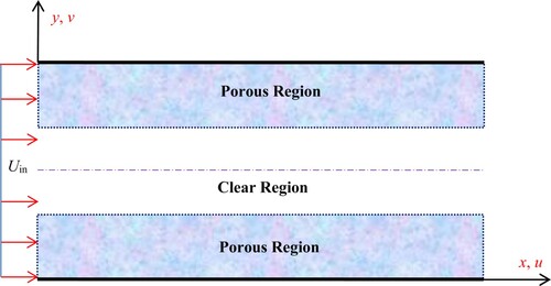
Figure 3. Flow chart of direct CFD procedure simulation algorithm.

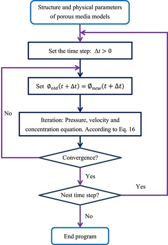
Figure 4. A comparison of the present work fully developed axial velocity with the solution given by Alkam et al. [33] for $Da=1\times {10}^{-4}$.

Figure 5. Comparison of the velocity and temperature profiles between the present prediction and Khanafer and Chamkha [34].

4. Theory of inverse CFD modeling and its procedure

The identification of pollutant sources actually represents the solution of an inverse problem. History of pollutant dispersion has been recorded by the ‘measurements’ inside the ventilated porous enclosure, in which the places of emission will be identified by the backward simulation methodology. Most attempts at quantifying contaminant transport rely on solving the species equation. To reconstruct the spatial spread of airborne pollutants, one needs to solve the governing equation backward in time, such like the following equation: (10) $\frac{\mathrm{\partial }S}{\mathrm{\partial }t}=-\frac{\mathrm{\partial }S{U}_j}{\mathrm{\partial }{X}_j}+\frac{\mathrm{\partial }}{\mathrm{\partial }{X}_j}\left(\mathrm{\Gamma }\frac{\mathrm{\partial }S}{\mathrm{\partial }{X}_j}\right)j=1,2$(10)

where $\mathrm{\Gamma }$ is the effective diffusivity and it is equivalent to $1/\left(Sc\cdot Re\right)$.

For two-dimensional, structured and uniform grid systems, Equation (10) can be discretized into the following format, $\begin{array}{rl}{S}_P\left(t+\mathrm{\Delta }t\right)& =\frac{\frac{\left[\right[U_w,0\left]\right]}{\mathrm{\Delta }X}+\frac{\mathrm{\Gamma }}{\mathrm{\Delta }{X}^2}}{A}\cdot S_W\left(t+\mathrm{\Delta }t\right)+\frac{\frac{\left[\right[-U_e,0\left]\right]}{\mathrm{\Delta }X}+\frac{\mathrm{\Gamma }}{\mathrm{\Delta }{X}^2}}{A}\cdot S_E\left(t+\mathrm{\Delta }t\right)\\ & +\frac{\frac{\left[\right[V_s,0\left]\right]}{\mathrm{\Delta }Y}+\frac{\mathrm{\Gamma }}{\mathrm{\Delta }{Y}^2}}{A}\cdot S_S\left(t+\mathrm{\Delta }t\right)\\ & +\frac{\frac{\left[\right[-V_n,0\left]\right]}{\mathrm{\Delta }Y}+\frac{\mathrm{\Gamma }}{\mathrm{\Delta }{Y}^2}}{A}\cdot S_N\left(t+\mathrm{\Delta }t\right)+\frac{\frac{1}{\mathrm{\Delta }t}}{A}\cdot S_P\left(t\right)\end{array}$ (11) $A=\frac{1}{\mathrm{\Delta }t}+\frac{\left[\right[U_e,0\left]\right]+\left[\right[-U_w,0\left]\right]}{\mathrm{\Delta }X}+\frac{\left[\right[V_n,0\left]\right]+\left[\right[-V_s,0\left]\right]}{\mathrm{\Delta }Y}+2\mathrm{\Gamma }\left(\frac{1}{\mathrm{\Delta }{X}^2}+\frac{1}{\mathrm{\Delta }{Y}^2}\right)$(11) Here, the discretized Equation (11) has employed the first-order upwind scheme and central difference scheme which are, respectively, implemented for the convection term and diffusion term. There is no problem for forward simulation in aspect of computational stability [35].

Most situations of interest here will be such that the value of a dependent variable at a grid point is influenced by the values at neighboring grid points only through the processes of convection and diffusion. Then, it follows that an increase in the value at one grid point should, with other conditions remaining unchanged, leads to an increase (and not a decrease) in the value at the neighboring grid point. However, if the temporal step is negative ($\mathrm{\Delta }t<0$, i.e. backward simulation), the sign of the coefficient A of $S_P\left(t+\mathrm{\Delta }t\right)$ is <1, while the coefficients of neighbor nodes (W, E, S and N) will be negative. According to the positive coefficient rule [27], the coefficient of the central node P should have the same sign as the coefficient of the adjacent nodes in the discrete process, and if this rule was violated, a physically unrealistic solution will be got. That is, only those formulations that guarantee positive coefficients under all circumstances will be accepted. Also, this is the root cause of numerical instability for solving inverse problem directly, namely the ill-posed characteristics. Of course, a large temporal step size can relax the instability, in other words, a small absolute value of $1/\mathrm{\Delta }t$ makes the coefficient of $S_P\left(t+\mathrm{\Delta }t\right)$ positive. However, it results in a malpractice that very small coefficient of $S_P\left(t\right)$ will not have a substantial impact on inverse solutions.

Currently, the Q-R method is universally applied to solve such inverse problems by adding a fourth-order stability term into the original governing equation to suppress the numerical divergence in backward time modeling. Usually, this method solves the diffusion equation with the reversed time by replacing the original diffusion operator $\frac{\mathrm{\partial }}{\mathrm{\partial }t}-{\mathrm{\nabla }}^2$ with the Q-R operator $\frac{\mathrm{\partial }}{\mathrm{\partial }t}-{\mathrm{\nabla }}^2-ϵ{\mathrm{\nabla }}^4$, where $ϵ$ is a small positive stabilization constant and ${\mathrm{\nabla }}^2$ stands for the Laplace operator.

As to forward simulation, the concentration on some interface depends on upstream nodes, which is the so-called upwind scheme, while for backward simulation it should rely on the downstream nodes, which can be named downwind scheme. Take the interface e as an example, (12) $S_e=\{\begin{array}{l}{S}_E,U_e>0\\ S_P,U_e<0\end{array}$(12) The same process was followed for other interfaces (w, n and s) and the final discretized Equation (13) is obtained for backward simulation, $\begin{array}{rl}{S}_P\left(t+\mathrm{\Delta }t\right)& =\frac{\frac{-\left[\right[-U_w,0\left]\right]}{\mathrm{\Delta }X}+\frac{\mathrm{\Gamma }}{\mathrm{\Delta }{X}^2}}{A^{\ast }}\cdot S_W\left(t+\mathrm{\Delta }t\right)+\frac{\frac{-\left[\right[U_e,0\left]\right]}{\mathrm{\Delta }X}+\frac{\mathrm{\Gamma }}{\mathrm{\Delta }{X}^2}}{A^{\ast }}\cdot S_E\left(t+\mathrm{\Delta }t\right)\\ & +\frac{\frac{-\left[\right[-V_s,0\left]\right]}{\mathrm{\Delta }Y}+\frac{\mathrm{\Gamma }}{\mathrm{\Delta }{Y}^2}}{A^{\ast }}\cdot S_S\left(t+\mathrm{\Delta }t\right)\\ & +\frac{\frac{-\left[\right[V_n,0\left]\right]}{\mathrm{\Delta }Y}+\frac{\mathrm{\Gamma }}{\mathrm{\Delta }{Y}^2}}{A^{\ast }}\cdot S_N\left(t+\mathrm{\Delta }t\right)+\frac{\frac{1}{\mathrm{\Delta }t}}{A^{\ast }}\cdot S_P\left(t\right)\end{array}$ (13) $A^{\ast }=\frac{1}{\mathrm{\Delta }t}-\frac{\left[\right[-U_e,0\left]\right]+\left[\right[U_w,0\left]\right]}{\mathrm{\Delta }X}-\frac{\left[\right[-V_n,0\left]\right]+\left[\right[V_s,0\left]\right]}{\mathrm{\Delta }Y}+2\mathrm{\Gamma }\left(\frac{1}{\mathrm{\Delta }{X}^2}+\frac{1}{\mathrm{\Delta }{Y}^2}\right)$(13) To achieve the computational stability, we can make all the coefficients negative as far as possible. Additionally, the coefficient of $S_P\left(t+\mathrm{\Delta }t\right)$ should be smaller than −1, that is to say, (14) $\frac{1}{\mathrm{\Delta }t}-\frac{\left[\right[-U_e,0\left]\right]+\left[\right[U_w,0\left]\right]}{\mathrm{\Delta }X}-\frac{\left[\right[-V_n,0\left]\right]+\left[\right[V_s,0\left]\right]}{\mathrm{\Delta }Y}+2\mathrm{\Gamma }\left(\frac{1}{\mathrm{\Delta }{X}^2}+\frac{1}{\mathrm{\Delta }{Y}^2}\right)<-1$(14) Then, the inequality (13) is equivalent to the next one, (15) $\frac{1}{\mathrm{\Delta }t}<-1-2\mathrm{\Gamma }\left(\frac{1}{\mathrm{\Delta }{X}^2}+\frac{1}{\mathrm{\Delta }{Y}^2}\right)+\left(\frac{\left[\right[-U_e,0\left]\right]+\left[\right[U_w,0\left]\right]}{\mathrm{\Delta }X}+\frac{\left[\right[-V_n,0\left]\right]+\left[\right[V_s,0\left]\right]}{\mathrm{\Delta }Y}\right)$(15) For the right part of inequality (15), because the term, $\left(\frac{\left[\right[-U_e,0\left]\right]+\left[\right[U_w,0\left]\right]}{\mathrm{\Delta }X}+\frac{\left[\right[-V_n,0\left]\right]+\left[\right[V_s,0\left]\right]}{\mathrm{\Delta }Y}\right)$, is always positive, inequality (16) is consequently valid, (16) $\mathrm{\Delta }t>{\left(-1-2\mathrm{\Gamma }\left(\frac{1}{\mathrm{\Delta }{X}^2}+\frac{1}{\mathrm{\Delta }{Y}^2}\right)\right)}^{-1}$(16) Thus, if the downwind scheme works in backward simulation, the condition of inequality (16) should be satisfied.

At the same time, if the coefficients of neighbor nodes are all negative, then a set of inequalities (17) is required, (17) $\{\begin{array}{l}\left[\right[-U_w,0\left]\right]\mathrm{\Delta }X>\mathrm{\Gamma }\\ \left[\right[U_e,0\left]\right]\mathrm{\Delta }X>\mathrm{\Gamma }\\ \left[\right[-V_s,0\left]\right]\mathrm{\Delta }Y>\mathrm{\Gamma }\\ \left[\right[V_n,0\left]\right]\mathrm{\Delta }Y>\mathrm{\Gamma }\end{array}$(17) Actually, it implies that not all nodes can meet the above set of inequalities especially those close to boundaries or are in any other regions of low velocity, because the convective intensity may be so weak that diffusion effect is predominant.

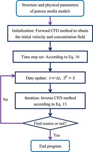
According to the inverse modeling theory in this section, initial distributions of airflow and contaminant concentration are not the only requirements for a successful inverse CFD modeling. The present inverse CFD modeling also requires boundary conditions, physical properties and geometric characteristics. For the slot-ventilated porous enclosure of this interest, physical properties and geometric characteristics were assumed as constants in the present inverse CFD modeling. Thus, boundary conditions become the key factors in determining the source locations. During the forward CFD modeling, some portions of pollutants might have been exited out of the enclosure through outlets, whereas the extracted pollutants should be ‘traced back’ into the domain as the boundary conditions for the inverse or backward CFD simulations. Additionally, other boundaries as Dirichlet conditions should be treated as Neumann ones. In other words, the mass flow rate is zero for unknown boundary information of pollutants. The solution process of Equation (13), therefore, is similar to the forward algorithm, unlike Q-R or any other methodologies [14]. The last issue that needs to be prepared in the starting procedure is to determine an appropriate time step. The flow chat of an inverse time simulation algorithm has been illustrated in Figure 6.

Figure 6. Flow chart of inverse time simulation algorithm.

Figure 7 describes the flow field and pollutant concentration field in the displacement ventilation enclosure without porous media. The Q-R method and present proposed method have been, respectively, applied to the identification of implicit pollutant sources. The results of the backward CFD modeling can be seen in Figure 8. Observing from source locations identified by both methodologies, results from present one could be better than those from the Q-R one; particularly, the present procedure costed fewer calculation cycles with identical temporal step size.

Figure 7. Streamlines (left) and pollutant concentration fields (right) with Re=1.0×10³, Sc=0.6 at t=100.

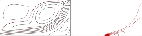
Figure 8. The inverse results of pollutant source location, Q-R (left) and new study (right).

5. Results and discussion

The direct CFD methodology was first adopted to obtain the spatial distributions of fluid flow and species spread, and some of its episode could be treated as an initial data for backward CFD simulations. In practice, initial field data could only be measured by sensors for inverse CFD modeling. Clearly scrutinizing the procedure of this inverse CFD, it is appropriate to apply the direct CFD model here to ‘produce’ initial data.

The problem under investigation is governed by three dimensionless parameters, i.e. Re, Da and Sc. Moreover, pollutant source locations, numbers and diffusion intensities are all important factors affecting the spread of pollutants. The computed streamlines and iso-concentrations are plotted in the following figures and the intervals of these isopleths are determined by the relation of $\mathrm{\Delta }S=\left(S_{max}-S_{min}\right)/16$.

5.1. Effect of temporal step size on backward simulation

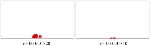
The airborne pollutant source was originally assumed to be centrally located on the floor. The limitation of temporal step should be first confirmed. The flow field and spatial concentration distributions are produced under the conditions of Re=2×10³, Sc=0.8 and Da=2.5×10⁻³, as shown in Figure 9.

Figure 9. Streamlines (left) and pollutant concentration fields (right) with Re=2×10³, Sc=0.8, Da=2.5×10⁻³ at t=150

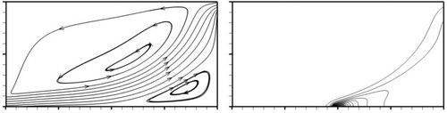
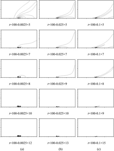
According to the formulation of (16), temporal step $\mathrm{\Delta }t$ should be higher than −0.0588. Backward CFD simulations have been performed depending on three different temporal step sizes which, respectively, includes $\mathrm{\Delta }t=-0.025$, $\mathrm{\Delta }t=-0.05$ and $\mathrm{\Delta }t=-0.1$, and numerical results confirm that former two temporal steps were appropriate with the backward time simulation, as shown in Figure 10. It can be seen that the pollutant source location has been identified successfully in the first two cases as shown in Figure 10(a, b). Perturbation first occurs near the pollutant source and then the residuals of pollutant concentration asymptotically converge to the original position of pollutant source. Furthermore, a larger temporal step size leads to a faster identification, but the history of pollutant dispersion in space is not presented in detail. Unsurprisingly, it is of failure in the last case that the result is totally wrong as shown in Figure 10(c) (t=150–0.1×7). For the case of $\mathrm{\Delta }t=-0.1$, a very small under relaxation factor was actually required to run the inverse solution procedure due to a strong instability, though the results have been proved to be worthless. Hence, the limitation of temporal step size, i.e. the inequality (16), is reasonable and essential, and most of the difficulty in backward time simulation is then avoided.

Figure 10. Effect of temporal step size on backward simulation with Re=2×10³, Sc=0.8 and Da=2.5×10⁻³, (a) Δt=−0.025, (b) Δt=−0.05, and (c) Δt=−0.1

5.2. Effect of Re and Da on backward simulation

The Reynolds number (i.e. supplying velocity herein in present model) certainly affects the fluid flow and pollutant dispersion, and also influences such inverse CFD solution process. Regarding backward CFD simulations, the Reynolds number not only determines the effective temporal step size as described in Section 5.1, but also has a serious impact on the thickness of velocity boundary layer which confirms the usability of the set of formulations (17).

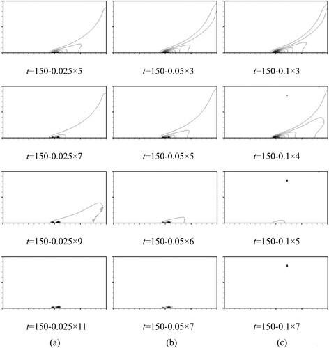
As long as the temporal steps could be feasible, different ones almost bring identical identification results under a specific situation with a single source on the floor, just as presented in Figure 10(a, b). Therefore, it is appropriate to apply inconsistent temporal step sizes to research the effect of Re on backward CFD simulations. Three values of the Reynolds number include 2×10², 2×10³ and 1×10⁴, whereas the Darcy number and Schmidt number are maintained at 5×10⁻⁴ and 0.8, respectively. Accordingly, temporal steps of $\mathrm{\Delta }t=-0.0025$, $\mathrm{\Delta }t=-0.025$ and $\mathrm{\Delta }t=-0.1$ are separately selected. Flow fields and pollutant concentration distributions under different Reynolds numbers are plotted in Figure 10. With Re increasing from 2×10² to 1×10⁴, the number of eddies increases from 0 to 2, and the contaminated area gradually shrinks, which means that the dispersion effect has been gradually inhibited.

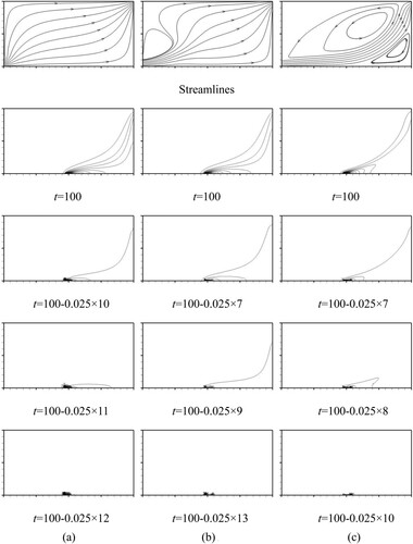
Results of backward CFD simulation are presented in Figure 11. After several tests of some temporal steps, the pollutant source location could be successfully identified. In addition, the spatial evolution of pollutant dispersion was inversely computed, though the temporal evolution certainly was of some deviation from the direct process, it could still be a benefit for the rapid inverse identification of contaminant source location. Obviously illustrated in Figure 12, for backward CFD simulation, a lower Reynolds number directly causes a more massive perturbation or distortion above the pollutant source from the final time points of these three cases. This is due to the fact that the lower Reynolds number with a thicker velocity boundary layer does not adequately satisfy the formulation of (17). In other words, the downwind scheme of convection term is more applicable for the flow of high Reynolds number or even the flow of diffusion term neglected. Of course, it also works for the flow that diffusion is predominant though the accuracy is lost in some level.

Figure 11. Streamlines (left) and pollutant concentration fields (right) with Sc=0.8, Da=5×10⁻⁴ at t=100, (a) Re=2×10², (b) Re=2×10³, and (c) Re=1×10⁴

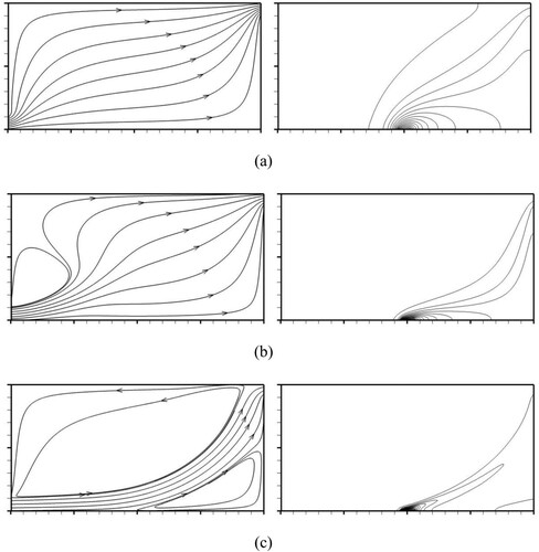
Figure 12. Effect of Re on backward simulation with Sc=0.8 and Da=5×10⁻⁴, (a) Re=2×10², (b) Re=2×10³, and (c) Re=1×10⁴

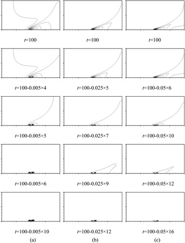
The Darcy number, i.e. the permeability of porous matrix, has an important influence on airflow fields, but it does not directly affect concentration distributions. Da only impacts the serviceability of inequalities (17) by altering the velocity field. Observing from Figure 13, a more massive perturbation above the pollutant source appeared under a lower Darcy number, which is similar to the effect of Re. It will not be given a redundant explanation in this article.

Figure 13 Streamlines and backward simulations with Re=2×10³, Sc=0.8, (a) Da=5×10⁻⁵, (b) Da=5×10⁻⁴, and (c) Da=5×10⁻³.

5.3. Effects of Sc on backward simulation

The Schmidt number, as described in the governing Equations (1)–(3), is just a factor that affects the concentration fields without considering solutal buoyancy. Though Sc also determines the practicable range of temporal step according to inequality (16), it has been illustrated in Section 5.2 that all of the feasible time steps almost lead to the same identification result. Thus, it can be tested if the concentration distribution itself affects the inverse solution by changing the value of Sc. Three values are, respectively, assigned for Sc which are 0.1, 0.8 and 2.0, while Re=2×10³ and Da=2.5×10⁻³, and the temporal steps are −0.005, −0.025 and −0.05 in order.

The corresponding flow structure has been shown in Figure 9 and the inversely computed concentration fields are presented in Figure 14. With an increasing Sc, the diffusibleness of pollutants decrease so that the contaminanted area is reduced at t=100. Essentially, a higher Sc (smaller effective diffusivity $\mathrm{\Gamma }$) produces a thinner concentration boundary layer such that more grid nodes should be clustered toward the wall vicinity to meet the formulation of (17). Therefore, the region of distortion is reduced for a higher Sc, which represents a higher accurary of pollutant source identification.

Figure 14. Effect of Sc on backward simulation with Re=2×10³ and Da=2.5×10⁻³, (a) Sc=0.1, (b) Sc=0.8, and (c) Sc=2.0.

5.4. Effects of locations of pollutant sources on backward simulation

The single pollutant source centrally positioned on the floor has been inversely identified, under different dimensionless parameters in previous sections. Then, the inverse model will be tested for double pollutant sources in this section. Admittedly, different positions of pollutant sources will affect the inverse identification. Here are two arrangements of pollutant sources: case 1, where two sources of same size l_cs are both located on the floor, and case 2, where two sources are both within the porous enclosure. Three dimensionless governing parameters are maintained as follows: Re=2×10³, Da=2.5×10⁻³ and Sc=0.8.

For case 1, the two pollutant sources are symmetrically placed along the vertical center line with a distance W/2. The initial concentration field and inverse solutions are presented in Figure 15(a). One can see that the two pollutant sources are both identified successfully, but the amplitudes of perturbation above these two pollutant source locations are quite different as a result of unequal thicknesses of velocity boundary layers. The identified pollutant source (t=100–0.025×9) near inlet port is only characterized by a single line, which may be a trouble because it can be easily drowned out by strong noise from the other source.

Figure 15. Effect of pollutant sources on backward simulation with Re=2×10³, Da=2.5×10⁻³, Sc=0.8 and Δt=−0.025.

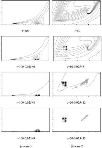
As expected, what was worried did happen in case 2 as shown in Figure 15(b). The two square pollutant source zones with side length l_cs are symmetrically located on the horizontal central line along the vertical central line, with a distance of W/2. The source on the left is quite accurately identified for the three of four vertexes inversely computed out. However, the source on the right is obliterated due to its weaker distortion which is caused by immersing in the flow with much stronger convection, even though the perturbation of non-source zone is stronger than it. Because the real location and number of pollutant sources are unknown beforehand in practice, the inversion results in Figure 15 must be of some mistake.

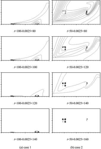
To solve the problem, the part of inverse solution data were drowned as mentioned previous, there is no other ways but to employ a smaller temporal step size (such as Δt=−0.0025) to solve the two cases again for reducing the polarization of perturbation amplitude, on account of that the inequalities (17) are changeless for all nodes in a specific situation. Observing from Figure 16, the positions of pollutant sources are both correctly identified in case 1 and case 2, and the obstacle mentioned before is dexterously removed. Though the pollutant source zone on the right is not depicted vividly, it is enough to approximately fix its position. Therefore, it is conducive to generate a more reliable identification result by spending more time (i.e. using a smaller temporal step size) on the inverse procedure.

Figure 16. Effect of pollutant sources on backward simulation with Re=2×10³, Da=2.5×10⁻³, Sc=0.8 and Δt=−0.0025

6. Conclusions

Forward and backward CFD simulations of air flow inside the porous region have been conducted in the present work. Within the slot-ventilated porous enclosure, after the steady air flow structures have been established, one or two pollutant sources are assumed to emit airborne pollutants. A downwind scheme is proposed to discretize the convection term when the primitive pollutant dispersion equation was directly solved with reverse time steps. The releasing history of airborne pollutants has been recovered by our self-developed codes, concerning the effects of temporal step size, supplying velocity, permeability of porous medium, pollutant diffusivity and pollutant source position and its numbers.

An inverse CFD modeling with a downwind scheme for convection terms could identify pollutant source locations. The proposed new numerical scheme has simplified the discretization process and facilitated the direct inversion algorithm. Temporal step has become a critical factor for computational stability. A smaller time step size generates a more detailed spatial evolution history, but more importantly, it produces a more credible identification result as the pollutant source location and numbers were unknown as prior.

Thicknesses of momentum and species concentration boundary layers directly impact the sensitivity of backward CFD simulations. A higher Reynolds number or Darcy number could reduce the distortion region around the pollutant source due to a thinner velocity boundary layer forms. Similarly, a higher Schmidt number could result in a thinner concentration boundary layer, which also reduces the region of distortion. Moreover, the Reynolds number and Schmidt number determine the suitable range of temporal step for inverse CFD modeling.

In addition, the coupled heat and mass transport in porous medium ventilation enclosure is worth studying. Physical problems with the presence of heat transport are quite common, so it is necessary to incorporate thermal factors into systematic researches in subsequent steps.

Further researches should be conducted for some actual situations, for example, more sparse grids (less observation points), noise data of measurements, incomplete data of concentration fields especially at the outlet, and test of higher order downwind scheme, turbulence, to name just a few.

Disclosure statement

No potential conflict of interest was reported by the author(s).

Additional information

Funding

This research was financially supported by the Provincial Key R&D Program of Hunan ([grant number 2022SK2084], Hunan University of Technology), the Youth Science and Technology Innovation Leader of Hunan Province ([grant number 2020RC4032], Hunan University of Technology), the Wuhan Application Foundation and Cutting-edge Research Plan ([grant number 2020010601012206], the Wuhan Municipal Council), the Shandong Provincial Natural Science Foundation [grant number ZR2018MEE035] and the Natural Science Foundation of China (NSFC) ([grant number 51778504], [grant number U1867221], Wuhan University).

References

- Tikhnovo AN, Arsenin VY. Solutions of ill-posed problems. Washington: Halsted press; 1977.
- Atmadja J, Bagtzoglou AC. State of the art report on mathematical methods for groundwater pollution source identification. Environ Forensics. 2001;2(2):205–214. DOI:10.1006/enfo.2001.0055
- Alifanov OM. Inverse heat transfer problems. New York: Springer-Verlag; 1994.
- Sun NZ. Inverse problems in groundwater modeling. Boston: Kluwer Academic; 1994.
- Selimefendigil F, Ztop HF. Effects of local curvature and magnetic field on forced convection in a layered partly porous channel with area expansion. Int J Mech Sci. 2020;179:105696. DOI:10.1016/j.ijmecsci.2020.105696
- Selimefendigil F, Ztop HF. Combined effects of double rotating cones and magnetic field on the mixed convection of nanofluid in a porous 3D U-bend. Int Commun Heat Mass Transfer. 2020;116:104703. DOI:10.1016/j.icheatmasstransfer.2020.104703
- Selimefendigil F, Ztop HF. Magnetohydrodynamics forced convection of nanofluid in multi-layered U-shaped vented cavity with a porous region considering wall corrugation effects. Int Commun Heat Mass Transfer. 2020;113:104551. DOI:10.1016/j.icheatmasstransfer.2020.104551
- Selimefendigil F, Ztop HF. Thermal management and modeling of forced convection and Entropy Generation in a vented cavity by Simultaneous Use of a curved porous layer and magnetic field. Entropy . 2021;23(2):152. DOI:10.3390/e23020152
- Hussai S, Ahmed SE, Akbar T. Entropy generation analysis in MHD mixed convection of hybrid nanofluid in an open cavity with a horizontal channel containing an adiabatic obstacle. Int J Heat Mass Transfer. 2017;114:1054–1066. DOI:10.1016/j.ijheatmasstransfer
- Ahmed SE. Mixed convection in thermally anisotropic non-Darcy porous medium in double lid-driven cavity using Bejan's heatlines. Alexandria Eng J. 2016;55(1):299–309. DOI:10.1016/j.aej.2015.07.016
- Hussai S, Ahmed SE, Saleem F. Impact of periodic magnetic field on Entropy Generation and mixed convection. J Thermophys Heat Transfer. 2018;32(4):999–1012. DOI:10.2514/1.T5430
- Frankel JI. Residual-Minimization least-squares method for inverse heat conduction. Comput Math Appl. 1996;32(1):117–130. DOI:10.1016/0898-1221(96)00130-7
- Ala NK, Domenico PA. Inverse analytical techniques applied to coincident contaminant distributions at otis air force base, massachusetts. Ground Water. 1992;30(2):212–218. DOI:10.1111/j.1745-6584.1992.tb01793.x
- Alapati S, Kabala ZJ. Recovering the release history of a groundwater contaminant using a non-linear least-squares method. Hydrol Process. 2000;14(6):1003–1016. DOI:10.1002/(SICI)1099-1085(20000430)14:6<1003::AID-HYP981>3.0.CO;2-W
- Gorelick SM, Evans BE, Remson I. Identifying sources of groundwater pollution: an optimization approach. Water Resour Res. 1983;19(7):779–790. DOI:10.1029/WR019i003p00779
- Wagner BJ. Simultaneous parameter estimation and contaminant source characterization for coupled groundwater flow and contaminant transport modelling. J Hydrol. 1992;135(1-4):275–303. DOI:10.1016/0022-1694(92)90092-A
- Mahar PS, Datta B. Identification of pollution sources in transient groundwater systems. Water Res Man. 2000;14(3):209–227. DOI:10.1023/A:1026527901213
- Mahar PS, Datta B. Optimal identification of ground-water pollution sources and parameter estimation. J Water Res Pl. 2001;127(1):20–29.
- Prud’homme M, Nguyen TH. Solution of inverse free convection problems by conjugate gradient method: effects of Rayleigh number. Int J Heat Mass Transfer. 2001;44(11):2011–2027. DOI:10.1016/S0017-9310(00)00266-0
- Zhao FY, Liu D, Tang GF. Inverse determination of boundary heat fluxes in a porous enclosure dynamically coupled with thermal transport. Chem Eng Sci. 2009;64(7):1390–1403. DOI:10.1016/j.ces.2008.12.005
- Sohn MD, Reynolds P, Singh N, et al. Rapidly locating and characterizing pollutant releases in buildings. J Air Waste Manage Assoc. 2002;52(12):1422–1432. DOI:10.1080/10473289.2002.10470869
- Arvelo J, Brandt A, Roger RP. An enhancement multi-zone model and its application to optimum placement of CBW sensors. ASHRAE Trans. 2002;108(2):818–825.
- Liu D, Zhao FY, Yang H, et al. Probability adjoint identification of airborne pollutant sources depending on one sensor in a ventilated enclosure with conjugate heat and species transports. Int J Heat Mass Transfer. 2016;102:919–933. DOI:10.1016/j.ijheatmasstransfer.2016.06.023
- Liu X, Zhai Z. Location identification for indoor instantaneous point contaminant source by probability-based inverse computational fluid dynamics modeling. Indoor Air. 2008;18(1):2–11. DOI:10.1111/j.1600-0668.2007.00499.x
- Liu D, Zhao FY, Wang HQ. History recovery and source identification of multiple gaseous contaminants releasing with thermal effects in an indoor environment. Int J Heat Mass Transfer. 2012;55(1):422–435. DOI:10.1016/j.ijheatmasstransfer.2011.09.041
- Zhang TF, Chen Q. Identification of contaminant sources in enclosed environments by inverse CFD modeling. Indoor Air. 2007;17(3):167–177. DOI:10.1111/j.1600-0668.2006.00452.x
- Liu D, Zhao FY, Wang HQ, et al. History source identification of airborne pollutant dispersions in a slot ventilated building enclosure. Int J Therm Sci. 2013;64:81–92. DOI:10.1016/j.ijthermalsci.2012.08.005
- Lattes R, Lions JL. The method of quasi-reversibility, applications to partial differential equations. New York: Elsevier; 1969.
- Skaggs TH, Kabala ZJ. Recovering the history of a groundwater contaminant plume: method of quasi-reversibility. Water Resour Res. 1995;31(2):2669–2673. DOI:10.1029/95WR02383
- Bagtzogolou AC, Atmadja J. Marching-jury backward beam equation and quasi-reversibility methods for hydrologic inversion: application to contaminant plume spatial distribution recovery. Water Resour Res. 2003;39(2):1011–1014. DOI:10.1029/2001WR001021
- Zhao FY, Liu D, Tang L. Direct and inverse mixed convections in an enclosure with ventilation ports. Int J Heat Mass Transfer. 2009;52(19):4400–4412. DOI:10.1016/j.ijheatmasstransfer.2009.03.017
- Zhao FY, Liu D, Tang GF. Natural convection in a porous enclosure with a partial heating and salting element. Int J Therm Sci. 2008;47(5):569–583. DOI:10.1016/j.ijthermalsci.2007.04.006
- Alkam MK, Al-Nimr MA, Hamdan MO. On forced convection in channels partially filled with porous substrates. Heat Mass Transf. 2002;38(4-5):337–342. DOI:10.1007/s002310000177
- Khanafer KM, Chamkha AJ. Mixed convection flow in a lid-driven enclosure filled with a fluid-saturated porous medium. Int J Heat Mass Transfer. 1999;42(13):2465–2481. DOI:10.1016/S0017-9310(98)00227-0
- Patankar SV. Numerical heat transfer and fluid flow. Washington: Hemisphere Publishing Co.; 1980.