Recovery of thermal load parameters by means of the Monte Carlo method with fixed and meshless random walks

ABSTRACT

The paper is focused on the numerical analysis of the two-point inverse stationary heat flow problem, namely the identification of the thermal load. Determination of selected parameters is possible on the basis of temperature measurements, done at specified few locations. This problem may be modelled as the optimization problem, standard numerical analysis of which requires multiple solutions of boundary value problems. However, the novel solution approach, proposed here, is based on the well-known concept of the Monte Carlo method with an appropriate random walk technique. It yields explicit stochastic relations combining computed temperatures and all load parameters. Such relations may be directly applied in most standard optimization algorithms, replacing time-consuming solutions of systems of algebraic equations. Moreover, one may construct the semi-analytical approach, in which the unknown load parameters are obtained explicitly, allowing for the elimination of sensitiveness to initial solutions or requirements for admissible load intervals. The paper is illustrated with results of several benchmark problems with simulated measurement data and various numbers of unknown load parameters. The results comparison, between standard element-free methods with selected optimization algorithms as well as the proposed Monte Carlo solution approach is presented and is especially focused on CPU times.

KEYWORDS:

• Inverse problem
• heat flow problem
• finite difference method
• meshless methods
• Monte Carlo method
• random walk
• optimization problem

MATHS:

• 80A23

1. Introduction

Problems of civil engineering and mechanics may be classified as either forward or inverse ones. In case of forward problems, their parameters including geometry, material, load, are known, and therefore, the answer of a structure (displacements, eigen frequencies, stress, strain, temperature, heat flux) may be obtained in an unambiguous manner. In most cases, the mathematical model of forward problems constitutes the well-posed, linear or non-linear, initial-boundary problem. It may be solved by means of analytical (rarely) or numerical approaches, of both deterministic and stochastic natures. Deterministic (hard-computing) methods are based upon the domain discretization (mesh of nodes and/or elements) and unknown function approximation, which leads to the system of algebraic equations. For instance, Finite Element Method (FEM) [1], meshless methods [2,3], including standard [4] or meshless Finite Difference Method (FDM or MFDM) [5–7] as well as Boundary Element Method (BEM) [8] may be mentioned here. On the other hand, stochastic (soft-computing) methods may take solution randomness as well as uncertainties of parameters into account. On the contrary to deterministic approaches with fixed parameters' values, their random selection (e.g.from the admissible interval with assigned fuzziness) lead to the entire family of solutions out of which the optimal one has to be selected. This family of solutions may be parameterized in many different manners, depending on the applied method. Stochastic approaches may include Genetic and Evolutionary Algorithms [9,10], Monte Carlo methods [11], artificial neural networks [12] as well as fuzzy sets [13].

Whenever at least one of the above mentioned problem parameters is unknown, one deals with the inverse problem, more dificult in practical analysis and usually ill-posed, namely the solution existence, its uniqueness and stability are questionable, and strongly depend on the type and the number of additional data as well as assumptions of heuristic and experimental types [14].

The inverse problems may be classified as

• topology optimization problems [15–17], in which an unknown geometry has to be determined on the basis of additional additional criteria and hypotheses (e.g. the minimal mass of a structure or its maximal capacity),

• material identification problems [18–20], in which material parameters of designed or existing structure are either unknown or uncertain and have to be determined or examined on the basis of measurements of selected data,

• load identification problems [21–23], in which selected load parameters are unknown.

It is worth mentioning that both material and load identification problems belong to the wide SHM (Structural Health Monitoring [24]) branch, in which the lifetime duration and conditions of safe exploitation of an existing structure are frequently estimated on the basis of measurement data and appropriate inverse analysis. Selection of a proper number of sensors and their optimal location are one of the most important SHM issues [23,25,26]. However, a lack of commercial software, dedicated to an engineering, practical analysis of inverse problems, is a serious disadvantage in this field.

This research is focused on the numerical analysis of inverse heat conduction problems, which is an important aspect in various engineering fiels, like conduction, hydrology, transportation and diffusion in natural materials. It is assumed that selected load parameters (boundary temperature and/or boundary heat flux and/or heat source function) are unknown and have to be determined on the basis of few temperature measurements, performed at specified locations.

The solution approach as well as model order reduction techniques, applied to inverse heat problems, strongly depend on the type of additional data. The simplest and rather not realistic cases assume the existence of a continuous solution, partially given on the boundary or inside the domain. Therefore, the original problem may be transformed into the auxiliary problem, which is solved by means of traditional computational tools, mentioned earlier [27–30], which is followed by the inverse transformation. Consideration of noisy data requires additional restoration algorithms [31,32]. More general approaches are based upon the non-linear constrained optimization problem that is formulated and solved [33,34], incorporating aforementioned deterministic [35,36] as well as stochastic solution approaches [23,37]. Regardless of optimization algorithms (e.g. genetic algorithms [10,18,38], numerous variants of Gauss–Newton method [39], steepest descent methods), its numerical treatment requires multiple numerical solutions of auxiliary boundary value problems, for various values of unknown load parameters. Therefore, the appropriate numerical model of the heat flow problem has to be established, usually coupled with the optimization algorithm itself (e.g. method of fundamental solutions based upon old concept of Green's function [22,28,40,41], Singular Value Decomposition [42], Tikhonov regularization technique [36,43], fractional derivatives [44], including combinations with FEM [45], BEM [46] and meshless methods [20,28,30,47], as frequently reported in literature). Eventually, ill-conditioning of the original inverse problem is reduced by appropriate regularization techniques [35,48].

In this research, the stationary 1D heat flow problem is considered. Though it may not seem to be significantly challenging, the optimization problem dimensionality (aka the number of decision variables) should be taken into account. The standard FDM (on regular meshes), as well as the meshless FDM (MFDM, on arbitrarily irregular clouds of nodes with no mesh structure imposed), are effectively applied. The justification of such selection is based upon following arguments, namely the simplicity of the resulting algebraic FD model (since the local formulation of the heat transfer problem may be applied, integration and assembling are omitted), flexibility of the cloud of nodes, which may be adapted to the measurement locations without any difficulties, as well as the straightforward relationship of FD methods with Monte Carlo method and a random walk technique, developed here. However, both FD methods determine the temperature at all nodes of the mesh / cloud, independently of the number of measurement points, which is usually much smaller than the number of degrees of freedom of the numerical model (aka nodal temperature values). Therefore, the entire procedure is rather computationally demanding and time-consuming. A remedy would be an approach that allows to estimate the temperature only at those nodes which coincide with measurement points, without involving determination of temperature at other locations.

The Monte Carlo (MC) method [49,50] with a random walk technique offers such possibility. The concept of MC is based upon the series of random problem-oriented trials, and estimation of the solution using a ratio between the number of success trials and the number of all trails (providing it is large enough). Among its numerous applications in deterministic and probabilistic problems of functional mathematics and algebra, the stochastic estimation of the solution of differential equations at selected point(s) of the domain [11,51] is considered here. In case of optimization and inverse problems, the MC is usually related to the random sampling procedure [52–54], definition of a probability distribution in the model space [55], or noise filtering [56], even when combined with FD methods [57].

In this research, a novel application of MC to inverse problems is proposed. As the MC solution approach point-wise delivers an explicit linear relation of stochastic type between thermal load parameters and measured temperatures, it may be applied twofold, namely

1. as the replacement of the multiple solution of time-consuming systems of equations, arising from the application of standard numerical methods (FEM, standard or meshless FDM, BEM) and selected optimization algorithms; this variant does not remove drawbacks of later ones, however it may significantly decrease computational time; or

2. as the separate optimization method, which is based upon semi-analytical differentiation of the objective function and single solution of small, linear system of equations; this variant allows for removal of all drawbacks of standard optimization algorithms (searching through solution space, sensitivity to initial solution, divergent iterative procedure, requirement for admissible load intervals), not mentioning of superior speed-up factors.

Both variants are presented and examined in this research, for the first time ever. Regardless of variant's selection, the application of MC to forward and inverse boundary value problems requires construction of random walks, namely the randomly generated path (net of connections) leading from the point of interest and the problem boundary, where the solution is known. Statistics of all points visited along the path is taken into account. In case of load identification problems, such operation is performed only once for the entire solution process. For simple problem domains with rectangular meshes of points, the fixed random walk may be constructed, in which both moves directions and step sizes are a-priori pre-defined [11]. The MC with fixed random walk corresponds to the standard FD model of the original problem. However, in case the boundary value problem has more general form (mixed boundary conditions, complex geometry requiring irregular meshes/clouds of nodes, heterogeneous material functions), random walks of semi-floating (including meshless random walks) or full-floating type have to be constructed, in which moves directions and/or step sizes are not pre-defined and depend on the local points neighbourhood. The meshless random walk corresponds to and uses several principles of the meshless FD framework, for instance, nodes classification criteria [4–6,58] and the Moving Weighted Least Approximation (MWLS [4,59,60]) technique. The preliminaries of MC with meshless random walk and prototype Matlab code for forward problems have been presented in [51,61], whereas its application to various elliptic problems of mechanics may be found in [62].

Especially, the potential power of the second Monte Carlo variant, listed above, should be noted. The engineering, original or existing open-source software, based upon this approach, may effectively use the a-priori generated meshes on which random walks may be constructed (the first solution step). Afterwards, unknown load parameters are determined by means a small system of linear equations, which use all a-priori known material and load parameters (if any) as well as nodal indication numbers (the second solution step). The entire procedure may be automated and implemented without any difficulties. Potential users can refer to the included Matlab software.

The paper is organized in the following manner. Section 2 introduces three milestones of each inverse, identification problem, namely the formulation of a forward problem, characteristics of experimental data as well as the general optimization procedure. Section 3 recalls fundamentals of standard and meshless FD methods, whereas Section 4 presents Monte Carlo method with fixed (based upon standard FDM) and meshless (based upon meshless FDM) random walks. The selected optimization algorithms, including the novel, direct Monte Carlo optimization method, are briefly discussed in Section 5. Section 6 (with attached Matlab code) shows results of numerous benchmark examples with simulated measurement data and varying degrees of complexity as well as selected extensions of the proposed approach towards more complex heat conduction problems. Eventually, the paper concludes with an indication of possible directions for future work.

1.1. Notations

• T – temperature,

• λ – conductivity coefficient,

• ρ – mass density,

• c – specific heat capacity,

• α – Fourier coefficient,

• q – heat flux,

• $T_a$, $T_b$ – boundary temperatures,

• $q_a$, $q_b$ – boundary heat fluxes,

• f – heat source function,

• $\mathbf{T}$ – temperature parameters (degrees of freedom),

• $\mathbf{f}$ – heat source parameters (degrees of freedom),

• n – number of nodes for discretization of T function,

• $\mathbf{x}$ – coordinates of nodes for discretization of T function,

• $m_f$ – number of nodes for discretization of f function,

• $\overline{\mathbf{x}}$, ${\mathbf{x}}_f$ – coordinates of constriction points/nodes for discretization of f function,

• $\mathbf{\Phi }$ – basis functions for approximation of f function,

• $m_t$ – number of temperature measurements,

• $\hat{\mathbf{x}}$ – coordinates of temperature measurement points,

• $\hat{\mathbf{T}}$ – temperature measurements,

• $\mathrm{\Delta }T$ – measurement tolerance (error),

• ${\mathbf{M}}_f$ – coefficient matrix for mapping of f values between $\mathbf{x}$ and ${\mathbf{x}}_f$,

• F – objective function,

• $\mathbf{P}$ – set of decision variables (thermal parameters),

• ${\mathbf{P}}^{\left(\mathrm{o}\mathrm{p}\mathrm{t}\right)}$ – optimal thermal parameters,

• ${\mathbf{P}}^{\left(\mathrm{l}\mathrm{o}\mathrm{w}\mathrm{e}\mathrm{r}\right)}$ – lower error bounds of thermal parameters,

• ${\mathbf{P}}^{\left(\mathrm{u}\mathrm{p}\mathrm{p}\mathrm{e}\mathrm{r}\right)}$ – upper error bounds of thermal parameters,

• $\mathbf{K}$ – conductivity matrix,

• $\mathbf{F}$ – thermal load vector,

• h – mesh modulus,

• $\mathbf{M}$ – coefficient matrix resulting from the MWLS approximation,

• N – total number of random walks,

• $p_i$, $p_{i,k}$ – probabilities of the next move,

• $N_{i,j}$, $N_{(i,j),(k,l)}$ – nodal indication numbers.

1.2. Glossary

• inverse heat conduction problem – heat conduction problem in which both temperature and thermal load may be unknown,

• objective function – mean squared error between computed temperatures at measurement points and measured temperatures, related to measurement tolerance,

• decision variables – set of unknown thermal parameters,

• difference star – configuration of nodes used for construction of the local approximation of the unknown function,

• difference operator – linear combination of known/unknown function values used as a replacement of value of differential operator at point,

• standard finite difference method (FDM) – a method of numerical analysis of boundary value problems which uses regular meshes and standard difference operators built on stars with the minimal required number of nodes,

• moving weighted least squares (MWLS) approximation – technique of local approximation used in meshless methods which provides the set of local function derivatives using Taylor series expansion and weighted mean squared error,

• meshless finite difference method (MFDM) – a meshless method which may deal with arbitrarily irregular clouds of nodes and which uses MWLS approximation for generation of difference operators,

• random walk – a randomly constructed path leading from the particular point of the domain to its boundary,

• fixed random walk – a type of random walk in which both step size and move directions are fixed,

• meshless random walk – a type of floating random walk in which both step size and move directions may change from node to node,

• indication numbers – numbers of nodal visits/hits counted along the path of each random walk,

• Monte Carlo method/simulation – a method that allows for an estimation of unknown solution on the basis of randomly generated trails,

• direct Monte Carlo optimization method – a method that allows for semi-analytical solution of the optimization problem.

2. Problem formulation

The following stationary thermal model with the anisotropic material is considered: find such a temperature $C^2$ (2nd-order continuously differentiable) function, $T:(\mathrm{\Re }\times {\mathrm{\Re }}^{m_p})\to \mathrm{\Re }$ and $T=T(x,\mathbf{P}){[}^{\mathrm{o}}\mathrm{C}]$, which satisfies the following two-point boundary value problem (1) $\{\begin{array}{l}T(a,\mathbf{P})=T_a,x=a,\\ -{\displaystyle \frac{\mathrm{d}\lambda }{\mathrm{d}x}}{\displaystyle \frac{\mathrm{\partial }T}{\mathrm{\partial }x}}-\lambda \left(x\right){\displaystyle \frac{{\mathrm{\partial }}^{2}T}{\mathrm{\partial }{x}^2}}=f(x,\mathbf{f}),x\in (a,b)\\ \lambda \left(b\right){\displaystyle \frac{\mathrm{\partial }T}{\mathrm{\partial }x}}(b,\mathbf{P})=q_b,x=b.\end{array}$(1) with the vector $\mathbf{P}$, consisting of $m_p$ thermal load parameters (2) $\mathbf{P}=[T_a,q_b,{\mathbf{f}}^{\mathrm{\top }}]=[T_a,q_b,f_1,f_2,\dots ,f_{m_f}]$(2) Here, $a\left[\mathrm{m}\right]$ and $b\left[\mathrm{m}\right]$ are the left and right ends of the domain interval, respectively; $f=f(x,\mathbf{f}):(\mathrm{\Re }\times {\mathrm{\Re }}^{m_f})\to \mathrm{\Re }$ is the intensity $C^0$ function of heat generation inside the domain (internal heat source function), $\lambda =\lambda \left(x\right)\left[{\mathrm{J}/(\mathrm{m}\mathrm{s}}^{\mathrm{o}}\mathrm{C}\right)]$ is the known heat conductivity positive material $C^1$ function ($\lambda \left(x\right)>0,\mathrm{\forall }x\in [a,b]$), whereas $T_a{[}^{\mathrm{o}}\mathrm{C}]$ and $q_b\left[{\mathrm{J}/(\mathrm{m}}^2\mathrm{s}\right)]$ are boundary temperature and heat flux, respectively.

In case of the forward problem, $T_a$, $q_b$ are known scalar numbers, $f=f\left(x\right)\left[{\mathrm{J}/(\mathrm{m}}^3\mathrm{s}\right)]$ is a known scalar function, whereas $T=T\left(x\right)$ is the primary unknown function. Moreover, the problem (1(1) $\{\begin{array}{l}T(a,\mathbf{P})=T_a,x=a,\\ -{\displaystyle \frac{\mathrm{d}\lambda }{\mathrm{d}x}}{\displaystyle \frac{\mathrm{\partial }T}{\mathrm{\partial }x}}-\lambda \left(x\right){\displaystyle \frac{{\mathrm{\partial }}^{2}T}{\mathrm{\partial }{x}^2}}=f(x,\mathbf{f}),x\in (a,b)\\ \lambda \left(b\right){\displaystyle \frac{\mathrm{\partial }T}{\mathrm{\partial }x}}(b,\mathbf{P})=q_b,x=b.\end{array}$(1) ) is well-posed then. However, in case of the inverse problem, either entire or selected load parameters may be unknown. Those may include numbers $T_a$ and $q_b$ as well as the formula for the heat source function f. Providing f is unknown, it has to be explicitly approximated, for instance, on the basis of its $m_f$ control (construction) points $({\overline{x}}_j,f_j)$, regularly spaced in the problem domain. Coordinates ${\overline{x}}_j$ are fixed, whereas degrees of freedom $f_j$ remain undetermined. Consequently, the heat source function f may be expressed in the following manner (3) $f(x,\mathbf{f})=\sum _{j=1}^{m_f}{\mathrm{\Phi }}_j\left(x\right)f_j=\mathbf{\Phi }\left(x\right)\mathbf{f}$(3) in which $\mathbf{\Phi }\left(x\right)=\left\{{\mathrm{\Phi }}_j\right(x\left)\right\}$ is the assumed $[1\times m_f]$ vector of dimensionless basis functions and $\mathbf{f}=\left\{f_j\right\}$ is the $[m_f\times 1]$ vector of heat source' degrees of freedom (with the same physical units as the function f, namely $\left[{\mathrm{J}/(\mathrm{m}}^3\mathrm{s}\right)]$). In all following formulas, physical units, introduced here, are omitted for the sake of simpler notations.

The unknown load vector $\mathbf{P}$ may include, in most general case, $m_p=m_f+2$ unknown load parameters. It has to be stressed that the set of control points $({\overline{x}}_j,f_j)$ should not be confused with a discretization mesh of a physical dimension $x\in [a,b]$, which is introduced in Section 3. Therefore, the mathematical model (1(1) $\{\begin{array}{l}T(a,\mathbf{P})=T_a,x=a,\\ -{\displaystyle \frac{\mathrm{d}\lambda }{\mathrm{d}x}}{\displaystyle \frac{\mathrm{\partial }T}{\mathrm{\partial }x}}-\lambda \left(x\right){\displaystyle \frac{{\mathrm{\partial }}^{2}T}{\mathrm{\partial }{x}^2}}=f(x,\mathbf{f}),x\in (a,b)\\ \lambda \left(b\right){\displaystyle \frac{\mathrm{\partial }T}{\mathrm{\partial }x}}(b,\mathbf{P})=q_b,x=b.\end{array}$(1) ) remains continuous, in spite of approximation schemes, applied for an unknown heat source function at this early stage of research.

In order to avoid imminent ill-possedness of the inverse problem (1(1) $\{\begin{array}{l}T(a,\mathbf{P})=T_a,x=a,\\ -{\displaystyle \frac{\mathrm{d}\lambda }{\mathrm{d}x}}{\displaystyle \frac{\mathrm{\partial }T}{\mathrm{\partial }x}}-\lambda \left(x\right){\displaystyle \frac{{\mathrm{\partial }}^{2}T}{\mathrm{\partial }{x}^2}}=f(x,\mathbf{f}),x\in (a,b)\\ \lambda \left(b\right){\displaystyle \frac{\mathrm{\partial }T}{\mathrm{\partial }x}}(b,\mathbf{P})=q_b,x=b.\end{array}$(1) ), components of (2(2) $\mathbf{P}=[T_a,q_b,{\mathbf{f}}^{\mathrm{\top }}]=[T_a,q_b,f_1,f_2,\dots ,f_{m_f}]$(2) ) have to be determined on the basis of additional information, namely temperature measurements ${\hat{T}}_i$ at $m_t$ isolated internal points ${\hat{x}}_i$ (4) ${\hat{T}}_i\pm \mathrm{\Delta }{T}_i,i=1,2,\dots ,m_t$(4) with assigned measurement tolerances $\mathrm{\Delta }{T}_i$ each. The inverse problem may be ill-posed, providing the number of measurement points is insufficient ($m_t<m_p$) or measurement points are distributed in an inappropriate manner. In that case, small parameters modification may result in enormous differences in $\mathbf{P}$.

The mathematical model of (1(1) $\{\begin{array}{l}T(a,\mathbf{P})=T_a,x=a,\\ -{\displaystyle \frac{\mathrm{d}\lambda }{\mathrm{d}x}}{\displaystyle \frac{\mathrm{\partial }T}{\mathrm{\partial }x}}-\lambda \left(x\right){\displaystyle \frac{{\mathrm{\partial }}^{2}T}{\mathrm{\partial }{x}^2}}=f(x,\mathbf{f}),x\in (a,b)\\ \lambda \left(b\right){\displaystyle \frac{\mathrm{\partial }T}{\mathrm{\partial }x}}(b,\mathbf{P})=q_b,x=b.\end{array}$(1) ), taking into account (4(4) ${\hat{T}}_i\pm \mathrm{\Delta }{T}_i,i=1,2,\dots ,m_t$(4) ), may be formulated in terms of the non-linear optimization problem, namely (5) ${\mathbf{P}}^{\left(\mathrm{o}\mathrm{p}\mathrm{t}\right)}=\underset{\left(\mathbf{P}\right)}{\mathrm{a}\mathrm{r}\mathrm{g}\mathrm{m}\mathrm{i}\mathrm{n}}F\left(\mathbf{P}\right),F\left(\mathbf{P}\right)=\sqrt{\frac{1}{m_t}\sum _{i=1}^{m_t}{\left({\displaystyle \frac{T({\hat{x}}_i,\mathbf{P})-{\hat{T}}_i}{\mathrm{\Delta }{T}_i}}\right)}^2}$(5) where F is the objective function, whereas components of $\mathbf{P}$ are decision variables. The objective function is selected in a most general manner and may be considered as the mean squared error between the computed $T({\hat{x}}_i,\mathbf{P})$ and measured ${\hat{T}}_i$ temperatures (4(4) ${\hat{T}}_i\pm \mathrm{\Delta }{T}_i,i=1,2,\dots ,m_t$(4) ) that involves the analytical or numerical solution of (1(1) $\{\begin{array}{l}T(a,\mathbf{P})=T_a,x=a,\\ -{\displaystyle \frac{\mathrm{d}\lambda }{\mathrm{d}x}}{\displaystyle \frac{\mathrm{\partial }T}{\mathrm{\partial }x}}-\lambda \left(x\right){\displaystyle \frac{{\mathrm{\partial }}^{2}T}{\mathrm{\partial }{x}^2}}=f(x,\mathbf{f}),x\in (a,b)\\ \lambda \left(b\right){\displaystyle \frac{\mathrm{\partial }T}{\mathrm{\partial }x}}(b,\mathbf{P})=q_b,x=b.\end{array}$(1) ) at measurement points ${\hat{x}}_i$ for temporarily fixed load parameters $\mathbf{P}$. Moreover, such selection of F allows for consideration of an arbitrary number and locations of measurements as well as it does not require any a-priori knowledge concerning the unknown thermal load parameters. Finally, F involves measurement tolerance whereas its dimensionless definition allows for combining of measurements of various types (for instance, additional heat flux measurements, a case not considered here).

Moreover, $m_t$ local inequality constraints result from (4(4) ${\hat{T}}_i\pm \mathrm{\Delta }{T}_i,i=1,2,\dots ,m_t$(4) ) and may be expressed as (6) $|T({\hat{x}}_i,\mathbf{P})-{\hat{T}}_i|<\mathrm{\Delta }{T}_i,i=1,2,\dots ,m_t$(6) Although the optimization problem is formulated in the unbounded domain, the following numerical analysis as well as practical aspects require the definition of the admissible space ${\mathbf{P}}^{\left(adm\right)}$, such that (7) $\mathbf{P}\in {\mathbf{P}}^{\left(adm\right)}=[{\mathbf{P}}^{(min)},{\mathbf{P}}^{(max)}]$(7) Each component of $\mathbf{P}$ may have its own limits, namely (8) $T_a\in [T_a^{(min)},T_a^{(max)}],q_b\in [q_b^{(min)},q_b^{(max)}],f_j\in [f^{(min)},f^{(max)}],j=1,\dots ,m_f$(8) The necessary condition for the existence of the global extreme of (5(5) ${\mathbf{P}}^{\left(\mathrm{o}\mathrm{p}\mathrm{t}\right)}=\underset{\left(\mathbf{P}\right)}{\mathrm{a}\mathrm{r}\mathrm{g}\mathrm{m}\mathrm{i}\mathrm{n}}F\left(\mathbf{P}\right),F\left(\mathbf{P}\right)=\sqrt{\frac{1}{m_t}\sum _{i=1}^{m_t}{\left({\displaystyle \frac{T({\hat{x}}_i,\mathbf{P})-{\hat{T}}_i}{\mathrm{\Delta }{T}_i}}\right)}^2}$(5) ) leads to the following system of $m_p$ equations with $m_p$ unknowns (9) ${\mathbf{\nabla }}_{\mathbf{P}}F\left(\mathbf{P}\right)=\mathbf{0}$(9) After substitution of F from (5(5) ${\mathbf{P}}^{\left(\mathrm{o}\mathrm{p}\mathrm{t}\right)}=\underset{\left(\mathbf{P}\right)}{\mathrm{a}\mathrm{r}\mathrm{g}\mathrm{m}\mathrm{i}\mathrm{n}}F\left(\mathbf{P}\right),F\left(\mathbf{P}\right)=\sqrt{\frac{1}{m_t}\sum _{i=1}^{m_t}{\left({\displaystyle \frac{T({\hat{x}}_i,\mathbf{P})-{\hat{T}}_i}{\mathrm{\Delta }{T}_i}}\right)}^2}$(5) ) to (9(9) ${\mathbf{\nabla }}_{\mathbf{P}}F\left(\mathbf{P}\right)=\mathbf{0}$(9) ), the following formula is obtained (10) ${\mathbf{\nabla }}_{\mathbf{P}}F\left(\mathbf{P}\right)=2\sum _{i=1}^{m_t}{\displaystyle \frac{T({\hat{\mathbf{x}}}_i,\mathbf{P})-{\hat{T}}_i}{\mathrm{\Delta }{T}_i^2}}{\mathbf{\nabla }}_{\mathbf{P}}T({\hat{\mathbf{x}}}_i,\mathbf{P})$(10) in which ${\mathbf{\nabla }}_{\mathbf{P}}T$ is the $[m_p\times 1]$ temperature gradient with respect to $\mathbf{P}$, given by (11) ${\mathbf{\nabla }}_{\mathbf{P}}T(x,\mathbf{P})=\{\frac{\mathrm{\partial }T}{\mathrm{\partial }{P}_i}\left(x\right),i=1,2,\dots ,m_p\}$(11) For selected optimization methods as well as for the examination of the necessary condition of the minimum existence of F at $\mathbf{P}$, a matrix of second derivatives (Hessian) of F with respect to $\mathbf{P}$, denoted as ${\mathbf{H}}_{\mathbf{P}}F$ (12) $\begin{array}{rl}{\mathbf{H}}_{\mathbf{P}}F\left(\mathbf{P}\right)& ={\mathbf{\nabla }}_{\mathbf{P}}\otimes \left({\mathbf{\nabla }}_{\mathbf{P}}F\left(\mathbf{P}\right)\right)\\ & =2\sum _{i=1}^{m_t}{\displaystyle \frac{{\mathbf{\nabla }}_{\mathbf{P}}T({\hat{\mathbf{x}}}_i,\mathbf{P}){\mathbf{\nabla }}_{\mathbf{P}}^{\mathrm{\top }}T({\hat{\mathbf{x}}}_i,\mathbf{P})+(T({\hat{\mathbf{x}}}_i,\mathbf{P})-{\hat{T}}_i){\mathbf{H}}_{\mathbf{P}}T({\hat{x}}_i,\mathbf{P})}{\mathrm{\Delta }{T}_i^2}}\end{array}$(12) may be required, where ${\mathbf{H}}_{\mathbf{P}}T$ is the temperature $[m_p\times m_p]$ Hessian matrix, given by (13) ${\mathbf{H}}_{\mathbf{P}}T(x,\mathbf{P})=\{\frac{{\mathrm{\partial }}^{2}T}{\mathrm{\partial }{P}_i\mathrm{\partial }{P}_j}\left(x\right),i,j=1,2,\dots ,m_p\}$(13) Since computation of T (for non-gradient methods) or T and ${\mathbf{\nabla }}_{\mathbf{P}}T$, per chance with ${\mathbf{H}}_{\mathbf{P}}T$ (for gradient methods), requires the solution of (1(1) $\{\begin{array}{l}T(a,\mathbf{P})=T_a,x=a,\\ -{\displaystyle \frac{\mathrm{d}\lambda }{\mathrm{d}x}}{\displaystyle \frac{\mathrm{\partial }T}{\mathrm{\partial }x}}-\lambda \left(x\right){\displaystyle \frac{{\mathrm{\partial }}^{2}T}{\mathrm{\partial }{x}^2}}=f(x,\mathbf{f}),x\in (a,b)\\ \lambda \left(b\right){\displaystyle \frac{\mathrm{\partial }T}{\mathrm{\partial }x}}(b,\mathbf{P})=q_b,x=b.\end{array}$(1) ), its appropriate numerical model has to be developed. Here, it is based on the deterministic standard FD or meshless FD method, as well as on the stochastic Monte Carlo approach with random walk technique, using principles of the relevant FDM variant. In other words, a relevant optimization method solves (5(5) ${\mathbf{P}}^{\left(\mathrm{o}\mathrm{p}\mathrm{t}\right)}=\underset{\left(\mathbf{P}\right)}{\mathrm{a}\mathrm{r}\mathrm{g}\mathrm{m}\mathrm{i}\mathrm{n}}F\left(\mathbf{P}\right),F\left(\mathbf{P}\right)=\sqrt{\frac{1}{m_t}\sum _{i=1}^{m_t}{\left({\displaystyle \frac{T({\hat{x}}_i,\mathbf{P})-{\hat{T}}_i}{\mathrm{\Delta }{T}_i}}\right)}^2}$(5) ) and governs the selection of $\mathbf{P}$, whereas each boundary value problem (1(1) $\{\begin{array}{l}T(a,\mathbf{P})=T_a,x=a,\\ -{\displaystyle \frac{\mathrm{d}\lambda }{\mathrm{d}x}}{\displaystyle \frac{\mathrm{\partial }T}{\mathrm{\partial }x}}-\lambda \left(x\right){\displaystyle \frac{{\mathrm{\partial }}^{2}T}{\mathrm{\partial }{x}^2}}=f(x,\mathbf{f}),x\in (a,b)\\ \lambda \left(b\right){\displaystyle \frac{\mathrm{\partial }T}{\mathrm{\partial }x}}(b,\mathbf{P})=q_b,x=b.\end{array}$(1) ), for the fixed $\mathbf{P}$, is solved by means of either the standard FDM, meshless FDM, or the Monte Carlo method with appropriate type of a random walk. Therefore, the entire solution approach may be considered as the relevant combination of two methods of numerical analysis.

3. Standard and meshless finite difference models

This section deals with selected aspect of the numerical analysis carried out for the boundary value problem (1(1) $\{\begin{array}{l}T(a,\mathbf{P})=T_a,x=a,\\ -{\displaystyle \frac{\mathrm{d}\lambda }{\mathrm{d}x}}{\displaystyle \frac{\mathrm{\partial }T}{\mathrm{\partial }x}}-\lambda \left(x\right){\displaystyle \frac{{\mathrm{\partial }}^{2}T}{\mathrm{\partial }{x}^2}}=f(x,\mathbf{f}),x\in (a,b)\\ \lambda \left(b\right){\displaystyle \frac{\mathrm{\partial }T}{\mathrm{\partial }x}}(b,\mathbf{P})=q_b,x=b.\end{array}$(1) ) with temporarily fixed $\mathbf{P}$. Consequently, this problem becomes well-posed and forward one. It may be solved by means of any computational approach, like FEM, BEM or weighted residual methods. However, the finite difference method (FDM), in both standard (on regular meshes) and meshless (on arbitrarily irregular clouds of nodes) variants, has been selected, due to its strong relation with Monte Carlo solution algorithms. For both variants, details concerning the construction of the temperature T, temperature gradient, defined in (11(11) ${\mathbf{\nabla }}_{\mathbf{P}}T(x,\mathbf{P})=\{\frac{\mathrm{\partial }T}{\mathrm{\partial }{P}_i}\left(x\right),i=1,2,\dots ,m_p\}$(11) ) as well as Hessian matrix, defined in (13(13) ${\mathbf{H}}_{\mathbf{P}}T(x,\mathbf{P})=\{\frac{{\mathrm{\partial }}^{2}T}{\mathrm{\partial }{P}_i\mathrm{\partial }{P}_j}\left(x\right),i,j=1,2,\dots ,m_p\}$(13) ), are given.

3.1. Standard FD model

The fundamentals of the standard FDM are as follows:

• in most cases, regular meshes are applied, represented by the mesh type and one mesh parameter (aka mesh size h),

• central difference operators are used (if possible), which replace differential ones, given in (1(1) $\{\begin{array}{l}T(a,\mathbf{P})=T_a,x=a,\\ -{\displaystyle \frac{\mathrm{d}\lambda }{\mathrm{d}x}}{\displaystyle \frac{\mathrm{\partial }T}{\mathrm{\partial }x}}-\lambda \left(x\right){\displaystyle \frac{{\mathrm{\partial }}^{2}T}{\mathrm{\partial }{x}^2}}=f(x,\mathbf{f}),x\in (a,b)\\ \lambda \left(b\right){\displaystyle \frac{\mathrm{\partial }T}{\mathrm{\partial }x}}(b,\mathbf{P})=q_b,x=b.\end{array}$(1) ),

• all difference operators have interpolating properties, namely the number of nodes in the difference operator enforces the interpolation order (e.g. 3 nodes for the 2nd-order operator etc.).

Let us assume the regular mesh $\mathbf{x}$ consisting of n nodes, regularly distributed and consequently numbered from 1 to n. Therefore, its mesh size is $h=\frac{b-a}{n-1}$, whereas nodes coordinates are $x_i=a+(i-1)h,i=1,2,\dots ,n$. Temperature values at nodes, namely $T(x_i,\mathbf{P})=T_i\left(\mathbf{P}\right)$, constitute the set of primary unknowns (i.e. degrees of freedom). It is assumed that the simplest difference operators (i.e. with interpolation orders p = 2 for internal nodes and p = 1 for a boundary node, with truncation errors $\mathrm{\Theta }\left(h^2\right)$ and $\mathrm{\Theta }\left(h\right)$, respectively) are applied to relevant equations given in (1(1) $\{\begin{array}{l}T(a,\mathbf{P})=T_a,x=a,\\ -{\displaystyle \frac{\mathrm{d}\lambda }{\mathrm{d}x}}{\displaystyle \frac{\mathrm{\partial }T}{\mathrm{\partial }x}}-\lambda \left(x\right){\displaystyle \frac{{\mathrm{\partial }}^{2}T}{\mathrm{\partial }{x}^2}}=f(x,\mathbf{f}),x\in (a,b)\\ \lambda \left(b\right){\displaystyle \frac{\mathrm{\partial }T}{\mathrm{\partial }x}}(b,\mathbf{P})=q_b,x=b.\end{array}$(1) ). Afterwards, the following set of n difference (algebraic) equations, with n unknown temperature values, is obtained (14) $\{\begin{array}{l}{\displaystyle T_1\left(\mathbf{P}\right)=T_a,i=1,}\\ {\displaystyle {\lambda }_i^{\mathrm{\prime }}\frac{T_{i+1}\left(\mathbf{P}\right)-T_{i-1}\left(\mathbf{P}\right)}{2h}+{\displaystyle {\lambda }_i\frac{T_{i-1}\left(\mathbf{P}\right)-2T_i\left(\mathbf{P}\right)+T_{i+1}\left(\mathbf{P}\right)}{h^2}}}\\ {\displaystyle =-f(x_i,\mathbf{f}),i=2,\dots ,n-1,}\\ {\displaystyle {\lambda }_b\frac{T_n\left(\mathbf{P}\right)-T_{n-1}\left(\mathbf{P}\right)}{h}=q_b,i=n}\end{array}$(14) by means of the collocation technique. The following abbreviated notations have been introduced, namely ${\lambda }_i^{\mathrm{\prime }}=\frac{\mathrm{d}\lambda }{\mathrm{d}x}\left(x_i\right)$, ${\lambda }_i=\lambda \left(x_i\right)$ and ${\lambda }_b=\lambda \left(b\right)$. The set of Equations (14(14) $\{\begin{array}{l}{\displaystyle T_1\left(\mathbf{P}\right)=T_a,i=1,}\\ {\displaystyle {\lambda }_i^{\mathrm{\prime }}\frac{T_{i+1}\left(\mathbf{P}\right)-T_{i-1}\left(\mathbf{P}\right)}{2h}+{\displaystyle {\lambda }_i\frac{T_{i-1}\left(\mathbf{P}\right)-2T_i\left(\mathbf{P}\right)+T_{i+1}\left(\mathbf{P}\right)}{h^2}}}\\ {\displaystyle =-f(x_i,\mathbf{f}),i=2,\dots ,n-1,}\\ {\displaystyle {\lambda }_b\frac{T_n\left(\mathbf{P}\right)-T_{n-1}\left(\mathbf{P}\right)}{h}=q_b,i=n}\end{array}$(14) ) may be formulated in a more convenient matrix notation (15) $\mathbf{K}\mathbf{T}\left(\mathbf{P}\right)=\mathbf{F}\left(\mathbf{P}\right)$(15) whose components (the conductivity matrix $\mathbf{K}$, unknown temperature vector $\mathbf{T}$ as well as thermal load vector $\mathbf{F}$) may be expressed as (16) $\begin{array}{rl}\mathbf{K}& =\left[\begin{array}{ccccccc}1& 0& 0& \cdots & 0& 0& 0\\ \frac{{\lambda }_i}{h^2}-\frac{{\lambda }_i^{\mathrm{\prime }}}{2h}& -\frac{2{\lambda }_i}{h^2}& \frac{1}{h^2}+\frac{{\lambda }_i^{\mathrm{\prime }}}{2h}& \cdots & 0& 0& 0\\ 0& \frac{{\lambda }_i}{h^2}-\frac{{\lambda }_i^{\mathrm{\prime }}}{2h}& -\frac{2{\lambda }_i}{h^2}& \cdots & 0& 0& 0\\ \cdots & \cdots & \cdots & \cdots & \cdots & \cdots & \cdots \\ 0& 0& 0& \cdots & -\frac{2{\lambda }_i}{h^2}& \frac{1}{h^2}+\frac{{\lambda }_i^{\mathrm{\prime }}}{2h}& 0\\ 0& 0& 0& \cdots & \frac{1}{h^2}-\frac{{\lambda }_i^{\mathrm{\prime }}}{2h}& -\frac{2{\lambda }_i}{h^2}& \frac{1}{h^2}+\frac{{\lambda }_i^{\mathrm{\prime }}}{2h}\\ 0& 0& 0& \cdots & 0& \frac{-{\lambda }_b}{h}& \frac{{\lambda }_b}{h}\end{array}\right],\\ \mathbf{T}\left(\mathbf{P}\right)& ={\left[\begin{array}{ccccccc}{T}_1\left(\mathbf{P}\right)& T_2\left(\mathbf{P}\right)& T_3\left(\mathbf{P}\right)& \cdots & T_{n-2}\left(\mathbf{P}\right)& T_{n-1}\left(\mathbf{P}\right)& T_n\left(\mathbf{P}\right)\end{array}\right]}^{\mathrm{\top }},\\ \mathbf{F}\left(\mathbf{P}\right)& ={\left[\begin{array}{ccccccc}{T}_a& -f(x_2,\mathbf{f})& -f(x_3,\mathbf{f})& \cdots & -f(x_{n-2},\mathbf{f})& -f(x_{n-1},\mathbf{f})& q_b\end{array}\right]}^{\mathrm{\top }}\end{array}$(16) The evaluation of temperature values $T({\hat{x}}_i,\mathbf{P})$ at measurement points requires the solution of (15(15) $\mathbf{K}\mathbf{T}\left(\mathbf{P}\right)=\mathbf{F}\left(\mathbf{P}\right)$(15) ) and determination of the entire $\mathbf{T}\left(\mathbf{P}\right)$ vector, namely (17) $\mathbf{T}\left(\mathbf{P}\right)={\mathbf{K}}^{-1}\mathbf{F}\left(\mathbf{P}\right)$(17) In case nodes $x_i$ do not coincide with measurement locations ${\hat{x}}_i$, additional interpolation of nodal temperature value is required. Therefore, (18) $T({\hat{x}}_i,\mathbf{P})=\{\begin{array}{l}{T}_j\left(\mathbf{P}\right),\mathrm{i}\mathrm{f}{\hat{x}}_i\in \mathbf{x},1\le j\le n,{\hat{x}}_i=x_j\\ {\displaystyle \frac{(h-h_{1\left(i\right)})T_{1\left(i\right)}\left(\mathbf{P}\right)+h_{1\left(i\right)}{T}_{2\left(i\right)}\left(\mathbf{P}\right)}{h}},\mathrm{i}\mathrm{f}{\hat{x}}_i\notin \mathbf{x},x_{1\left(i\right)}<{\hat{x}}_i<x_{2\left(i\right)}\end{array}$(18) where $T_{1\left(i\right)}$ and $T_{2\left(i\right)}$ are temperature values at nodes nearest to ${\hat{x}}_i$, on the left and on the right side of ${\hat{x}}_i$, respectively, while $h_{1\left(i\right)}$ is the distance between ${\hat{x}}_i$ and the closest node $x_{1\left(i\right)}$ on the left side of ${\hat{x}}_i$.

3.2. Meshless FD model

The application of irregular clouds allows for its effective adaptation to measurement locations (providing they are distributed irregularly) and minimization of the approximation error, for instance, near measurement points and/or near the right interval limit (x = b), where the solution error is expected to reach the highest values. Several approaches may be applied here, for instance a-priori mesh enhancement, due to assumed criteria [63], or a-posteriori refinement of the initial discretization, controlled by the solution error, estimated either for the entire domain (using global energy norms [1,64]), or at specified points only (using goal-oriented estimators [65]). It should be noted that nodes may change their locations during the solution process, namely they may be added, removed or shifted, according to appropriate criteria.

Let us assume that the cloud of nodes, represented by nodal coordinates $\mathbf{x}$, has already been generated. Since it is arbitrarily irregular, the central difference operators are not valid anymore, whereas using the smallest number of nodes for their re-generation may lead to ill-conditioned or even singular schemes (especially in multidimensional cases [4,58,66]). Therefore, FD stars (i.e.configurations of nodes, assigned to a specified point x and used to span the local approximation at x) with a number of nodes $m_s$, which is larger than it is required from the assumed approximation order p, have to be generated ($m_s>p+1$). Several generation criteria may be applied [4–7,67], for instance the distance criterion in which $m_s$ nodes, closest to x, are included into a FD star, or the cross criterion in which the equal number of $\lfloor \frac{m_s}{2}\rfloor$ nodes is selected out of each side of x (left, right). Afterwards, nodes of a FD star are sorted according to their distance to x, in an ascending order.

Moreover, an appropriate local approximation of T at x has to be constructed by means of the MWLS technique, typical for the meshless FDM. It is based on an expansion of nodal values of an FD star into Taylor series with respect to x. Let us introduce the following variables, namely $[m_s\times (p+1\left)\right]$ matrix (19) $\mathbf{A}\left(x\right)=\{\frac{{(x_l-x)}^j}{j!},l=1,2,\dots ,m_s,j=0,2,\dots ,p\}$(19) of local interpolants, $\left[\right(p+1)\times 1]$ vector ${\mathbf{D}}_T(x,\mathbf{P})=\left\{\frac{{\mathrm{\partial }}^{\left(j\right)}T}{\mathrm{\partial }{x}^{\left(j\right)}}\right(\mathbf{P}),j=0,2,\dots ,p\}$ of approximation coefficients, $[m_s\times 1]$ vector $\mathbf{T}\left(\mathbf{P}\right)$ of nodal temperatures, as well as $[m_s\times m_s]$ diagonal matrix (20) $\mathbf{W}\left(x\right)=\mathrm{d}\mathrm{i}\mathrm{a}\mathrm{g}\{\frac{1}{|x_l-x{|}^{p+1}+ϵ},l=1,2,\dots ,m_s\}$(20) of singular weights, assigned to each node of a star. The small number ε corresponds to the machine precision of an applied software and prevents from a division by zero. The weighted mean squared error (21) $I(x,\mathbf{P})={(\mathbf{A}\left(x\right){\mathbf{D}}_T(x,\mathbf{P})-\mathbf{T}\left(\mathbf{P}\right))}^{\mathrm{\top }}{\mathbf{W}}^2\left(x\right)(\mathbf{A}\left(x\right){\mathbf{D}}_T(x,\mathbf{P})-\mathbf{T}\left(\mathbf{P}\right))$(21) has to be minimized with respect to ${\mathbf{D}}_T$, yielding the $\left[\right(p+1)\times m_s]$ matrix $\mathbf{M}\left(x\right)$ of the final meshless FD formulas (22) $\mathbf{M}\left(x\right)={\left({\mathbf{A}}^{\mathrm{\top }}\left(x\right){\mathbf{W}}^2\left(x\right)\mathbf{A}\left(x\right)\right)}^{-1}{\mathbf{A}}^{\mathrm{\top }}\left(x\right){\mathbf{W}}^2\left(x\right)$(22) Each component of ${\mathbf{D}}_T$, namely the local derivative of T, may be expressed as (23) $\frac{{\mathrm{\partial }}^{\left(j\right)}T}{\mathrm{\partial }{x}^{\left(j\right)}}\left(\mathbf{P}\right)={\left({\mathbf{M}}^{\mathrm{\top }}\right)}^{〈j+1〉}\left(x\right)\mathbf{T}\left(\mathbf{P}\right)=\sum _{l=1}^{m_s}{M}_{j+1,l}\left(x\right)T_l\left(\mathbf{P}\right),j=0,1,\dots ,p$(23) where $({\mathbf{M}}^{\mathrm{\top }}{)}^{〈j+1〉}$ denotes the $(j+1)$th column of ${\mathbf{M}}^{\mathrm{\top }}$, hence the $(j+1)$th row of $\mathbf{M}$.

Difference equations are generated at nodes, using (1(1) $\{\begin{array}{l}T(a,\mathbf{P})=T_a,x=a,\\ -{\displaystyle \frac{\mathrm{d}\lambda }{\mathrm{d}x}}{\displaystyle \frac{\mathrm{\partial }T}{\mathrm{\partial }x}}-\lambda \left(x\right){\displaystyle \frac{{\mathrm{\partial }}^{2}T}{\mathrm{\partial }{x}^2}}=f(x,\mathbf{f}),x\in (a,b)\\ \lambda \left(b\right){\displaystyle \frac{\mathrm{\partial }T}{\mathrm{\partial }x}}(b,\mathbf{P})=q_b,x=b.\end{array}$(1) ), (23(23) $\frac{{\mathrm{\partial }}^{\left(j\right)}T}{\mathrm{\partial }{x}^{\left(j\right)}}\left(\mathbf{P}\right)={\left({\mathbf{M}}^{\mathrm{\top }}\right)}^{〈j+1〉}\left(x\right)\mathbf{T}\left(\mathbf{P}\right)=\sum _{l=1}^{m_s}{M}_{j+1,l}\left(x\right)T_l\left(\mathbf{P}\right),j=0,1,\dots ,p$(23) ) and the collocation technique, similarly as in the case of FDM (14(14) $\{\begin{array}{l}{\displaystyle T_1\left(\mathbf{P}\right)=T_a,i=1,}\\ {\displaystyle {\lambda }_i^{\mathrm{\prime }}\frac{T_{i+1}\left(\mathbf{P}\right)-T_{i-1}\left(\mathbf{P}\right)}{2h}+{\displaystyle {\lambda }_i\frac{T_{i-1}\left(\mathbf{P}\right)-2T_i\left(\mathbf{P}\right)+T_{i+1}\left(\mathbf{P}\right)}{h^2}}}\\ {\displaystyle =-f(x_i,\mathbf{f}),i=2,\dots ,n-1,}\\ {\displaystyle {\lambda }_b\frac{T_n\left(\mathbf{P}\right)-T_{n-1}\left(\mathbf{P}\right)}{h}=q_b,i=n}\end{array}$(14) ), namely (24) $\{\begin{array}{l}{T}_1\left(\mathbf{P}\right)=T_a,i=1,\\ {\displaystyle \sum _{l=1}^{m_s}({\lambda }_i^{\mathrm{\prime }}{M}_{2,l}\left(x_i\right)+{\lambda }_i{M}_{3,l}\left(x_i\right))T_{l\left(i\right)}\left(\mathbf{P}\right)=-f(x_i,\mathbf{f}),i=2,\dots ,n-1,}\\ {\displaystyle {\lambda }_b\sum _{l=1}^{m_s}{M}_{2,l}\left(x_n\right)T_{l\left(n\right)}\left(\mathbf{P}\right)=q_b,i=n}\end{array}$(24) The resulting system of Equations (15(15) $\mathbf{K}\mathbf{T}\left(\mathbf{P}\right)=\mathbf{F}\left(\mathbf{P}\right)$(15) ) has the same thermal load vector $\mathbf{F}$, though the conductivity matrix $\mathbf{K}$ requires relevant modification. Its solution (nodal temperatures $\mathbf{T}\left(\mathbf{P}\right)$) may be expressed as in (17(17) $\mathbf{T}\left(\mathbf{P}\right)={\mathbf{K}}^{-1}\mathbf{F}\left(\mathbf{P}\right)$(17) ).

3.3. Deterministic approximation of temperature gradient and Hessian matrix

Regardless of the applied method, the temperature gradient (11(11) ${\mathbf{\nabla }}_{\mathbf{P}}T(x,\mathbf{P})=\{\frac{\mathrm{\partial }T}{\mathrm{\partial }{P}_i}\left(x\right),i=1,2,\dots ,m_p\}$(11) ) may be evaluated at all nodes $\mathbf{x}$, on the basis of (17(17) $\mathbf{T}\left(\mathbf{P}\right)={\mathbf{K}}^{-1}\mathbf{F}\left(\mathbf{P}\right)$(17) ), namely (25) ${\mathbf{\nabla }}_{\mathbf{P}}T(\mathbf{x},\mathbf{P})={\mathbf{K}}^{-1}{\mathbf{\nabla }}_{\mathbf{P}}\mathbf{F}$(25) and (26) $\begin{array}{rl}{\mathbf{\nabla }}_{\mathbf{P}}\mathbf{F}& =\left\{\frac{\mathrm{\partial }\mathbf{F}}{\mathrm{\partial }{P}_j}\right\}\\ & =\{\begin{array}{l}{\displaystyle \frac{\mathrm{\partial }\mathbf{F}}{\mathrm{\partial }{T}_a}}={[1,0,0,\dots ,0,0]}^{\mathrm{\top }},j=1,\\ {\displaystyle \frac{\mathrm{\partial }\mathbf{F}}{\mathrm{\partial }{q}_b}}={[0,0,0,\dots ,0,1]}^{\mathrm{\top }},j=2,\\ {\displaystyle \frac{\mathrm{\partial }\mathbf{F}}{\mathrm{\partial }{f}_{j-2}}}={[0,-{\mathrm{\Phi }}_{j-2}\left(x_2\right),-{\mathrm{\Phi }}_{j-2}\left(x_3\right),\dots ,-{\mathrm{\Phi }}_{j-2}\left(x_{n-1}\right),0]}^{\mathrm{\top }},\\ 3\le j\le m_p\end{array}\end{array}$(26) is a $[n\times m_p]$ matrix. It may be noted that the temperature gradient is a constant function (it does not depend on $\mathbf{P}$). Taking this conclusion into account, the gradient of F, defined in (10(10) ${\mathbf{\nabla }}_{\mathbf{P}}F\left(\mathbf{P}\right)=2\sum _{i=1}^{m_t}{\displaystyle \frac{T({\hat{\mathbf{x}}}_i,\mathbf{P})-{\hat{T}}_i}{\mathrm{\Delta }{T}_i^2}}{\mathbf{\nabla }}_{\mathbf{P}}T({\hat{\mathbf{x}}}_i,\mathbf{P})$(10) ), is a linear function of $\mathbf{P}$ (27) ${\mathbf{\nabla }}_{\mathbf{P}}F\left(\mathbf{P}\right)=\sum _{i=1}^{m_t}{\displaystyle \frac{{\left({\mathbf{K}}^{-1}\mathbf{F}\left(\mathbf{P}\right)\right)}_i-{\hat{T}}_i}{\mathrm{\Delta }{T}_i^2}}{\left({\mathbf{\nabla }}_{\mathbf{P}}^{\mathrm{\top }}\mathbf{F}{\mathbf{K}}^{-\mathrm{\top }}\right)}^{〈i〉}$(27) Similarly, the temperature Hessian ${\mathbf{H}}_{\mathbf{P}}T$ is a zero matrix, whereas ${\mathbf{H}}_{\mathbf{P}}F$, defined in (12(12) $\begin{array}{rl}{\mathbf{H}}_{\mathbf{P}}F\left(\mathbf{P}\right)& ={\mathbf{\nabla }}_{\mathbf{P}}\otimes \left({\mathbf{\nabla }}_{\mathbf{P}}F\left(\mathbf{P}\right)\right)\\ & =2\sum _{i=1}^{m_t}{\displaystyle \frac{{\mathbf{\nabla }}_{\mathbf{P}}T({\hat{\mathbf{x}}}_i,\mathbf{P}){\mathbf{\nabla }}_{\mathbf{P}}^{\mathrm{\top }}T({\hat{\mathbf{x}}}_i,\mathbf{P})+(T({\hat{\mathbf{x}}}_i,\mathbf{P})-{\hat{T}}_i){\mathbf{H}}_{\mathbf{P}}T({\hat{x}}_i,\mathbf{P})}{\mathrm{\Delta }{T}_i^2}}\end{array}$(12) ), is a constant matrix, depending on the temperature gradients' quotient (28) ${\mathbf{H}}_{\mathbf{P}}F=\sum _{i=1}^{m_t}{\displaystyle \frac{{\left({\mathbf{\nabla }}_{\mathbf{P}}^{\mathrm{\top }}\mathbf{F}{\mathbf{K}}^{-\mathrm{\top }}\right)}^{〈i〉}}{\mathrm{\Delta }{T}_i^2}}{\left({\left({\mathbf{\nabla }}_{\mathbf{P}}^{\mathrm{\top }}\mathbf{F}{\mathbf{K}}^{-\mathrm{\top }}\right)}^{〈i〉}\right)}^{\mathrm{\top }}$(28)

4. Monte Carlo approach with random walk technique

In this section, the discussion concerning the numerical analysis of (1(1) $\{\begin{array}{l}T(a,\mathbf{P})=T_a,x=a,\\ -{\displaystyle \frac{\mathrm{d}\lambda }{\mathrm{d}x}}{\displaystyle \frac{\mathrm{\partial }T}{\mathrm{\partial }x}}-\lambda \left(x\right){\displaystyle \frac{{\mathrm{\partial }}^{2}T}{\mathrm{\partial }{x}^2}}=f(x,\mathbf{f}),x\in (a,b)\\ \lambda \left(b\right){\displaystyle \frac{\mathrm{\partial }T}{\mathrm{\partial }x}}(b,\mathbf{P})=q_b,x=b.\end{array}$(1) ) is continued. It has been shown that the evaluation of temperature and temperature gradient at $m_t$ measurement points requires the numerical solution of the boundary value problem at all n nodes, regardless of $m_t\ll n$. Therefore, every optimization algorithm, which is based on multiple solutions of deterministic numerical models, becomes ineffective and computationally demanding. However, the Monte Carlo (MC) approach, with a random walk technique, allows for the estimation of temperature at selected nodes, being points with given temperature measurements. A single random walk constitutes a path that leads from a point of interest (with unknown temperature value) to a boundary point (with known temperature value, here x = a), where it is terminated. Each visited node has its number of indications increased. Each move direction is selected randomly, by means of selection probabilities, depending on a local step size. Hence probabilities are determined on the basis of a relevant difference equation, collocated at a current point. Since each random walk is constructed stochastically, its components may be considered as elements of a Markov chain [11,51,68]. According to the general Monte Carlo concept [49,50], final nodal indications, scaled by the appropriate nodal values (temperature, heat flux, values of a heat source function) and related to the total number of random walks, construct the unbiased estimator of a temperature at the considered point. In other words, the Monte Carlo approach delivers an explicit formula of a pure stochastic type, which relates one unknown nodal temperature with all load parameters.

The application of the MC solution approach to 1D problem with mixed boundary conditions is less typical than for 2D and 3D problems, due to the existence of only one point which terminates all random walks. Therefore, estimation of the solution of a 1D forward problem would be rather ineffective (the further the point of interest from the left boundary point is located, the longer the process becomes), whereas this conclusion is not valid in case of 1D load identification problems, in which nodal indications are determined only once.

4.1. Monte Carlo approach with fixed random walk

In case a regular mesh of nodes is used, both move directions and step size are usually pre-defined (Figure 1(a)). Therefore, selection probabilities, $p_{i-1}$ and $p_{i+1}$ as well as the scaling factor $s_i$, assigned to the ith internal node ($i=2,3,\dots ,n-1$), may be determined by a relevant modification of internal difference equations from (14(14) $\{\begin{array}{l}{\displaystyle T_1\left(\mathbf{P}\right)=T_a,i=1,}\\ {\displaystyle {\lambda }_i^{\mathrm{\prime }}\frac{T_{i+1}\left(\mathbf{P}\right)-T_{i-1}\left(\mathbf{P}\right)}{2h}+{\displaystyle {\lambda }_i\frac{T_{i-1}\left(\mathbf{P}\right)-2T_i\left(\mathbf{P}\right)+T_{i+1}\left(\mathbf{P}\right)}{h^2}}}\\ {\displaystyle =-f(x_i,\mathbf{f}),i=2,\dots ,n-1,}\\ {\displaystyle {\lambda }_b\frac{T_n\left(\mathbf{P}\right)-T_{n-1}\left(\mathbf{P}\right)}{h}=q_b,i=n}\end{array}$(14) ), taking advantage from a mesh regularity (a fixed random walk, for a equal step size $h=\mathrm{c}\mathrm{o}\mathrm{n}\mathrm{s}\mathrm{t}$), namely (29) $T_i\left(\mathbf{P}\right)=p_{i-1}{T}_{i-1}\left(\mathbf{P}\right)+p_{i+1}{T}_{i+1}\left(\mathbf{P}\right)+s_{i}f(x_i,\mathbf{f}),i\in \{2,3,\dots ,n\}$(29) where (30) $p_{i-1}=\frac{1}{2}-\frac{h{\lambda }_i^{\mathrm{\prime }}}{4{\lambda }_i},p_{i+1}=\frac{1}{2}+\frac{h{\lambda }_i^{\mathrm{\prime }}}{4{\lambda }_i},s_i=\frac{h^2}{2{\lambda }_i}$(30) It should be noted that $\underset{h\to 0}{lim}{p}_{i-1}=\underset{h\to 0}{lim}{p}_{i+1}=\frac{1}{2}$ and $p_{i-1}+p_{i+1}=1$, thus a selection of one of two nodes, closest to the ith node, is unequivocal, though not equally likely (for a finite h). An even simpler situation occurs at the nth node (at x = b). The modified difference equation yields (31) $T_n\left(\mathbf{P}\right)=p_n{T}_{n-1}\left(\mathbf{P}\right)+s_n{q}_b$(31) with (32) $p_n=1,s_n=\frac{h}{{\lambda }_b}$(32) In other words, reaching $x_n=b$ immediately shifts back a random path to $x_{n-1}=b-h$. The final Monte Carlo formula, which allows for the estimation of $T_i$, may be expressed as follows (33) $\begin{array}{rl}T(x_i,\mathbf{P})& =T_i\left(\mathbf{P}\right)\approx \frac{1}{N}(N_{i,1}{T}_a+\sum _{l=2}^{n-1}{N}_{i,l}{s}_{l}f(x_l,\mathbf{f})+N_{i,n}{s}_n{q}_b)\\ & =T_a+\frac{1}{N}(\sum _{l=2}^{n-1}{N}_{i,l}{s}_{l}f(x_l,\mathbf{f})+N_{i,n}{s}_n{q}_b)\end{array}$(33) where $N_{i,l},i\in \{2,3,\dots ,n\},l=1,2,\dots ,n$ are nodal indications (numbers of nodal visits along the path) and N is the total number of random walks performed. It is worth noticing that $N_{i,1}=N$ since there is only one boundary node which terminates all random walks. Temperature in (33(33) $\begin{array}{rl}T(x_i,\mathbf{P})& =T_i\left(\mathbf{P}\right)\approx \frac{1}{N}(N_{i,1}{T}_a+\sum _{l=2}^{n-1}{N}_{i,l}{s}_{l}f(x_l,\mathbf{f})+N_{i,n}{s}_n{q}_b)\\ & =T_a+\frac{1}{N}(\sum _{l=2}^{n-1}{N}_{i,l}{s}_{l}f(x_l,\mathbf{f})+N_{i,n}{s}_n{q}_b)\end{array}$(33) ) converges to the solution of (14(14) $\{\begin{array}{l}{\displaystyle T_1\left(\mathbf{P}\right)=T_a,i=1,}\\ {\displaystyle {\lambda }_i^{\mathrm{\prime }}\frac{T_{i+1}\left(\mathbf{P}\right)-T_{i-1}\left(\mathbf{P}\right)}{2h}+{\displaystyle {\lambda }_i\frac{T_{i-1}\left(\mathbf{P}\right)-2T_i\left(\mathbf{P}\right)+T_{i+1}\left(\mathbf{P}\right)}{h^2}}}\\ {\displaystyle =-f(x_i,\mathbf{f}),i=2,\dots ,n-1,}\\ {\displaystyle {\lambda }_b\frac{T_n\left(\mathbf{P}\right)-T_{n-1}\left(\mathbf{P}\right)}{h}=q_b,i=n}\end{array}$(14) ), providing the number of walks is large enough ($N\to \mathrm{\infty }$) [69]. Moreover, the relative (dimensionless) solution error, with respect to FD solution, may be upper-bounded by (34) $e<\frac{1}{\sqrt{N}}$(34)

Figure 1. Schemes of random walks for 1D problem: (a) regular mesh and fixed random walk, (b) irregular cloud of nodes and meshless random walk.

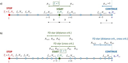
4.2. Monte Carlo approach with meshless random walk

In case an arbitrarily irregular cloud of nodes is used, one may deal with a meshless variant of a random walk, in which all nodes have pre-defined positions. However, both move directions (in multidimensional cases) and a step size (for all dimensions) may float (are locally variable (Figure 1(b))). Moreover, neither mesh structure nor mapping restrictions are required. Therefore, it may be classified as a special type of a floating random walk. However, it cannot be considered as a full-floating random walk due to frozen nodes locations. In other words, each new random walk is constructed on the same combination of possible directions.

The determination of potential move directions should be based upon either distance or cross criterion, with the number of nodes in stars providing well-conditioned schemes, in order to avoid negative probabilities. Afterwards, selection probabilities, assigned to the ith internal node and leading to one of its remaining $m_s-1$ star nodes, may be derived from (24(24) $\{\begin{array}{l}{T}_1\left(\mathbf{P}\right)=T_a,i=1,\\ {\displaystyle \sum _{l=1}^{m_s}({\lambda }_i^{\mathrm{\prime }}{M}_{2,l}\left(x_i\right)+{\lambda }_i{M}_{3,l}\left(x_i\right))T_{l\left(i\right)}\left(\mathbf{P}\right)=-f(x_i,\mathbf{f}),i=2,\dots ,n-1,}\\ {\displaystyle {\lambda }_b\sum _{l=1}^{m_s}{M}_{2,l}\left(x_n\right)T_{l\left(n\right)}\left(\mathbf{P}\right)=q_b,i=n}\end{array}$(24) ), namely (35) $T_i\left(\mathbf{P}\right)=\sum _{l=2}^{m_s}{p}_{l\left(i\right)}{T}_{l\left(i\right)}\left(\mathbf{P}\right)+s_{i}f(x_i,\mathbf{f}),i\in \{2,3,\dots ,n\}$(35) with selection probabilities $p_{l\left(i\right)}$ and the scaling factor $s_i$ equal (36) $p_{l\left(i\right)}=-\frac{{\lambda }_i^{\mathrm{\prime }}{M}_{2,l}\left(x_i\right)+{\lambda }_i{M}_{3,l}\left(x_i\right)}{{\lambda }_i^{\mathrm{\prime }}{M}_{2,1}\left(x_i\right)+{\lambda }_i{M}_{3,1}\left(x_i\right)},s_i=-\frac{1}{{\lambda }_i^{\mathrm{\prime }}{M}_{2,1}\left(x_i\right)+{\lambda }_i{M}_{3,1}\left(x_i\right)}$(36) with $\sum _{l=2}^{m_s}{p}_{l\left(i\right)}=1$. On the contrary to a fixed random walk and according to (24(24) $\{\begin{array}{l}{T}_1\left(\mathbf{P}\right)=T_a,i=1,\\ {\displaystyle \sum _{l=1}^{m_s}({\lambda }_i^{\mathrm{\prime }}{M}_{2,l}\left(x_i\right)+{\lambda }_i{M}_{3,l}\left(x_i\right))T_{l\left(i\right)}\left(\mathbf{P}\right)=-f(x_i,\mathbf{f}),i=2,\dots ,n-1,}\\ {\displaystyle {\lambda }_b\sum _{l=1}^{m_s}{M}_{2,l}\left(x_n\right)T_{l\left(n\right)}\left(\mathbf{P}\right)=q_b,i=n}\end{array}$(24) ), the number of possible move directions at right boundary node ($x_n$) is larger, not pre-defined and dependent on the local star configuration (37) $T_{l\left(n\right)}=\sum _{l=2}^{m_s}{p}_{l\left(n\right)}{T}_{l\left(n\right)}+s_n{q}_b$(37) where (38) $p_{l\left(n\right)}=-\frac{M_{2,l}\left(x_n\right)}{M_{2,1}\left(x_n\right)},s_n=\frac{1}{{\lambda }_b{M}_{2,1}\left(x_n\right)}$(38) Eventually, the final Monte Carlo formula for $T_i$ is the same as already given in (33(33) $\begin{array}{rl}T(x_i,\mathbf{P})& =T_i\left(\mathbf{P}\right)\approx \frac{1}{N}(N_{i,1}{T}_a+\sum _{l=2}^{n-1}{N}_{i,l}{s}_{l}f(x_l,\mathbf{f})+N_{i,n}{s}_n{q}_b)\\ & =T_a+\frac{1}{N}(\sum _{l=2}^{n-1}{N}_{i,l}{s}_{l}f(x_l,\mathbf{f})+N_{i,n}{s}_n{q}_b)\end{array}$(33) ).

4.3. Stochastic approximation of temperature gradient and Hessian matrix

Direct analytical differentiation of (33(33) $\begin{array}{rl}T(x_i,\mathbf{P})& =T_i\left(\mathbf{P}\right)\approx \frac{1}{N}(N_{i,1}{T}_a+\sum _{l=2}^{n-1}{N}_{i,l}{s}_{l}f(x_l,\mathbf{f})+N_{i,n}{s}_n{q}_b)\\ & =T_a+\frac{1}{N}(\sum _{l=2}^{n-1}{N}_{i,l}{s}_{l}f(x_l,\mathbf{f})+N_{i,n}{s}_n{q}_b)\end{array}$(33) ) yields (39) ${\mathbf{\nabla }}_{\mathbf{P}}{T}_i=\left\{\frac{\mathrm{\partial }{T}_i}{\mathrm{\partial }{P}_j}\right\}=\{\begin{array}{l}{\displaystyle \frac{\mathrm{\partial }{T}_i}{\mathrm{\partial }{T}_a}=\frac{N_{i,1}}{N}=1,j=1,}\\ {\displaystyle \frac{\mathrm{\partial }{T}_i}{\mathrm{\partial }{q}_b}=\frac{N_{i,n}{s}_n}{N},j=2,}\\ {\displaystyle \frac{\mathrm{\partial }{T}_i}{\mathrm{\partial }{f}_{j-2}}=\frac{1}{N}\sum _{l=2}^{n-1}{N}_{i,l}{s}_l{\mathrm{\Phi }}_{j-2}\left(x_l\right),3\le j\le m_p}\end{array}i=1,2,\dots ,m_t$(39) and $({\mathbf{H}}_{\mathbf{P}}T{)}_i=\mathbf{0}$. By substituting (33(33) $\begin{array}{rl}T(x_i,\mathbf{P})& =T_i\left(\mathbf{P}\right)\approx \frac{1}{N}(N_{i,1}{T}_a+\sum _{l=2}^{n-1}{N}_{i,l}{s}_{l}f(x_l,\mathbf{f})+N_{i,n}{s}_n{q}_b)\\ & =T_a+\frac{1}{N}(\sum _{l=2}^{n-1}{N}_{i,l}{s}_{l}f(x_l,\mathbf{f})+N_{i,n}{s}_n{q}_b)\end{array}$(33) ) and (39(39) ${\mathbf{\nabla }}_{\mathbf{P}}{T}_i=\left\{\frac{\mathrm{\partial }{T}_i}{\mathrm{\partial }{P}_j}\right\}=\{\begin{array}{l}{\displaystyle \frac{\mathrm{\partial }{T}_i}{\mathrm{\partial }{T}_a}=\frac{N_{i,1}}{N}=1,j=1,}\\ {\displaystyle \frac{\mathrm{\partial }{T}_i}{\mathrm{\partial }{q}_b}=\frac{N_{i,n}{s}_n}{N},j=2,}\\ {\displaystyle \frac{\mathrm{\partial }{T}_i}{\mathrm{\partial }{f}_{j-2}}=\frac{1}{N}\sum _{l=2}^{n-1}{N}_{i,l}{s}_l{\mathrm{\Phi }}_{j-2}\left(x_l\right),3\le j\le m_p}\end{array}i=1,2,\dots ,m_t$(39) ) into (10(10) ${\mathbf{\nabla }}_{\mathbf{P}}F\left(\mathbf{P}\right)=2\sum _{i=1}^{m_t}{\displaystyle \frac{T({\hat{\mathbf{x}}}_i,\mathbf{P})-{\hat{T}}_i}{\mathrm{\Delta }{T}_i^2}}{\mathbf{\nabla }}_{\mathbf{P}}T({\hat{\mathbf{x}}}_i,\mathbf{P})$(10) ) and (12(12) $\begin{array}{rl}{\mathbf{H}}_{\mathbf{P}}F\left(\mathbf{P}\right)& ={\mathbf{\nabla }}_{\mathbf{P}}\otimes \left({\mathbf{\nabla }}_{\mathbf{P}}F\left(\mathbf{P}\right)\right)\\ & =2\sum _{i=1}^{m_t}{\displaystyle \frac{{\mathbf{\nabla }}_{\mathbf{P}}T({\hat{\mathbf{x}}}_i,\mathbf{P}){\mathbf{\nabla }}_{\mathbf{P}}^{\mathrm{\top }}T({\hat{\mathbf{x}}}_i,\mathbf{P})+(T({\hat{\mathbf{x}}}_i,\mathbf{P})-{\hat{T}}_i){\mathbf{H}}_{\mathbf{P}}T({\hat{x}}_i,\mathbf{P})}{\mathrm{\Delta }{T}_i^2}}\end{array}$(12) ), one obtains (40) ${\mathbf{\nabla }}_{\mathbf{P}}F\left(\mathbf{P}\right)=\sum _{i=1}^{m_t}{\displaystyle \frac{T_i\left(\mathbf{P}\right)-{\hat{T}}_i}{\mathrm{\Delta }{T}_i^2}}{\mathbf{\nabla }}_{\mathbf{P}}{T}_i,{\mathbf{H}}_{\mathbf{P}}F=\sum _{i=1}^{m_t}{\displaystyle \frac{{\mathbf{\nabla }}_{\mathbf{P}}{T}_i{\mathbf{\nabla }}_{\mathbf{P}}^{\mathrm{\top }}{T}_i}{\mathrm{\Delta }{T}_i^2}}$(40)

5. Final optimization algorithms

This section concerns the issues of numerical analysis of the primary optimization problem (5(5) ${\mathbf{P}}^{\left(\mathrm{o}\mathrm{p}\mathrm{t}\right)}=\underset{\left(\mathbf{P}\right)}{\mathrm{a}\mathrm{r}\mathrm{g}\mathrm{m}\mathrm{i}\mathrm{n}}F\left(\mathbf{P}\right),F\left(\mathbf{P}\right)=\sqrt{\frac{1}{m_t}\sum _{i=1}^{m_t}{\left({\displaystyle \frac{T({\hat{x}}_i,\mathbf{P})-{\hat{T}}_i}{\mathrm{\Delta }{T}_i}}\right)}^2}$(5) ) which requires multiple solutions of (1(1) $\{\begin{array}{l}T(a,\mathbf{P})=T_a,x=a,\\ -{\displaystyle \frac{\mathrm{d}\lambda }{\mathrm{d}x}}{\displaystyle \frac{\mathrm{\partial }T}{\mathrm{\partial }x}}-\lambda \left(x\right){\displaystyle \frac{{\mathrm{\partial }}^{2}T}{\mathrm{\partial }{x}^2}}=f(x,\mathbf{f}),x\in (a,b)\\ \lambda \left(b\right){\displaystyle \frac{\mathrm{\partial }T}{\mathrm{\partial }x}}(b,\mathbf{P})=q_b,x=b.\end{array}$(1) ), obtained by means of standard FD, meshless FD (Section 3) or Monte Carlo method with various types of random walks (Section 4). The minimum of the objective function F from (5(5) ${\mathbf{P}}^{\left(\mathrm{o}\mathrm{p}\mathrm{t}\right)}=\underset{\left(\mathbf{P}\right)}{\mathrm{a}\mathrm{r}\mathrm{g}\mathrm{m}\mathrm{i}\mathrm{n}}F\left(\mathbf{P}\right),F\left(\mathbf{P}\right)=\sqrt{\frac{1}{m_t}\sum _{i=1}^{m_t}{\left({\displaystyle \frac{T({\hat{x}}_i,\mathbf{P})-{\hat{T}}_i}{\mathrm{\Delta }{T}_i}}\right)}^2}$(5) ), with respect to the vector of decision variables $\mathbf{P}$, and with constraints defined in (6(6) $|T({\hat{x}}_i,\mathbf{P})-{\hat{T}}_i|<\mathrm{\Delta }{T}_i,i=1,2,\dots ,m_t$(6) ), is sought. The objective function relates measured temperatures with temperatures computed for $\mathbf{P}$ which corresponds to the solution of the inverse boundary value problem (1(1) $\{\begin{array}{l}T(a,\mathbf{P})=T_a,x=a,\\ -{\displaystyle \frac{\mathrm{d}\lambda }{\mathrm{d}x}}{\displaystyle \frac{\mathrm{\partial }T}{\mathrm{\partial }x}}-\lambda \left(x\right){\displaystyle \frac{{\mathrm{\partial }}^{2}T}{\mathrm{\partial }{x}^2}}=f(x,\mathbf{f}),x\in (a,b)\\ \lambda \left(b\right){\displaystyle \frac{\mathrm{\partial }T}{\mathrm{\partial }x}}(b,\mathbf{P})=q_b,x=b.\end{array}$(1) ). Therefore, evaluation of temperatures at measurement points, by means of deterministic or stochastic approach, is obligatory for all optimization methods, regardless of their type. Moreover, the evaluation of temperature gradient is required for gradient methods. In this section, computational algorithms of selected, most commonly applied, optimization methods are briefly discussed. Moreover, the proposed direct Monte Carlo optimization approach is presented in a detailed manner.

5.1. Brute-force search

The brute-force search (aka exhaustive search, also known as generate and test approach) is the simplest though computationally demanding, time-consuming and rather inaccurate optimization method. It is based on the analysis of all potential solutions of the optimization problem (5(5) ${\mathbf{P}}^{\left(\mathrm{o}\mathrm{p}\mathrm{t}\right)}=\underset{\left(\mathbf{P}\right)}{\mathrm{a}\mathrm{r}\mathrm{g}\mathrm{m}\mathrm{i}\mathrm{n}}F\left(\mathbf{P}\right),F\left(\mathbf{P}\right)=\sqrt{\frac{1}{m_t}\sum _{i=1}^{m_t}{\left({\displaystyle \frac{T({\hat{x}}_i,\mathbf{P})-{\hat{T}}_i}{\mathrm{\Delta }{T}_i}}\right)}^2}$(5) ) in order to select the optimal one that meets assumed requirements. Therefore, it has practically only historical meaning, nowadays, and may be applied either to low-dimensional optimization problems (i.e. $m_p=1,2$) or to problems for which it is impossible or too difficult to find a solution using other, more accurate methods. Otherwise, computational complexity of the method exceeds capabilities of modern hardware. However, it may be applied as a coarse estimation of the optimal solution, being an initial solution to other, more sophisticated methods. Despite all its drawbacks, it has one important feature that other methods lack, namely it may construct roughly the graph of the objective function, indicating the type of the optimization problem (e.g. the saddle problem, the valley problem, existence of multiple global solutions etc.), which may help to develop more appropriate, problem-driven optimization method.

The required number of the objective function values equals $N_{bfs}^{\left(T\right)}=\prod _{j=1}^{m_p}(n_j+1)$, with $n_j$ being the number of divisions of the searching subspace corresponding to the jth decision variable ($P_j$). After ${\mathbf{P}}^{\left(\mathrm{o}\mathrm{p}\mathrm{t}\right)}$ (for which F in (5(5) ${\mathbf{P}}^{\left(\mathrm{o}\mathrm{p}\mathrm{t}\right)}=\underset{\left(\mathbf{P}\right)}{\mathrm{a}\mathrm{r}\mathrm{g}\mathrm{m}\mathrm{i}\mathrm{n}}F\left(\mathbf{P}\right),F\left(\mathbf{P}\right)=\sqrt{\frac{1}{m_t}\sum _{i=1}^{m_t}{\left({\displaystyle \frac{T({\hat{x}}_i,\mathbf{P})-{\hat{T}}_i}{\mathrm{\Delta }{T}_i}}\right)}^2}$(5) ) reaches its smallest value) is determined, one should examine whether (6(6) $|T({\hat{x}}_i,\mathbf{P})-{\hat{T}}_i|<\mathrm{\Delta }{T}_i,i=1,2,\dots ,m_t$(6) ) are fulfilled. In case they are not, a division refinement of the problem space may be required, or another brute-force search may be performed in the closest neighbourhood of ${\mathbf{P}}^{\left(\mathrm{o}\mathrm{p}\mathrm{t}\right)}$, defined by the actual increment $\mathrm{\Delta }\mathbf{P}$.

5.2. Newton method

The Newton method is a representative among gradient descent methods, which are based upon the iterative numerical solution of the system of non-linear equations (in general), resulting from (9(9) ${\mathbf{\nabla }}_{\mathbf{P}}F\left(\mathbf{P}\right)=\mathbf{0}$(9) ). The subsequent increments $\mathrm{\Delta }{\mathbf{P}}^{(k+1)}$, obtained by means of the solution of the linearized system of equations (41) ${\mathbf{H}}_{\mathbf{P}}F\mathrm{\Delta }{\mathbf{P}}^{(k+1)}=-{\mathbf{\nabla }}_{\mathbf{P}}F\left({\mathbf{P}}^{\left(k\right)}\right)$(41) are used for the solution updating at every kth iteration step (42) ${\mathbf{P}}^{(k+1)}={\mathbf{P}}^{\left(k\right)}+\mathrm{\Delta }{\mathbf{P}}^{(k+1)},k=0,1,\dots ,k_{max}$(42) where $k_{max}$ is the assumed maximum number of iterations. Calculations are carried out as long as (6(6) $|T({\hat{x}}_i,\mathbf{P})-{\hat{T}}_i|<\mathrm{\Delta }{T}_i,i=1,2,\dots ,m_t$(6) ) are fulfilled, either locally or globally, in a mean squared norm. Furthermore, appropriate brake-off test may be examined, based upon estimation of the solution error (43) ${ϵ}_{\mathbf{P}}=\frac{\Vert {\mathbf{P}}^{(k+1)}-{\mathbf{P}}^{\left(k\right)}\Vert }{\Vert {\mathbf{P}}^{(k+1)}\Vert }<{ϵ}_{adm}$(43) where ${ϵ}_{adm}$ is the assumed admissible solution error. Afterwards, ${\mathbf{P}}^{\left(\mathrm{o}\mathrm{p}\mathrm{t}\right)}\approx {\mathbf{P}}^{k_{act}}$, where $k_{act}$ is the actual number of performed iterations.

The Newton method is characterized by the fast quadratic convergence, though it is very sensitive to the initial solution ${\mathbf{P}}^{\left(0\right)}\in {\mathbf{P}}^{\left(adm\right)}$. Moreover, the Hessian matrix has to be evaluated, though only once, due to its constant value (with respect to $\mathbf{P}$). The total number of solutions of boundary value problem equals $N_{Nm}^{\left(T\right)}=m_p+k_{act}(m_p+1)$.

5.3. Method of steepest descent

The operation of the steepest descent method is very similar to the Newton method. First, the initial solution ${\mathbf{P}}^{\left(0\right)}\in {\mathbf{P}}^{\left(adm\right)}$ is selected. At every iteration step, the anti-gradient of the objective function ($-{\mathbf{\nabla }}_{\mathbf{P}}F$) is calculated, which defines the searching direction ${\mathbf{d}}^{\left(k\right)}$ in the admissible solution space, namely (44) ${\mathbf{P}}^{(k+1)}={\mathbf{P}}^{\left(k\right)}+{\alpha }^{\left(k\right)}{\mathbf{d}}^{\left(k\right)}={\mathbf{P}}^{\left(k\right)}-{\alpha }^{\left(k\right)}{\mathbf{\nabla }}_{\mathbf{P}}F\left({\mathbf{P}}^{\left(k\right)}\right),k=0,1,\dots ,k_{max}$(44) where ${\mathbf{d}}^{\left(k\right)}=-{\mathbf{\nabla }}_{\mathbf{P}}F\left({\mathbf{P}}^{\left(k\right)}\right)$. The current step size ${\alpha }^{\left(k\right)}$ is selected by the solution of an auxiliary directional one-dimensional optimization problem (45) ${\alpha }^{\left(k\right)}=\underset{(\alpha >0)}{\mathrm{a}\mathrm{r}\mathrm{g}\mathrm{m}\mathrm{i}\mathrm{n}}F({\mathbf{P}}^{\left(k\right)}+\alpha {\mathbf{d}}^{\left(k\right)})$(45) Among methods of the one-dimensional minimization, one may distinguish the golden section (interval division into two subintervals whose length ratio is the same as the ratio of the total interval length to the longer part), the midpoint (bisection), the dichotomy or Newton methods. In case of bisection method, the admissible interval for α has to be assumed, for instance, $\alpha \in ({\alpha }_a=0,{\alpha }_b={\alpha }_{max})$, where ${\alpha }_{max}$ may correspond to physical dimensions of the original inverse problem, providing the anti-gradient has been normalized ($\Vert {\mathbf{d}}^{\left(k\right)}\Vert =1$). At each iteration step, one has to evaluate the current centre point ${\alpha }_c=0.5({\alpha }_a+{\alpha }_b)$ and as well as the gradient product (46) $G={\mathbf{\nabla }}_{\mathbf{P}}F({\mathbf{P}}^{\left(k\right)}+{\alpha }_a{\mathbf{d}}^{\left(k\right)}){\mathbf{d}}^{\left(k\right)}\cdot {\mathbf{\nabla }}_{\mathbf{P}}F({\mathbf{P}}^{\left(k\right)}+{\alpha }_c{\mathbf{d}}^{\left(k\right)}){\mathbf{d}}^{\left(k\right)}$(46) The sign of (46(46) $G={\mathbf{\nabla }}_{\mathbf{P}}F({\mathbf{P}}^{\left(k\right)}+{\alpha }_a{\mathbf{d}}^{\left(k\right)}){\mathbf{d}}^{\left(k\right)}\cdot {\mathbf{\nabla }}_{\mathbf{P}}F({\mathbf{P}}^{\left(k\right)}+{\alpha }_c{\mathbf{d}}^{\left(k\right)}){\mathbf{d}}^{\left(k\right)}$(46) ) determines which of two subintervals of equal length ($({\alpha }_a,{\alpha }_c)$ or $({\alpha }_c,{\alpha }_b)$) is divided in the subsequent iteration, namely ${\alpha }_b={\alpha }_c$ if G<0, and ${\alpha }_a={\alpha }_c$ otherwise. The appropriate brake-off criterion for bisection method may correspond to the length of $({\alpha }_a,{\alpha }_b)$ interval. Consequently, ${\alpha }^{\left(k\right)}\approx {\alpha }_c$. The external brake-off criterion for (44(44) ${\mathbf{P}}^{(k+1)}={\mathbf{P}}^{\left(k\right)}+{\alpha }^{\left(k\right)}{\mathbf{d}}^{\left(k\right)}={\mathbf{P}}^{\left(k\right)}-{\alpha }^{\left(k\right)}{\mathbf{\nabla }}_{\mathbf{P}}F\left({\mathbf{P}}^{\left(k\right)}\right),k=0,1,\dots ,k_{max}$(44) ) may be the same as for the Newton method, yielding ${\mathbf{P}}^{\left(\mathrm{o}\mathrm{p}\mathrm{t}\right)}\approx {\mathbf{P}}^{\left(k_{act}\right)}$. The steepest descent method is characterized by the linear convergence, much slower than in case of the Newton method, especially when the initial solution is selected in an unfortunate manner. In addition, the method may be very sensitive to rounding errors. The total number of solutions of boundary value problem $N_{msd}^{\left(T\right)}$ strongly depends on the accuracy of the bisection method and may be upper-bounded by $N_{msd}^{\left(T\right)}<k_{act}{k}_{max}(m_p+1{)}^2$.

5.4. Genetic algorithms

Genetic algorithms (GA) are the stochastic search-type optimization approach in which decision variables are coded as binary numbers, with $m_j$ bits for each component of $\mathbf{P}$ ($j=1,2,\dots ,m_p$). The wider group of evolutionary algorithms directly works on decimal (real) numbers, however binary coding seems to be more natural for computers' architecture. Therefore, GA rely on the following parameters, namely the number of members in each genetic population (M), the number of bits for each component of population member ($m_j$) as well as the maximum number of generations ($K_{max}$). Moreover, probabilities of crossover ($p_c=0.6÷0.9$) and mutation ($p_m\le \frac{1}{(m_j+1)\cdot M}=0.1÷0.3$) have to be assumed.

The initial population ${\mathbf{S}}^{\left(0\right)}$, consisting of M members (binary chains) of m bits $\{0,1\}$ each, may be generated randomly. While M is assumed, m is selected as the smallest integer number that satisfies the following inequality (47) $(P_j^{(max)}-P_j^{(min)})\cdot {10}^c\le 2m_j-1$(47) with $c=1,2,3,\dots$, which denotes the number of significant figures of each population member (digits that carry meaning contributing to its measurement resolution). Afterwards, ${\mathbf{P}}^{(k,l)}$ are determined for each lth member belonging to the current binary population ${\mathbf{S}}^{\left(k\right)}$, by means of a simple transformation of binary numbers into decimal ones (48) $P_j^{(k,l)}=P_j^{(min)}+\frac{(P_j^{(max)}-P_j^{(min)})\sum _{i=1}^{m_j}{2}^{i-1}\cdot s_{i\left(j\right)}^{(k,l)}}{2^{m_j}-1},\begin{array}{c}j=1,2,\dots ,m_p,\\ l=1,2,\dots ,M,\\ k=0,1,2,\dots ,K_{max}\end{array}$(48) It is followed by the determination of the objective function (5(5) ${\mathbf{P}}^{\left(\mathrm{o}\mathrm{p}\mathrm{t}\right)}=\underset{\left(\mathbf{P}\right)}{\mathrm{a}\mathrm{r}\mathrm{g}\mathrm{m}\mathrm{i}\mathrm{n}}F\left(\mathbf{P}\right),F\left(\mathbf{P}\right)=\sqrt{\frac{1}{m_t}\sum _{i=1}^{m_t}{\left({\displaystyle \frac{T({\hat{x}}_i,\mathbf{P})-{\hat{T}}_i}{\mathrm{\Delta }{T}_i}}\right)}^2}$(5) ) for each lth member ${\mathbf{P}}^{(k,l)}$ of the current kth population, with temperature values at measurement points obtained by means of either the solution of appropriate SAE (17(17) $\mathbf{T}\left(\mathbf{P}\right)={\mathbf{K}}^{-1}\mathbf{F}\left(\mathbf{P}\right)$(17) ) (for standard and meshless FD analyses) or the explicit Monte Carlo formula (33(33) $\begin{array}{rl}T(x_i,\mathbf{P})& =T_i\left(\mathbf{P}\right)\approx \frac{1}{N}(N_{i,1}{T}_a+\sum _{l=2}^{n-1}{N}_{i,l}{s}_{l}f(x_l,\mathbf{f})+N_{i,n}{s}_n{q}_b)\\ & =T_a+\frac{1}{N}(\sum _{l=2}^{n-1}{N}_{i,l}{s}_{l}f(x_l,\mathbf{f})+N_{i,n}{s}_n{q}_b)\end{array}$(33) ). The current solution population ${\mathbf{S}}^{\left(k\right)}\to {\mathbf{S}}^{(k+1)}$ is consistently proceeded by means of three basic genetic operators, namely (i) selection (of simple roulette type), in which each lth population member is assigned a selection probability (49) $p^{(k,l)}=\frac{F^{-1}\left({\mathbf{P}}^{(k,l)}\right)}{\sum _{i=1}^M{F}^{-1}\left({\mathbf{P}}^{(k,i)}\right)}$(49) which is directly proportional to its contribution to the sum of all objective function (5(5) ${\mathbf{P}}^{\left(\mathrm{o}\mathrm{p}\mathrm{t}\right)}=\underset{\left(\mathbf{P}\right)}{\mathrm{a}\mathrm{r}\mathrm{g}\mathrm{m}\mathrm{i}\mathrm{n}}F\left(\mathbf{P}\right),F\left(\mathbf{P}\right)=\sqrt{\frac{1}{m_t}\sum _{i=1}^{m_t}{\left({\displaystyle \frac{T({\hat{x}}_i,\mathbf{P})-{\hat{T}}_i}{\mathrm{\Delta }{T}_i}}\right)}^2}$(5) ) values; thus, randomly selected members (according to $p_i$ distribution) pass to the next step; (ii) crossover (occurring with $p_c$), in which randomly selected pairs of members $({\mathbf{s}}^{(k,i)},{\mathbf{s}}^{(k,l)})\in {\mathbf{S}}^{\left(k\right)}$ change parts of their chains of bits; and (iii) mutation, in which every bit is assigned a random number $r\in [0,1]$, in accordance with $p_m$; if $r\le p_m$, this particular bit changes from 0 to 1, or from 1 to 0. After each generation, appropriate brake-off criterion has to be examined. It may be based upon the control of the assumed percentage of those members of $\mathbf{P}$ which minimize (5(5) ${\mathbf{P}}^{\left(\mathrm{o}\mathrm{p}\mathrm{t}\right)}=\underset{\left(\mathbf{P}\right)}{\mathrm{a}\mathrm{r}\mathrm{g}\mathrm{m}\mathrm{i}\mathrm{n}}F\left(\mathbf{P}\right),F\left(\mathbf{P}\right)=\sqrt{\frac{1}{m_t}\sum _{i=1}^{m_t}{\left({\displaystyle \frac{T({\hat{x}}_i,\mathbf{P})-{\hat{T}}_i}{\mathrm{\Delta }{T}_i}}\right)}^2}$(5) ). Furthermore, in practical calculations, if there is no solution quality improvement after the specified number of populations, the process stops. Moreover, inequality constraints (6(6) $|T({\hat{x}}_i,\mathbf{P})-{\hat{T}}_i|<\mathrm{\Delta }{T}_i,i=1,2,\dots ,m_t$(6) ) are taken into account.

The final thermal analysis is performed on the basis of the best member of the last determined population ${\mathbf{P}}^{\left(\mathrm{o}\mathrm{p}\mathrm{t}\right)}$. The maximum number of solutions of boundary value problem is $N_{ga}^{\left(T\right)}=M{K}_{max}$.

5.5. Direct Monte Carlo approach

The general Monte Carlo formula (33(33) $\begin{array}{rl}T(x_i,\mathbf{P})& =T_i\left(\mathbf{P}\right)\approx \frac{1}{N}(N_{i,1}{T}_a+\sum _{l=2}^{n-1}{N}_{i,l}{s}_{l}f(x_l,\mathbf{f})+N_{i,n}{s}_n{q}_b)\\ & =T_a+\frac{1}{N}(\sum _{l=2}^{n-1}{N}_{i,l}{s}_{l}f(x_l,\mathbf{f})+N_{i,n}{s}_n{q}_b)\end{array}$(33) ), when introduced to F, defined in (5(5) ${\mathbf{P}}^{\left(\mathrm{o}\mathrm{p}\mathrm{t}\right)}=\underset{\left(\mathbf{P}\right)}{\mathrm{a}\mathrm{r}\mathrm{g}\mathrm{m}\mathrm{i}\mathrm{n}}F\left(\mathbf{P}\right),F\left(\mathbf{P}\right)=\sqrt{\frac{1}{m_t}\sum _{i=1}^{m_t}{\left({\displaystyle \frac{T({\hat{x}}_i,\mathbf{P})-{\hat{T}}_i}{\mathrm{\Delta }{T}_i}}\right)}^2}$(5) ), offers a possibility of a direct differentiation of temperature function with respect to unknown load parameters (2(2) $\mathbf{P}=[T_a,q_b,{\mathbf{f}}^{\mathrm{\top }}]=[T_a,q_b,f_1,f_2,\dots ,f_{m_f}]$(2) ). In such a manner, no numerical optimization approach is required and the method becomes self-starting. One needs neither an initial guess solution, required for Newton and the steepest descent methods, nor admissible intervals (7(7) $\mathbf{P}\in {\mathbf{P}}^{\left(adm\right)}=[{\mathbf{P}}^{(min)},{\mathbf{P}}^{(max)}]$(7) ), required for brute-search and genetic algorithms approaches. Moreover, no iterative procedure is involved, as the resulting system of $m_p$ equations with $m_p$ unknowns is linear and may be solved analytically, or using standard elimination methods.

After substitution of (33(33) $\begin{array}{rl}T(x_i,\mathbf{P})& =T_i\left(\mathbf{P}\right)\approx \frac{1}{N}(N_{i,1}{T}_a+\sum _{l=2}^{n-1}{N}_{i,l}{s}_{l}f(x_l,\mathbf{f})+N_{i,n}{s}_n{q}_b)\\ & =T_a+\frac{1}{N}(\sum _{l=2}^{n-1}{N}_{i,l}{s}_{l}f(x_l,\mathbf{f})+N_{i,n}{s}_n{q}_b)\end{array}$(33) ) into F from (5(5) ${\mathbf{P}}^{\left(\mathrm{o}\mathrm{p}\mathrm{t}\right)}=\underset{\left(\mathbf{P}\right)}{\mathrm{a}\mathrm{r}\mathrm{g}\mathrm{m}\mathrm{i}\mathrm{n}}F\left(\mathbf{P}\right),F\left(\mathbf{P}\right)=\sqrt{\frac{1}{m_t}\sum _{i=1}^{m_t}{\left({\displaystyle \frac{T({\hat{x}}_i,\mathbf{P})-{\hat{T}}_i}{\mathrm{\Delta }{T}_i}}\right)}^2}$(5) ), one obtains the following formula for F, namely (50) $F\left(\mathbf{P}\right)=\sqrt{\frac{1}{m_t}\sum _{i=1}^{m_t}{\displaystyle \frac{1}{\mathrm{\Delta }{T}_i^2}}{(T_a+\frac{1}{N}(\sum _{l=2}^{n-1}{N}_{i,l}{s}_{l}f(x_l,\mathbf{f})+N_{i,n}{s}_n{q}_b)-{\hat{T}}_i)}^2}$(50) Assuming that all $\mathrm{\Delta }{T}_i=\mathrm{\Delta }T$ are equal, the gradient of the objective function may be analytically computed, as follows (51) ${\mathbf{\nabla }}_{\mathbf{P}}F\left(\mathbf{P}\right)=\{\begin{array}{l}{\displaystyle \frac{\mathrm{\partial }F}{\mathrm{\partial }{T}_a}=2\sum _{i=1}^{m_t}(T_a+\frac{1}{N}(\sum _{l=2}^{n-1}{N}_{i,l}{s}_{l}f(x_l,\mathbf{f})+N_{i,n}{s}_n{q}_b)-{\hat{T}}_i)m_t}\\ {\displaystyle \frac{\mathrm{\partial }F}{\mathrm{\partial }{q}_b}=2\sum _{i=1}^{m_t}(T_a+\frac{1}{N}(\sum _{l=2}^{n-1}{N}_{i,l}{s}_{l}f(x_l,\mathbf{f})+N_{i,n}{s}_n{q}_b)-{\hat{T}}_i)\frac{s_n}{N}\sum _{i=1}^{m_t}{N}_{i,n}}\\ {\displaystyle \frac{\mathrm{\partial }F}{\mathrm{\partial }{f}_{j-2}}=2\sum _{i=1}^{m_t}(T_a+\frac{1}{N}(\sum _{l=2}^{n-1}{N}_{i,l}{s}_{l}f(x_l,\mathbf{f})+N_{i,n}{s}_n{q}_b)-{\hat{T}}_i)\cdot }\\ {\displaystyle \cdot \frac{1}{N}\sum _{i=1}^{m_t}\sum _{l=2}^{n-1}{N}_{j,l}{s}_l{\mathrm{\Phi }}_{j-2}\left(x_l\right),3\le j\le m_f}\end{array}$(51) The fulfillment of the necessary condition (9(9) ${\mathbf{\nabla }}_{\mathbf{P}}F\left(\mathbf{P}\right)=\mathbf{0}$(9) ) leads to the linear system of algebraic equations. Let us distinguish two variants, concerning the heat source function f. In case the heat source function $f=f\left(x\right)$ is known, the only unknown load parameters may be $T_a$ and/or $q_b$. After analytical differentiation of (50(50) $F\left(\mathbf{P}\right)=\sqrt{\frac{1}{m_t}\sum _{i=1}^{m_t}{\displaystyle \frac{1}{\mathrm{\Delta }{T}_i^2}}{(T_a+\frac{1}{N}(\sum _{l=2}^{n-1}{N}_{i,l}{s}_{l}f(x_l,\mathbf{f})+N_{i,n}{s}_n{q}_b)-{\hat{T}}_i)}^2}$(50) ) with respect to $[T_a,q_b{]}^{\mathrm{\top }}$, one obtains the following system of two equations (52) $\left[\begin{array}{cc}{\displaystyle m_t}& {\displaystyle \frac{s_n}{N}\sum _{i=1}^{m_t}{N}_{i,n}}\\ {\displaystyle \frac{s_n}{N}\sum _{i=1}^{m_t}{N}_{i,n}}& {\displaystyle \frac{s_n^2}{N^2}\sum _{i=1}^{m_t}{N}_{i,n}^2}\end{array}\right]\left[\begin{array}{c}{T}_a\\ q_b\end{array}\right]=\left[\begin{array}{c}{\displaystyle \sum _{i=1}^{m_t}({\hat{T}}_i+\frac{1}{N}\sum _{l=2}^{n-1}{N}_{i,l}{s}_{l}f\left(x_l\right))}\\ {\displaystyle \frac{1}{N}\sum _{i=1}^{m_t}(N_{i,n}{s}_n{\hat{T}}_i+\frac{N_{i,n}{s}_n}{N}\sum _{l=2}^{n-1}{N}_{i,l}{s}_{l}f\left(x_l\right))}\end{array}\right]$(52) Depending on the number of unknown load parameters, the final semi-analytical formulas may be determined. The first variant assumes unknown $T_a$ and known $q_b$ (53) $T_a=\frac{1}{N{m}_t}\sum _{i=1}^{m_t}(N{\hat{T}}_i+\sum _{l=2}^{n-1}{N}_{i,l}{s}_{l}f\left(x_l\right)-q_b{N}_{i,n}{s}_n)$(53) while the second one assumes known $T_a$ and unknown $q_b$ (54) $q_b={\left(s_n\sum _{i=1}^{m_t}{N}_{i,n}\right)}^{-1}(\sum _{i=1}^{m_t}(N{\hat{T}}_i+\sum _{l=2}^{n-1}{N}_{i,l}{s}_{l}f\left(x_l\right))-N{m}_t{T}_a)$(54) Otherwise, both $T_a$ and $q_b$ are unknown and may be derived as (55) $\begin{array}{rl}{T}_a& ={\left(N(m_t\sum _{i=1}^{m_t}{N}_{i,n}^2-{\left(\sum _{i=1}^{m_t}{N}_{i,n}\right)}^2)\right)}^{-1}(\sum _{i=1}^{m_t}(N{\hat{T}}_i+\sum _{l=2}^{n-1}{N}_{i,l}{s}_{l}f\left(x_l\right))\sum _{i=1}^{m_t}{N}_{i,n}^2\\ & +-\sum _{i=1}^{m_t}(N{N}_{i,n}{\hat{T}}_i+N_{i,n}\sum _{l=2}^{n-1}{N}_{i,l}{s}_{l}f\left(x_l\right))\sum _{i=1}^{m_t}{N}_{i,n})\end{array}$(55) and (56) $\begin{array}{rl}{q}_b& ={\left(s_n(m_t\sum _{i=1}^{m_t}{N}_{i,n}^2-{\left(\sum _{i=1}^{m_t}{N}_{i,n}\right)}^2)\right)}^{-1}(m_t\sum _{i=1}^{m_t}(N{N}_{i,n}{\hat{T}}_i+N_{i,n}\sum _{l=2}^{n-1}{N}_{i,l}{s}_{l}f\left(x_l\right))\\ & +-\sum _{i=1}^{m_t}{N}_{i,n}\sum _{i=1}^{m_t}(N{\hat{T}}_i+\sum _{l=2}^{n-1}{N}_{i,l}{s}_{l}f\left(x_l\right)))\end{array}$(56) In case the heat source function $f=f\left(x\right)$ is unknown, it has to be approximated using (3(3) $f(x,\mathbf{f})=\sum _{j=1}^{m_f}{\mathrm{\Phi }}_j\left(x\right)f_j=\mathbf{\Phi }\left(x\right)\mathbf{f}$(3) ). After analytical differentiation of (50(50) $F\left(\mathbf{P}\right)=\sqrt{\frac{1}{m_t}\sum _{i=1}^{m_t}{\displaystyle \frac{1}{\mathrm{\Delta }{T}_i^2}}{(T_a+\frac{1}{N}(\sum _{l=2}^{n-1}{N}_{i,l}{s}_{l}f(x_l,\mathbf{f})+N_{i,n}{s}_n{q}_b)-{\hat{T}}_i)}^2}$(50) ) with respect to $\mathbf{P}$, one obtains the following system of $m_p$ equations and $m_p$ unknowns (57) $\mathbf{A}\mathbf{P}=\mathbf{B}\left(\hat{\mathbf{T}}\right)$(57) in which the coefficient matrix $\mathbf{A}$ is defined as (58) $\left[\begin{array}{cccccc}{\displaystyle m_t}& {\displaystyle \frac{s_n}{N}\sum _{i=1}^{m_t}{N}_{i,n}}& {\displaystyle m_t\sum _{i=1}^{m_t}{S}_{i,1}}& {\displaystyle m_t\sum _{i=1}^{m_t}{S}_{i,2}}& \cdots & {\displaystyle m_t\sum _{i=1}^{m_t}{S}_{i,m_f}}\\ {\displaystyle \frac{s_n}{N}\sum _{i=1}^{m_t}{N}_{i,n}}& {\displaystyle \frac{s_n^2}{N^2}\sum _{i=1}^{m_t}{N}_{i,n}^2}& {\displaystyle s_n\sum _{i=1}^{m_t}{N}_{i,n}{S}_{i,1}}& {\displaystyle s_n\sum _{i=1}^{m_t}{N}_{i,n}{S}_{i,2}}& \cdots & {\displaystyle s_n\sum _{i=1}^{m_t}{N}_{i,n}{S}_{i,m_f}}\\ {\displaystyle m_t\sum _{i=1}^{m_t}{S}_{i,1}}& {\displaystyle s_n\sum _{i=1}^{m_t}{N}_{i,n}{S}_{i,1}}& {\displaystyle \sum _{i=1}^{m_t}{S}_{i,1}^2}& {\displaystyle \sum _{i=1}^{m_t}{S}_{i,1}{S}_{i,2}}& \cdots & {\displaystyle \sum _{i=1}^{m_t}{S}_{i,1}{S}_{i,m_f}}\\ {\displaystyle m_t\sum _{i=1}^{m_t}{S}_{i,2}}& {\displaystyle s_n\sum _{i=1}^{m_t}{N}_{i,n}{S}_{i,2}}& {\displaystyle \sum _{i=1}^{m_t}{S}_{i,1}{S}_{i,2}}& {\displaystyle \sum _{i=1}^{m_t}{S}_{i,2}^2}& \cdots & {\displaystyle \sum _{i=1}^{m_t}{S}_{i,2}{S}_{i,m_f}}\\ {\displaystyle \cdots }& \cdots & \cdots & \cdots & \cdots & \cdots \\ {\displaystyle m_t\sum _{i=1}^{m_t}{S}_{i,m_f}}& {\displaystyle s_n\sum _{i=1}^{m_t}{N}_{i,n}{S}_{i,m_f}}& {\displaystyle \sum _{i=1}^{m_t}{S}_{i,m_f}{S}_{i,1}}& {\displaystyle \sum _{i=1}^{m_t}{S}_{i,m_f}{S}_{i,2}}& \cdots & {\displaystyle \sum _{i=1}^{m_t}{S}_{i,m_f}^2}\end{array}\right]$(58) whereas the right-hand side vector, which includes the measured temperatures, is (59) $\mathbf{B}\left(\hat{\mathbf{T}}\right)={\left[\begin{array}{cccccc}{\displaystyle \sum _{i=1}^{m_t}{\hat{T}}_i}& \frac{s_n}{N}\sum _{i=1}^{m_t}{N}_{i,n}{\hat{T}}_i& {\displaystyle \sum _{i=1}^{m_t}{\hat{T}}_i{S}_{i,1}}& {\displaystyle \sum _{i=1}^{m_t}{\hat{T}}_i{S}_{i,2}}& \cdots & {\displaystyle \sum _{i=1}^{m_t}{\hat{T}}_i{S}_{i,m_f}}\end{array}\right]}^{\mathrm{\top }}$(59) in which (60) $S_{i,j}=-\frac{1}{N}\sum _{l=2}^{n-1}{N}_{i,l}{s}_l{\mathrm{\Phi }}_j\left(x_l\right),i=1,2,\dots ,m_t,j=1,2,\dots ,m_f$(60) The above system of equations corresponds to the most general inverse two-point thermal problem, in which all load parameters are unknown. However, in case one or two boundary load parameters are known, this system has to be slightly rebuilt in order to assume known load values. The modified right-hand side vector $\overline{\mathbf{B}}=\mathbf{B}-\mathbf{A}\overline{\mathbf{P}}$ includes vector $\overline{\mathbf{P}}$ of known load parameters and zeros elsewhere. Afterwards, one has to cross out those rows and columns of (57(57) $\mathbf{A}\mathbf{P}=\mathbf{B}\left(\hat{\mathbf{T}}\right)$(57) ) which correspond to known load parameters. For instance, assuming that both $T_a$ and $q_b$ are known as well as $m_f=3$ in (3(3) $f(x,\mathbf{f})=\sum _{j=1}^{m_f}{\mathrm{\Phi }}_j\left(x\right)f_j=\mathbf{\Phi }\left(x\right)\mathbf{f}$(3) ) (i.e. the unknown heat source function is approximated by means of three nodal values and three basis functions), one obtains the following system of equations (61) $\left[\begin{array}{ccc}{\displaystyle \sum _{i=1}^{m_t}{S}_{i,1}^2}& {\displaystyle \sum _{i=1}^{m_t}{S}_{i,1}{S}_{i,2}}& {\displaystyle \sum _{i=1}^{m_t}{S}_{i,1}{S}_{i,3}}\\ {\displaystyle \sum _{i=1}^{m_t}{S}_{i,2}{S}_{i,1}}& {\displaystyle \sum _{i=1}^{m_t}{S}_{i,2}^2}& {\displaystyle \sum _{i=1}^{m_t}{S}_{i,2}{S}_{i,3}}\\ {\displaystyle \sum _{i=1}^{m_t}{S}_{i,3}{S}_{i,1}}& {\displaystyle \sum _{i=1}^{m_t}{S}_{i,3}{S}_{i,2}}& {\displaystyle \sum _{i=1}^{m_t}{S}_{i,3}^2}\end{array}\right]\left[\begin{array}{c}{f}_1\\ f_2\\ f_3\end{array}\right]=\left[\begin{array}{c}{\displaystyle \sum _{i=1}^{m_t}{S}_{i,1}({\hat{T}}_i-m_t{T}_a-s_n{N}_{i,n}{q}_b)}\\ {\displaystyle \sum _{i=1}^{m_t}{S}_{i,2}({\hat{T}}_i-m_t{T}_a-s_n{N}_{i,n}{q}_b)}\\ {\displaystyle \sum _{i=1}^{m_t}{S}_{i,3}({\hat{T}}_i-m_t{T}_a-s_n{N}_{i,n}{q}_b)}\end{array}\right]$(61) Regardless of the load variant, the vector of load parameters $\mathbf{P}$ is uncoupled with both the coefficient matrix and the right-hand side vector. This useful feature, guaranteeing the solution stability, does not hold in case of standard optimization methods, applied to load identification problems. Moreover, the final solution quality depends on three fundamental parameters, namely

• stochastic ones, namely the number of random walks N,

• deterministic ones, namely the number and distribution of nodes n, in a FD mesh / cloud of nodes,

• measurement ones, namely the number $m_t$ as well as locations $\hat{\mathbf{x}}$ of temperature measurements.

among which the proper selection of discretization parameters seems to be of crucial importance. Since the solution obtained by means of the direct Monte Carlo method corresponds to the exact solution of (2), within the assumed numerical model of (1(1) $\{\begin{array}{l}T(a,\mathbf{P})=T_a,x=a,\\ -{\displaystyle \frac{\mathrm{d}\lambda }{\mathrm{d}x}}{\displaystyle \frac{\mathrm{\partial }T}{\mathrm{\partial }x}}-\lambda \left(x\right){\displaystyle \frac{{\mathrm{\partial }}^{2}T}{\mathrm{\partial }{x}^2}}=f(x,\mathbf{f}),x\in (a,b)\\ \lambda \left(b\right){\displaystyle \frac{\mathrm{\partial }T}{\mathrm{\partial }x}}(b,\mathbf{P})=q_b,x=b.\end{array}$(1) ), the inequality constraints (6(6) $|T({\hat{x}}_i,\mathbf{P})-{\hat{T}}_i|<\mathrm{\Delta }{T}_i,i=1,2,\dots ,m_t$(6) ) are a-priori satisfied.

However, the total error of the optimal solution ${\mathbf{P}}^{\left(\mathrm{o}\mathrm{p}\mathrm{t}\right)}$ may be highly influenced by both measurement uncertainties as well as component modelling errors, corresponding to aforementioned stochastic and deterministic parameters. Therefore, the appropriate upper and lower error bounds (${\mathbf{P}}^{\left(\mathrm{u}\mathrm{p}\mathrm{p}\mathrm{e}\mathrm{r}\right)}$ and ${\mathbf{P}}^{\left(\mathrm{l}\mathrm{o}\mathrm{w}\mathrm{e}\mathrm{r}\right)}$, respectively), corresponding to measurement tolerance $\mathrm{\Delta }T$, may be estimated as well, providing the modelling errors are removed or significantly reduced. It may be achieved by means of the following techniques, namely

• the stochastic (N-type) error may be a-priori estimated using formula (34(34) $e<\frac{1}{\sqrt{N}}$(34) ); however this is not the error estimation in the strict (deterministic) sense and should be considered rather as the most probable case for the fixed N; since results for the single N random walk simulation may be inaccurate, the remedy is to perform simulations in series, either averaging indication numbers for various N simulations leading to one single solution of (57(57) $\mathbf{A}\mathbf{P}=\mathbf{B}\left(\hat{\mathbf{T}}\right)$(57) ), or averaging the multiple solutions of (57(57) $\mathbf{A}\mathbf{P}=\mathbf{B}\left(\hat{\mathbf{T}}\right)$(57) ), each for different N simulation,

• the deterministic error ($\Vert e\Vert <C{h}^{p-1}$), including discretization (h-type) and approximation (p-type) parameters and the constant C, independent from h and p, may be controlled and minimized by the generation of the final computational model before the relevant inverse analysis is initialized; this may include non-adaptive regular mesh refinement or generation of adaptive strongly irregular clouds of nodes, which distribution corresponds to selected criteria, for instance minimization of the estimated solution error; therefore it usually requires additional a-posteriori error estimation techniques, like local, global or goal-oriented estimators;

In such a manner, the error bounds of the optimal solution, corresponding to the assumed measurement tolerance, may be estimated without any difficulties by means of two additional solutions of (57(57) $\mathbf{A}\mathbf{P}=\mathbf{B}\left(\hat{\mathbf{T}}\right)$(57) ) for $(\hat{\mathbf{T}}-\mathrm{\Delta }\mathbf{T})$ and $(\hat{\mathbf{T}}+\mathrm{\Delta }\mathbf{T})$, namely (62) ${\mathbf{P}}^{\left(\mathrm{l}\mathrm{o}\mathrm{w}\mathrm{e}\mathrm{r}\right)}={\mathbf{A}}^{-1}\mathbf{B}(\hat{\mathbf{T}}-\mathrm{\Delta }\mathbf{T}),{\mathbf{P}}^{\left(\mathrm{u}\mathrm{p}\mathrm{p}\mathrm{e}\mathrm{r}\right)}={\mathbf{A}}^{-1}\mathbf{B}(\hat{\mathbf{T}}+\mathrm{\Delta }\mathbf{T})$(62) and consequently (63) ${\mathbf{P}}^{\left(\mathrm{o}\mathrm{p}\mathrm{t}\right)}\in \left[\begin{array}{cc}{\mathbf{P}}^{\left(\mathrm{l}\mathrm{o}\mathrm{w}\mathrm{e}\mathrm{r}\right)}& {\mathbf{P}}^{\left(\mathrm{u}\mathrm{p}\mathrm{p}\mathrm{e}\mathrm{r}\right)}\end{array}\right]$(63) where $\mathrm{\Delta }\mathbf{T}$ is the vector collecting measurement tolerances of all $m_t$ measurements.

6. Numerical examples

The proposed Monte Carlo algorithm with fixed (regular meshes) and meshless (irregular clouds of nodes) random walks has been examined on a variety of benchmark examples with simulated measurement data. Two variants of its application to the identification problem of thermal load have been carried out, namely

• as a coupling with standard optimization methods; in that case, the MC solution approach allows for the fast and effective determination of temperatures at measurement points, and

• as a self-determinative solution approach, yielding a solution to an inverse problem in a direct and explicit manner.

Results obtained for both variants are compared with those obtained using numerical models based upon FDM/MFDM and standard optimization methods. The most interesting aspects of such comparisons are influence of a number of random walks N, number of decision variables $m_p$, number of measurements $m_t$ and their locations $\hat{\mathbf{x}}$, number of nodes n as well as computational (CPU) times, which include all computational parts of algorithms, excluding the generation of graphical results, namely

• for standard optimization methods based upon FD or meshless FD methods, CPU times include the mesh generation, construction of the coefficient matrix $\mathbf{K}$ of (15(15) $\mathbf{K}\mathbf{T}\left(\mathbf{P}\right)=\mathbf{F}\left(\mathbf{P}\right)$(15) ) as well as the iteration/searching procedure; it corresponds to the numerical solution of the optimization problem with multiple solutions of algebraic problems (17(17) $\mathbf{T}\left(\mathbf{P}\right)={\mathbf{K}}^{-1}\mathbf{F}\left(\mathbf{P}\right)$(17) ) with the same $\mathbf{K}$ and different thermal load vectors $\mathbf{F}\left(\mathbf{P}\right)$ (which is the most time consuming part of the entire process),

• for standard optimization methods based upon Monte Carlo technique, CPU times include the mesh generation, construction of random walks for measurement points and determination of nodal indication numbers as well as the iteration/searching procedure; it corresponds to the numerical solution of the optimization problem with multiple applications of the final Monte Carlo formula (33(33) $\begin{array}{rl}T(x_i,\mathbf{P})& =T_i\left(\mathbf{P}\right)\approx \frac{1}{N}(N_{i,1}{T}_a+\sum _{l=2}^{n-1}{N}_{i,l}{s}_{l}f(x_l,\mathbf{f})+N_{i,n}{s}_n{q}_b)\\ & =T_a+\frac{1}{N}(\sum _{l=2}^{n-1}{N}_{i,l}{s}_{l}f(x_l,\mathbf{f})+N_{i,n}{s}_n{q}_b)\end{array}$(33) ) (which remains the most time consuming part of the entire process, though it does not require a single solution of system of equations therefore it is relatively much faster than in previous case),

• for the direct Monte Carlo optimization method, CPU time includes the mesh generation, construction of random walks for measurement points and determination of nodal indication numbers (the most time consuming part, although almost negligible) as well as single generation and solution of small system of Equations (57(57) $\mathbf{A}\mathbf{P}=\mathbf{B}\left(\hat{\mathbf{T}}\right)$(57) ).

All computations were performed using the original author's software, written in Matlab R2018a, and run on Intel Core CPU, 180 GHz with 16 GB RAM. It has to emphasized that the operation of random walks may be implemented using various techniques, for instance the use of traditional nested loops with known (N random walks) and unknown number of iterations (from interior to boundary), typical for low-level programming languages. However, this traditional approach may be ineffective, especially in case of 2-point boundary value problem for which there is only one (left) point which terminates all random walks (x = a). Therefore, capabilities of higher-level programming environments (like Matlab) should be applied, for instance full matrix notation and built-in functions operating on vectors, without referring to their individual elements.

6.1. Preliminary example

For illustrative purposes, let us consider the original inverse problem (1(1) $\{\begin{array}{l}T(a,\mathbf{P})=T_a,x=a,\\ -{\displaystyle \frac{\mathrm{d}\lambda }{\mathrm{d}x}}{\displaystyle \frac{\mathrm{\partial }T}{\mathrm{\partial }x}}-\lambda \left(x\right){\displaystyle \frac{{\mathrm{\partial }}^{2}T}{\mathrm{\partial }{x}^2}}=f(x,\mathbf{f}),x\in (a,b)\\ \lambda \left(b\right){\displaystyle \frac{\mathrm{\partial }T}{\mathrm{\partial }x}}(b,\mathbf{P})=q_b,x=b.\end{array}$(1) ) in a simplified form, namely find such temperature function $T=T(x,c)$ that satisfies the following equation with mixed boundary conditions (64) $-\frac{{\mathrm{\partial }}^{2}T}{\mathrm{\partial }{x}^2}=c,x\in (0,1),T(0,c)=0,\frac{\mathrm{\partial }T}{\mathrm{\partial }x}(1,c)=0$(64) with known $m_t$ temperature measurements (4(4) ${\hat{T}}_i\pm \mathrm{\Delta }{T}_i,i=1,2,\dots ,m_t$(4) ) and measurement tolerance $\mathrm{\Delta }T$. Only one load parameter c, corresponding to the constant heat source intensity, is unknown.

Since the problem (64(64) $-\frac{{\mathrm{\partial }}^{2}T}{\mathrm{\partial }{x}^2}=c,x\in (0,1),T(0,c)=0,\frac{\mathrm{\partial }T}{\mathrm{\partial }x}(1,c)=0$(64) ) is trivial, its direct solution may be obtained by means of its analytical integration, namely (65) $T(x,c)=-c\frac{x^2}{2}+cx$(65) The inverse problem may be formulated in terms of the optimization problem with the objective function $F=F\left(c\right)$ from (5(5) ${\mathbf{P}}^{\left(\mathrm{o}\mathrm{p}\mathrm{t}\right)}=\underset{\left(\mathbf{P}\right)}{\mathrm{a}\mathrm{r}\mathrm{g}\mathrm{m}\mathrm{i}\mathrm{n}}F\left(\mathbf{P}\right),F\left(\mathbf{P}\right)=\sqrt{\frac{1}{m_t}\sum _{i=1}^{m_t}{\left({\displaystyle \frac{T({\hat{x}}_i,\mathbf{P})-{\hat{T}}_i}{\mathrm{\Delta }{T}_i}}\right)}^2}$(5) ) and one decision variable c, namely (66) $F\left(c\right)=\sqrt{\frac{1}{m_t}\sum _{i=1}^{m_t}{(T({\hat{x}}_i,c)-{\hat{T}}_i)}^2}=\sqrt{\frac{1}{m_t}\sum _{i=1}^{m_t}{(-c\frac{{\hat{x}}_i}{2}+c{\hat{x}}_i-{\hat{T}}_i)}^2}$(66) Due to its simplicity, F may be analytically differentiated with respect to c, resulting in one linear equation $\frac{\mathrm{d}F}{\mathrm{d}c}=0$, whose solution is (67) $c=\sum _{i=1}^{m_t}{({\hat{x}}_i-0.5{\hat{x}}_i^2)}^2{\left(\sum _{i=1}^{m_t}{\hat{T}}_i({\hat{x}}_i-0.5{\hat{x}}_i^2)\right)}^{-1}$(67) For the direct Monte Carlo approach, the regular mesh of n nodes has to be generated, with modulus $h=\frac{1}{n-1}$. Furthermore, N fixed random walks need to be constructed at all $m_t$ measurement locations. On the basis of (33(33) $\begin{array}{rl}T(x_i,\mathbf{P})& =T_i\left(\mathbf{P}\right)\approx \frac{1}{N}(N_{i,1}{T}_a+\sum _{l=2}^{n-1}{N}_{i,l}{s}_{l}f(x_l,\mathbf{f})+N_{i,n}{s}_n{q}_b)\\ & =T_a+\frac{1}{N}(\sum _{l=2}^{n-1}{N}_{i,l}{s}_{l}f(x_l,\mathbf{f})+N_{i,n}{s}_n{q}_b)\end{array}$(33) ), (30(30) $p_{i-1}=\frac{1}{2}-\frac{h{\lambda }_i^{\mathrm{\prime }}}{4{\lambda }_i},p_{i+1}=\frac{1}{2}+\frac{h{\lambda }_i^{\mathrm{\prime }}}{4{\lambda }_i},s_i=\frac{h^2}{2{\lambda }_i}$(30) ) and (32(32) $p_n=1,s_n=\frac{h}{{\lambda }_b}$(32) ), one has $\lambda =1$, ${\lambda }^{\prime }=0$, temperature estimation (68) $T({\hat{x}}_i,c)=\frac{c{h}^2}{2N}\sum _{l=2}^{n-1}{N}_{i,l},i=1,2,\dots ,m_t$(68) as well as probabilities $p_{i-1}=p_{i+1}=\frac{1}{2}$ and $p_n=1$. Substitution of (68(68) $T({\hat{x}}_i,c)=\frac{c{h}^2}{2N}\sum _{l=2}^{n-1}{N}_{i,l},i=1,2,\dots ,m_t$(68) ) into F from (66(66) $F\left(c\right)=\sqrt{\frac{1}{m_t}\sum _{i=1}^{m_t}{(T({\hat{x}}_i,c)-{\hat{T}}_i)}^2}=\sqrt{\frac{1}{m_t}\sum _{i=1}^{m_t}{(-c\frac{{\hat{x}}_i}{2}+c{\hat{x}}_i-{\hat{T}}_i)}^2}$(66) ) instead of (65(65) $T(x,c)=-c\frac{x^2}{2}+cx$(65) ), and the exact differentiation of F with respect to c yield the following stochastic type estimation formula for c, namely (69) $c=\frac{h^2}{2N}\sum _{i=1}^{m_t}{\left(\sum _{l=2}^{n-1}{N}_{i,l}\right)}^2{\left(\sum _{i=1}^{m_t}{\hat{T}}_i\sum _{l=2}^{n-1}{N}_{i,l}\right)}^{-1}$(69) Temperature measurements are simulated on the basis of manufactured solution (65(65) $T(x,c)=-c\frac{x^2}{2}+cx$(65) ) with assumed c = −2, and then randomly disturbed with $\mathrm{\Delta }T=0.5$. Measurement locations, initially regularly spaced ${\hat{x}}_i=i{h}_t$, with $i=1,2,\dots ,m_t$ and $h_t=\frac{1}{m_t+1}$, are adapted to corresponding $m_t<n$ nodes locations $x_i$ with $i=2,3,\dots ,n-1$. Therefore, measurement points are located irregularly inside the domain, excluding boundary points.

First, fixed parameters $m_t=2$, n = 33 and N = 1000 are assumed, which allows for a-priori estimation of approximation (${10}^{-4}$ for interior, ${10}^{-2}$ for boundary) and stochastic (${10}^{-2}$) errors. 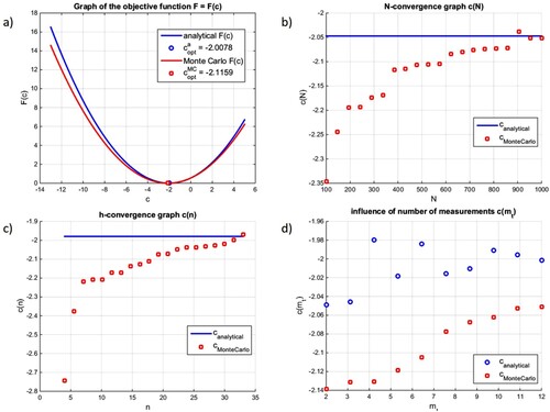The MC formula (69(69) $c=\frac{h^2}{2N}\sum _{i=1}^{m_t}{\left(\sum _{l=2}^{n-1}{N}_{i,l}\right)}^2{\left(\sum _{i=1}^{m_t}{\hat{T}}_i\sum _{l=2}^{n-1}{N}_{i,l}\right)}^{-1}$(69) ), though convergent to (67(67) $c=\sum _{i=1}^{m_t}{({\hat{x}}_i-0.5{\hat{x}}_i^2)}^2{\left(\sum _{i=1}^{m_t}{\hat{T}}_i({\hat{x}}_i-0.5{\hat{x}}_i^2)\right)}^{-1}$(67) ), is influenced by errors of both types. However, in order to avoid convergence of non-uniform stochastic type, random walks are performed in 10 series, with additional averaging of intermediate results. Comparison of graphs of the objective function, obtained using two approaches (analytical and Monte Carlo formulae) as well as optimal c's for both methods are presented in Figure 2(a). In Figure 2(b), results of N-convergence of c (69(69) $c=\frac{h^2}{2N}\sum _{i=1}^{m_t}{\left(\sum _{l=2}^{n-1}{N}_{i,l}\right)}^2{\left(\sum _{i=1}^{m_t}{\hat{T}}_i\sum _{l=2}^{n-1}{N}_{i,l}\right)}^{-1}$(69) ) are presented, obtained for the fixed $m_t=2$, n = 33 and N varying from 100 to 1000, compared with c from (67(67) $c=\sum _{i=1}^{m_t}{({\hat{x}}_i-0.5{\hat{x}}_i^2)}^2{\left(\sum _{i=1}^{m_t}{\hat{T}}_i({\hat{x}}_i-0.5{\hat{x}}_i^2)\right)}^{-1}$(67) ) (independent of N). In Figure 2(c), results of h-convergence of c from (69(69) $c=\frac{h^2}{2N}\sum _{i=1}^{m_t}{\left(\sum _{l=2}^{n-1}{N}_{i,l}\right)}^2{\left(\sum _{i=1}^{m_t}{\hat{T}}_i\sum _{l=2}^{n-1}{N}_{i,l}\right)}^{-1}$(69) ) are presented, obtained for the fixed $m_t=2$, N = 1000 and n varying from 5 to 33, compared with c from (67(67) $c=\sum _{i=1}^{m_t}{({\hat{x}}_i-0.5{\hat{x}}_i^2)}^2{\left(\sum _{i=1}^{m_t}{\hat{T}}_i({\hat{x}}_i-0.5{\hat{x}}_i^2)\right)}^{-1}$(67) ) (independent of h). Finally, in Figure 2(d), influence of measurement number $m_t$ on c from (67(67) $c=\sum _{i=1}^{m_t}{({\hat{x}}_i-0.5{\hat{x}}_i^2)}^2{\left(\sum _{i=1}^{m_t}{\hat{T}}_i({\hat{x}}_i-0.5{\hat{x}}_i^2)\right)}^{-1}$(67) ) and (69(69) $c=\frac{h^2}{2N}\sum _{i=1}^{m_t}{\left(\sum _{l=2}^{n-1}{N}_{i,l}\right)}^2{\left(\sum _{i=1}^{m_t}{\hat{T}}_i\sum _{l=2}^{n-1}{N}_{i,l}\right)}^{-1}$(69) ) is presented, obtained for the fixed N = 1000, n = 33 and $m_t$ varying from 2 to 12.

Graphs in Figure 2(a–c) show very good agreement between analytical and Monte Carlo formulas, providing appropriate selection of parameters, as well as convergence of MC results to analytical result. In fact, MC solution (69(69) $c=\frac{h^2}{2N}\sum _{i=1}^{m_t}{\left(\sum _{l=2}^{n-1}{N}_{i,l}\right)}^2{\left(\sum _{i=1}^{m_t}{\hat{T}}_i\sum _{l=2}^{n-1}{N}_{i,l}\right)}^{-1}$(69) ) should converge to the FD-based solution of (64(64) $-\frac{{\mathrm{\partial }}^{2}T}{\mathrm{\partial }{x}^2}=c,x\in (0,1),T(0,c)=0,\frac{\mathrm{\partial }T}{\mathrm{\partial }x}(1,c)=0$(64) ), however, in this simple case, the FD solution would reproduce the analytical one with a machine precision. Furthermore, graphs in Figure 2(d) show that rather non-realistic substantial data overload has good influence on (67(67) $c=\sum _{i=1}^{m_t}{({\hat{x}}_i-0.5{\hat{x}}_i^2)}^2{\left(\sum _{i=1}^{m_t}{\hat{T}}_i({\hat{x}}_i-0.5{\hat{x}}_i^2)\right)}^{-1}$(67) ) and (69(69) $c=\frac{h^2}{2N}\sum _{i=1}^{m_t}{\left(\sum _{l=2}^{n-1}{N}_{i,l}\right)}^2{\left(\sum _{i=1}^{m_t}{\hat{T}}_i\sum _{l=2}^{n-1}{N}_{i,l}\right)}^{-1}$(69) ). The Matlab code, which has been used for computations and graphical presentations, may be downloaded from the author's homepage http://www.cce.pk.edu.pl/slawek/Monte_Carlo_heat_source.m

Figure 2. Results of analytical and Monte Carlo approaches for preliminary problem: (a) comparison of results for fixed parameters, (b) N-convergence, (c) h-convergence, (d) influence of measurement numbers.

The code has been written and examined using Matlab R2018a, however it does not contain any functions and commands, untypical for other Matlab and Octave versions. All parameters, required for a successful program execution, are properly commented within the file.

6.2. Results for regular mesh with fixed random walk

Let us return to the considered problem in the general form (1(1) $\{\begin{array}{l}T(a,\mathbf{P})=T_a,x=a,\\ -{\displaystyle \frac{\mathrm{d}\lambda }{\mathrm{d}x}}{\displaystyle \frac{\mathrm{\partial }T}{\mathrm{\partial }x}}-\lambda \left(x\right){\displaystyle \frac{{\mathrm{\partial }}^{2}T}{\mathrm{\partial }{x}^2}}=f(x,\mathbf{f}),x\in (a,b)\\ \lambda \left(b\right){\displaystyle \frac{\mathrm{\partial }T}{\mathrm{\partial }x}}(b,\mathbf{P})=q_b,x=b.\end{array}$(1) ). Heat source function f as well as boundary parameters $T_a$ and $q_b$ are assumed on the basis of the analytical solution $T\left(x\right)=\sin \left(\frac{2x}{b-a}\right)$ and material function $\lambda \left(x\right)=x/4$, modelling the linearly variable heat conductivity. The analytical solution, which cannot be exactly reproduced by any polynomial-based numerical model, is a source of simulated measurements as well, generated with a tolerance $\mathrm{\Delta }T=0.1$, adjusted to the order of variation of the temperature in the interval $[a,b]$, with a>0. Here and in the following subsection, additional parameters are assumed, namely admissible load intervals for searching methods: $T_a^{(min)}=-11$, $T_a^{(max)}=10$, $q_b^{(min)}=-10$, $q_b^{(max)}=10$, $f^{(min)}=-5$, $f^{(max)}=5$; their middle points as initial solutions for iterative methods with $k_{max}=100$ and ${ϵ}_{adm}={10}^{-6}$; numbers of divisions of load intervals for brute-force search $n_1=n_2=100$, for $T_a$ and $q_b$, respectively, and $n_j=40$, j>2, for heat source degrees of freedom; parameters for genetic algorithms c = 1, M = 50, $K_{max}=200$, $p_c=0.8$, $p_m=0.2$.

Numerical experiments were performed for three combinations (load variants) of set of decision variables, namely

1. two decision variables ($m_p=2$): unknown $T_a$ and $q_b$, known f; such variant allows for examination of the two-dimensional objective function,

2. three decision variables ($m_p=3$): known $T_a$ and $q_b$, unknown f, approximated (3(3) $f(x,\mathbf{f})=\sum _{j=1}^{m_f}{\mathrm{\Phi }}_j\left(x\right)f_j=\mathbf{\Phi }\left(x\right)\mathbf{f}$(3) ) by means of three ($m_f=3$) Lagrange polynomials (${\mathrm{\Phi }}_j\left(x\right)=L_j\left(x\right)$ [70]) and three degrees of freedom $f_1$, $f_2$ and $f_3$,

3. five decision variables ($m_p=5$): all load parameters ($T_a$, $q_b$, heat source represented by $f_1$, $f_2$, $f_3$) are unknown.

Computations are executed for two types of combinations between optimization algorithms, and either FD (solution at all nodes) or MC (solution at measurement points only) method. Moreover, the direct Monte Carlo solution approach is applied and included within the second combination type. The number $m_t$ of measurement data is adapted to the number $m_p$ of decision variables, with a minor data overload ($m_t>m_p$), namely $m_t=3$ for $m_p=2$, $m_t=5$ for $m_p=3$ and $m_t=8$ for $m_p=5$. The regular mesh with n = 33 nodes as well as N = 1000 fixed random walks are applied. Eventually, the interval ends are set to a = 1 and b = 4. Therefore, original load parameters are $T_a=0.6184$, $q_b=-0.5929$ and $f\left(x\right)=\frac{x}{9}\sin \frac{2x}{3}-\frac{1}{6}\cos \frac{2x}{3}$, which cannot be exactly reproduced using polynomial interpolation. Once the optimal load parameters $\mathbf{P}={\mathbf{P}}^{\left(\mathrm{o}\mathrm{p}\mathrm{t}\right)}$ are determined, the problem (1(1) $\{\begin{array}{l}T(a,\mathbf{P})=T_a,x=a,\\ -{\displaystyle \frac{\mathrm{d}\lambda }{\mathrm{d}x}}{\displaystyle \frac{\mathrm{\partial }T}{\mathrm{\partial }x}}-\lambda \left(x\right){\displaystyle \frac{{\mathrm{\partial }}^{2}T}{\mathrm{\partial }{x}^2}}=f(x,\mathbf{f}),x\in (a,b)\\ \lambda \left(b\right){\displaystyle \frac{\mathrm{\partial }T}{\mathrm{\partial }x}}(b,\mathbf{P})=q_b,x=b.\end{array}$(1) ) becomes the forward problem. Therefore, its solution, namely temperature function $T\left(x\right)$, may be recovered without any difficulties using FD or MC method, and compared with the original one, which has been applied as the source of simulated measurement data.

Figure 3 presents graphs of the objective function, whose values are obtained using the brute-search algorithm, combined with either standard FD method (Figure 3(a)) or Monte Carlo method (Figure 3(b)). Moreover, the optimal solution $[T_a^{\left(\mathrm{o}\mathrm{p}\mathrm{t}\right)},q_b^{\left(\mathrm{o}\mathrm{p}\mathrm{t}\right)}]$, obtained from optimization methods combined with either FD (brute search, Newton, steepest descent, genetic algorithms, Figure 3(a)) or MC (aforementioned approaches plus direct MC method, Figure 3(b)) method, is marked and given in graphs' descriptions. Though results, shown in figures' titles and in Table 1, are very similar and CPU times are negligible for gradient-based methods, comparison of CPU times for more time-consuming, searching methods (brute search, GA) clearly shows the advantage of MC solution approach, for instance 69 seconds required for GA+FD combination versus 1 second only, required for GA+MC combination. Although results obtained using Newton and steepest descent methods are convergent to results obtained using direct MC method, taking the initial solution from outside of given admissible load intervals leads to very slow convergence (steepest descent method), or may result in a divergent procedure (Newton method). On the other hand, this observation no longer holds for the direct MC method, which does not require any initial solution. Furthermore, graphs of recovered temperature function for both types of combined optimization algorithms, with FD or MC method, are presented in Figure 3(c,d), respectively. In Figure 4, results of the optimization problem with unknown heat source functions (3 decision variables) are presented. The original $f\left(x\right)$ is compared with recovered solution based upon either FD (Figure 4(a)) or MC method (Figure 4(b)). The heat source function, recovered on the basis of three control points with three decision variables, allows for a recovery of the temperature function for FD and MC methods. Since $T_a$ and $q_b$ are known, temperature functions for all methods have the same initial value at x = 1 and the same slope at x = 4. In all cases, good agreement between the original functions and its approximations may be observed, especially for the direct MC approach. Similarly, Figure 5 shows results of the most challenging optimization problem, namely with the entirely unknown thermal load (5 decision variables), in the same manner. One may observe that all numerical solutions are rather far from original ones, which might be caused by inadequate numerical model, based upon regular mesh. Remedy would be to refine the mesh in an adaptive manner. Comparison of computational times, required for the entire optimization process, is shown in Table 2. The brute search algorithm, combined with FDM, does not produce any results, due to too large model, with 640 million combinations. However, combination with the Monte Carlo algorithm with fixed random walk solves this matter as it allows for significant CPU time reduction, especially for searching methods, when compared to FD combinations. On the other hand, the direct MC method, which is a self-starting approach, is relatively as fast (with negligible CPU times) as other gradient methods, and fully competitive to them.

Table 1. Comparison of the optimal solution ${\mathbf{P}}^{\left(\mathrm{o}\mathrm{p}\mathrm{t}\right)}$, the final value of objective function F, the number of computed F as well as CPU time for various optimization methods as well as MFDM and MC used for solution of thermal model.

Method	Meshless finite difference method (MFDM)				Monte Carlo (MC)
–	${\mathbf{P}}^{\left(\mathrm{o}\mathrm{p}\mathrm{t}\right)}$	F	$\mathrm{\#}F$	CPU	${\mathbf{P}}^{\left(\mathrm{o}\mathrm{p}\mathrm{t}\right)}$	F	$\mathrm{\#}F$	CPU
original value	(0.618, −0.593)	–	–	–	(0.618, −0.593)	–	–	–
brute search	(0.455, −0.505)	$5\cdot {10}^{-3}$	${10}^6$	115s	(0.455, −0.505)	${10}^{-2}$	${10}^6$	1.5s
Newton method	(0.632, −0.599)	0	26	0.1s	(0.616, -0.553)	${10}^{-3}$	0	0.04s
steepest descent	(0.632, −0.599)	0	380	1.5s	(0.616, −0.553)	${10}^{-3}$	0	0.02s
genetic alg.	(0.617, −0.590)	0	6001	69s	(0.620, −0.548)	${10}^{-3}$	6000	1s
direct MC	–	–	–	–	(0.616, −0.553)	${10}^{-3}$	0	0.02s

6.3. Results for irregular cloud of nodes with meshless random walk

The previously presented example shows that in spite of properly conducted optimization problem, the final solution may suffer from low accuracy unless the numerical model of the boundary value problem is sufficiently precise. Furthermore, as the long-time experience in the analysis of forward problems shows, it is more reasonable to generate the optimal discretization, with small number of nodes, in an adaptive manner than to apply very dense regular mesh, with large number of nodes. Therefore, the following enhanced solution strategy is proposed, namely

1. solution of the inverse thermal problem with the regular mesh with fixed number of nodes and determination of the optimal load parameters, corresponding to the initial rough numerical model,

2. solution convergence analysis of the forward thermal problem, with assumed load parameters found during the first step, performed either a) using standard FDM on the set of regular meshes with increased number of nodes, or b) using meshless FDM on the set of irregular clouds of nodes, generated on the basis of a relevant criterion, for instance, minimization of the local solution error $e\left(x\right)=|T\left(x\right)-T_{ref}\left(x\right)|$ at x = b, on the basis of goal-oriented estimators, where $T_{ref}$ denotes the high quality reference solution,

3. repetition of the inverse problem analysis with the final finest mesh or cloud of nodes, obtained during the second step and determination of the enhanced optimal load parameters.

Figure 3. Objective function and optimal solution (a,b) of optimization problem with two decision variables as well as recovered temperature (c,d) for algorithms combined with FD method (a,c), and algorithms combined with MC method + direct MC method (b,d).

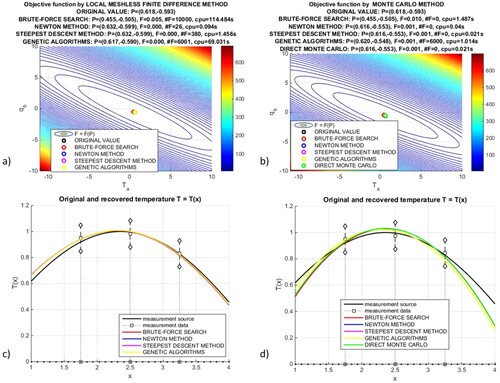
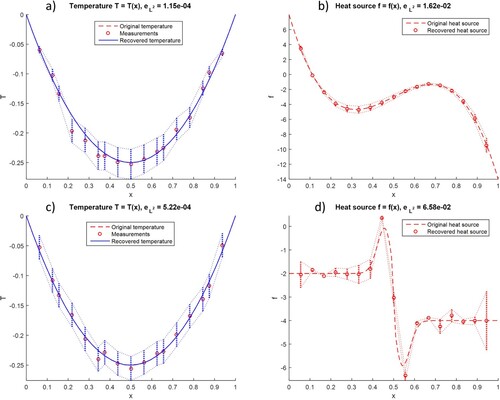
Figure 4. Recovered heat source (a,b) and temperature functions (c,d) of optimization problem with three decision variables and regular mesh, for algorithms combined with FD method (a,c), and algorithms combined with MC method + direct MC method (b,d).

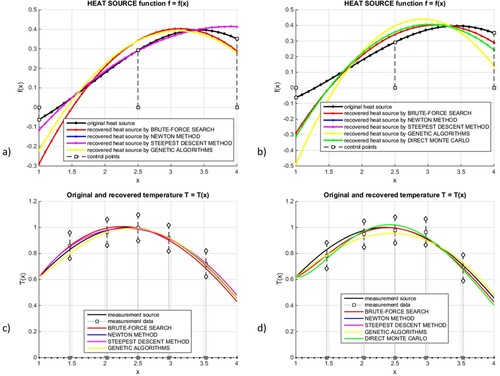
Figure 5. Recovered heat source (a,b) and temperature functions (c,d) of optimization problem with five decision variables and regular mesh, for algorithms combined with FD method (a,c), and algorithms combined with MC method + direct MC method (b,d).

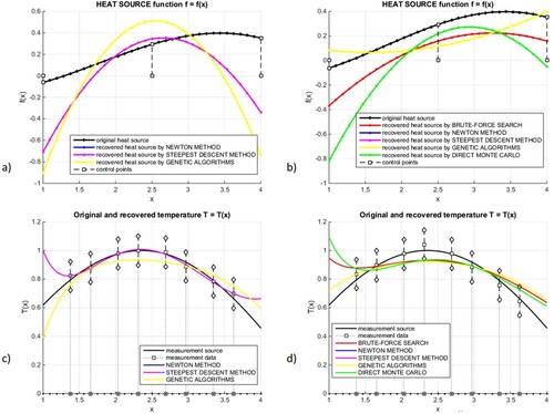
Table 2. Comparison of computational times, required for selected method's combinations for the regular mesh of 33 nodes (i = 1, 2, 3).

number of decision variables	2 ($T_a,q_b$)		3 ($f_i$)		5 ($T_a,q_b,f_i$)
methods' combination	FDM	MC	FDM	MC	FDM	MC
brute search method	114s	1.5s	177s	20s	–	1800s
Newton method	0.02s	0.03s	0.05s	0.03s	0.1s	0.06s
steepest descent method	1.5s	0.02s	1.45s	0.1s	1.4s	0.2s
genetic algorithms	69s	1s	98s	2.5s	145s	4s
direct Monte Carlo method	0.02s		0.03s		0.03s

Numerical experiments, results of which are presented in Figure 6, clearly indicate that the solution convergence, obtained for the set of non-adaptive regular meshes, is much slower than in the case of adaptive clouds of nodes and meshless FDM, regardless of the applied error norm. This phenomena may be explained by the low approximation accuracy in both boundary zones, when using regular mesh and central FD operators. Although regular mesh refinement lowers the global solution error, its extreme values at x = b are not successfully reduced unless local irregular mesh refinement is applied. Therefore, an adaptive cloud with 49 nodes has been generated, which allows to obtain approximately 100 times smaller solution error than in case of a regular mesh with the same number of nodes. Alternatively, to obtain the similar solution error (${10}^{-4}$) using regular meshes, one would have to generate a regular mesh with 1000 nodes. Once the adapted cloud of nodes is generated, computations are performed for all three optimization variants. However, since results for the first (2 decision variables) and the second (3 decision variables) variants do not show any significant differences when compared to those obtained on regular meshes (which are already very precise), results' presentation (including the adaptive distribution of 49 nodes on x-axes) is limited to the third variant (5 decision variable) only (Figure 7). As already shown, this variant exhibited low results accuracy using the regular mesh (Figure 5). Here, a vast improvement of the final results may be observed, as they fit original functions f and T in a more accurate manner. Similarly, comparison of computational times, shown in Table 3, reflects advantages of application of the Monte Carlo algorithm with meshless random walk, either in combination with optimization methods or as the direct approach.

6.4. Selected extensions and applications

In previous chapters, it was assumed that the number of measurement ($m_t$) is small, whereas the unknown heat source function has to be determined on the basis of few degrees of freedom ($m_f$), in order to avoid ill-conditioned and singular (in case $m_f>m_t$) final systems of algebraic equations. Consequently, such computational model may be applied to problems in which temperature T, material λ and heat source f functions are regular, continuous and smooth. However, in case of problems, in which we assume or expect more complex behaviour of T, λ and f, and therefore, we are able to obtain larger number of temperature measurement, the global approximation of the unknown source function (61(61) $\left[\begin{array}{ccc}{\displaystyle \sum _{i=1}^{m_t}{S}_{i,1}^2}& {\displaystyle \sum _{i=1}^{m_t}{S}_{i,1}{S}_{i,2}}& {\displaystyle \sum _{i=1}^{m_t}{S}_{i,1}{S}_{i,3}}\\ {\displaystyle \sum _{i=1}^{m_t}{S}_{i,2}{S}_{i,1}}& {\displaystyle \sum _{i=1}^{m_t}{S}_{i,2}^2}& {\displaystyle \sum _{i=1}^{m_t}{S}_{i,2}{S}_{i,3}}\\ {\displaystyle \sum _{i=1}^{m_t}{S}_{i,3}{S}_{i,1}}& {\displaystyle \sum _{i=1}^{m_t}{S}_{i,3}{S}_{i,2}}& {\displaystyle \sum _{i=1}^{m_t}{S}_{i,3}^2}\end{array}\right]\left[\begin{array}{c}{f}_1\\ f_2\\ f_3\end{array}\right]=\left[\begin{array}{c}{\displaystyle \sum _{i=1}^{m_t}{S}_{i,1}({\hat{T}}_i-m_t{T}_a-s_n{N}_{i,n}{q}_b)}\\ {\displaystyle \sum _{i=1}^{m_t}{S}_{i,2}({\hat{T}}_i-m_t{T}_a-s_n{N}_{i,n}{q}_b)}\\ {\displaystyle \sum _{i=1}^{m_t}{S}_{i,3}({\hat{T}}_i-m_t{T}_a-s_n{N}_{i,n}{q}_b)}\end{array}\right]$(61) ) may be no longer valid. Instead, f may be approximated similarly as T, namely using the regular or irregular mesh of $m_f$ nodes ${\mathbf{x}}_f$ and degrees of freedom $\mathbf{f}=f\left({\mathbf{x}}_f\right)$, independent from $\mathbf{x}$ and $\mathbf{T}$. Moreover, the local low order polynomial approximation of f is required in order to compute its nodal values $f\left(\mathbf{x}\right)$. Although both meshes $\mathbf{x}$ and ${\mathbf{x}}_f$ may be regular, the relevant mapping between them should be constructed, using, for instance, MWLS technique, described in Section 3. Regardless of the applied mapping technique, the mutual relation between $f\left(\mathbf{x}\right)$ and $\mathbf{f}$ degrees of freedom may be denoted as follows (70) $f\left(\mathbf{x}\right)={\mathbf{M}}_f\left(\mathbf{x}\right)\mathbf{f}$(70) where ${\mathbf{M}}_f$ is the $[n\times m_f]$ coefficient matrix. In the simplest (though rather non-realistic) case, where $\mathbf{x}={\mathbf{x}}_f$ and $n=m_f$, ${\mathbf{M}}_f$ is the square identity matrix. The relevant modification of the formula (50(50) $F\left(\mathbf{P}\right)=\sqrt{\frac{1}{m_t}\sum _{i=1}^{m_t}{\displaystyle \frac{1}{\mathrm{\Delta }{T}_i^2}}{(T_a+\frac{1}{N}(\sum _{l=2}^{n-1}{N}_{i,l}{s}_{l}f(x_l,\mathbf{f})+N_{i,n}{s}_n{q}_b)-{\hat{T}}_i)}^2}$(50) ) and the following ones concerns computation of $f(x_l,\mathbf{f})=({\mathbf{M}}_f^{\mathrm{T}}{)}^{〈l〉}\mathbf{f},l=2,\dots ,n-1$. As a consequence, coefficients from ${\mathbf{M}}_f$ appear in the final system of Equation (57(57) $\mathbf{A}\mathbf{P}=\mathbf{B}\left(\hat{\mathbf{T}}\right)$(57) ) instead of values of basis functions ${\mathrm{\Phi }}_j$.

Figure 6. Convergence of the solution error, computed in three norms (global mean $L^2$, maximum $L^{max}$, local $e\left(b\right)$), for the set of (a) regular non-adaptive meshes, (b) irregular adaptive clouds of nodes.

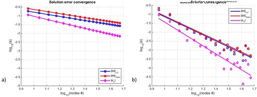
Figure 7. Recovered heat source (a,b) and temperature functions (c,d) of optimization problem with five decision variables and irregular cloud of nodes, for algorithms combined with FD method (a,c), and algorithms combined with MC method + direct MC method (b,d).

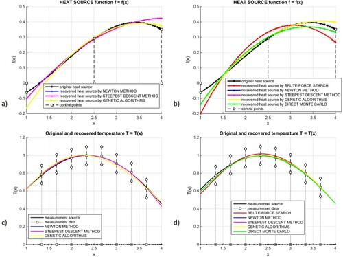
Table 3. Comparison of computational times, required for selected method's combinations for the adaptive cloud with 49 nodes (i = 1, 2, 3).

number of decision variables	2 ($T_a,q_b$)		3 ($f_i$)		5 ($T_a,q_b,f_i$)
methods' combination	MFDM	MC	MFDM	MC	MFDM	MC
brute search method	197s	1.5s	407s	59s	–	4500s
Newton method	0.1s	0.03s	1s	0.09s	2s	0.1s
steepest descent method	1.5s	0.02s	9s	0.4s	13s	0.5s
genetic algorithms	82s	1s	206s	6s	567s	8s
direct Monte Carlo method	0.03s		0.03s		0.03s

Below, results of several benchmark examples are presented, obtained by means of the direct Monte Carlo optimization method only. In all cases, the domain $\mathrm{\Omega }=\left[01\right]$, regular mesh $\mathbf{x}$ with n = 33, $m_t=17$ temperature measurements and $m_f=17$ degrees of freedom of the unknown heat source function are assumed. $N=1000$ random walks are performed in 100 series, with indication numbers properly averaged. Therefore, both deterministic and stochastic errors may be similarly estimated as e<0.03 (i.e. $3\mathrm{\%}$). First, the isotropic material with $\lambda =1$ and analytical solution $T\left(x\right)=\sin \left(2\pi x\right)$, being the source of simulated measurements, are applied. Two types of stochastic measurement noise are provided, namely the noise proportional to temperature (up to $10\mathrm{\%}$ of the original value, $\mathrm{\Delta }{T}_i=0.1T_i$) as well as the constant noise (up to $\mathrm{\Delta }T={0.2}^{\mathrm{o}}\mathrm{C}$). Graphs of the analytical temperature T, measurements $\hat{\mathbf{T}}$ and recovered temperature as well as the original heat source function and its recovered values ${\mathbf{f}}^{\left(\mathrm{o}\mathrm{p}\mathrm{t}\right)}$, with lower ${\mathbf{f}}^{\left(\mathrm{l}\mathrm{o}\mathrm{w}\mathrm{e}\mathrm{r}\right)}$ and upper ${\mathbf{f}}^{\left(\mathrm{u}\mathrm{p}\mathrm{p}\mathrm{e}\mathrm{r}\right)}$ error bounds are presented in Figure 8, for the proportional (Figure 8(a,b)) and constant (Figure 8(c,d)) noise. In graphs' labels mean squared errors (in $L^2$ Euclidean norm) of recovered functions, with respect to the analytical solution, are shown.

The second problem concerns very simple temperature distribution $T\left(x\right)=x(x-1)$, though with material function ascribed by the third-order polynomial $\lambda \left(x\right)=18x^3-27x^2+10x+1$ (yielding positive values for $x\in \left[01\right]$). Results, obtained for the proportional type of measurement noise, are presented in Figure 9(a,b). For the third problem, the continuous material function is replaced by the discontinuous one, whose first derivative may be modelled using the finite representation of the Dirac delta distribution δ, namely (71) $\lambda \left(x\right)=\{\begin{array}{l}1,x\in \left[\begin{array}{cc}0& {\displaystyle \frac{1}{2}}\end{array}\right)\\ 2,x\in \left(\begin{array}{cc}{\displaystyle \frac{1}{2}}& 1\end{array}\right]\end{array},{\displaystyle \frac{\mathrm{d}\lambda }{\mathrm{d}x}}=\delta (x-{\displaystyle \frac{1}{2}})\approx {\displaystyle \frac{2}{h\sqrt{\pi }}}\exp (-{\left({\displaystyle \frac{2x-1}{h}}\right)}^2)$(71) Results, obtained for the constant type of measurement noise $\mathrm{\Delta }T={0.02}^{\mathrm{o}}\mathrm{C}$, are presented in Figure 9(c,d).In each case, a very good agreement may be observed when original and recovered functions are taken into account. It may be surprising to see that heat source function values (primary unknown) are recovered with larger error than the temperature function (secondary unknown). The reason is that ${\mathbf{f}}^{\left(\mathrm{o}\mathrm{p}\mathrm{t}\right)}$ corresponds to pure stochastic solution whereas the final temperature function is obtained from deterministic FD algorithm, which incorporates exactly imposed boundary conditions as well as recovered ${\mathbf{f}}^{\left(\mathrm{o}\mathrm{p}\mathrm{t}\right)}$ values as right-hand sides of a boundary value problem. Furthermore, in case of constant measurement noise, error bounds of f function indicate the largest uncertainty range at borders where the mapping (70(70) $f\left(\mathbf{x}\right)={\mathbf{M}}_f\left(\mathbf{x}\right)\mathbf{f}$(70) ) becomes less accurate.

Figure 8. Recovered heat source (b,d) and temperature functions (a,c) for the isotropic material as well as the measurement noise proportional to temperature values (a,b) and a constant one (c,d).

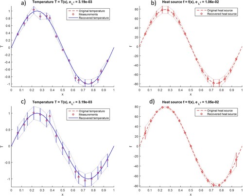
Figure 9. Recovered heat source (b,d) and temperature functions (a,c) for the highly anisotropic (a,b) and heterogeneous (c,d) materials.

Eventually, the inverse transient heat conduction problem is considered. For the sake of simplicity, the isotropic material ($\lambda =const.$) as well as essential boundary conditions are taken into account, whereas temperature $T=T(x,t,\mathbf{f})$ and heat source $f=f(x,t,\mathbf{f})$ functions remain unknown, namely (72) $\{\begin{array}{l}T(a,t,\mathbf{f})=T_a(t,\mathbf{f}),T(b,t,\mathbf{f})=T_b(t,\mathbf{f})\\ \lambda {\displaystyle \frac{{\mathrm{\partial }}^{2}T}{\mathrm{\partial }{x}^2}}-c\rho {\displaystyle \frac{\mathrm{\partial }T}{\mathrm{\partial }t}}=f(x,t,\mathbf{f})\\ T(x,t_0,\mathbf{f})=T_0(x,\mathbf{f})\end{array}$(72) where $t>t_0$, $x\in \left(ab\right)$, $t_0$ is the initial time, c is the specific heat capacity and ρ is the mass density. Let us introduce the regular mesh with n nodes on each kth time level, represented by modules h and $\mathrm{\Delta }t$, respectively. Applying the standard FD schemes to both spatial and time derivatives as well as introducing fixed random walk principles, one obtains probabilities of the next move from the node $(i,k+1)$ located on the unknown time level, namely (73) $p_{i-1,k+1}=p_{i+1,k+1}={\displaystyle \frac{\alpha }{1+2\alpha }},p_{i,k}={\displaystyle \frac{1}{1+2\alpha }}$(73) with possible directions to nearest left $(i-1,k+1)$, right $(i+1,k+1)$ and lower $(i,k)$ nodes, where $\alpha =\frac{\lambda \mathrm{\Delta }t}{c\rho h^2}$ is the Fourier coefficient, corresponding to the unconditionally stable simple implicit time integration scheme. Random walks are performed as long as boundary lines x = a, x = b or the initial time level $t=0$ are reached, which increases the relevant indication numbers of nodes located there. The final Monte Carlo formula, yielding the unknown temperature value $T_{i,k+1}$, is as follows (74) $\begin{array}{rl}{T}_{i,k+1}\left(\mathbf{f}\right)& ={\displaystyle \frac{1}{N}}(\sum _{p=1}^{k+1}(N_{(i,k+1),(1,p)}{T}_a(t_p,\mathbf{f})+N_{(i,k+1),(n,p)}{T}_b(t_p,\mathbf{f}))\\ & +\sum _{j=2}^{n-1}{N}_{(i,k+1),(j,1)}{T}_0(x_j,\mathbf{f})+\sum _{j=2}^{n-1}\sum _{p=2}^{k+1}{N}_{(i,k+1),(j,p)}f(x_j,t_p,\mathbf{f}))\end{array}$(74) Following the analytical differentiation of the objective function based upon the mean squared measurement error between computed (74(74) $\begin{array}{rl}{T}_{i,k+1}\left(\mathbf{f}\right)& ={\displaystyle \frac{1}{N}}(\sum _{p=1}^{k+1}(N_{(i,k+1),(1,p)}{T}_a(t_p,\mathbf{f})+N_{(i,k+1),(n,p)}{T}_b(t_p,\mathbf{f}))\\ & +\sum _{j=2}^{n-1}{N}_{(i,k+1),(j,1)}{T}_0(x_j,\mathbf{f})+\sum _{j=2}^{n-1}\sum _{p=2}^{k+1}{N}_{(i,k+1),(j,p)}f(x_j,t_p,\mathbf{f}))\end{array}$(74) ) and measured ${\hat{T}}_{i,k+1}$ temperatures, according to the direct Monte Carlo optimization method, one obtains the system of algebraic equations and the optimal parameters ${\mathbf{f}}^{\left(\mathrm{o}\mathrm{p}\mathrm{t}\right)}$ for each unknown time level separately, similarly as in (57(57) $\mathbf{A}\mathbf{P}=\mathbf{B}\left(\hat{\mathbf{T}}\right)$(57) ) for the steady heat conduction problem.

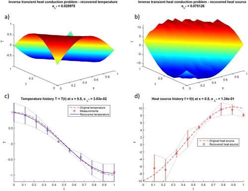
Preliminary results are presented for the benchmark problem with the analytical solution $T(x,t)=\sin (x\pi +t\pi )$, $t_0=0$, n = 33 nodes on each of 10 time levels with $\mathrm{\Delta }t=0.111$ as well as m = 17 measurements on each time level and $m_f=17$ degrees of freedom, representing unknown heat source function. Moreover, non-physical unitary values are assigned to each material parameter λ, ρ and c. Results are presented in Figure 10, namely graphs of recovered temperature and heat source functions in the $(x,t)$ domain (Figure 10(a,b)) as well as their temporal changes for the particular middle node (x = 0.5) along with their corresponding error bounds (Figure 10(c,d)). The measurement noise, proportional to temperature (up to $30\mathrm{\%}$ of the original value), is assumed.

Figure 10. Recovered heat source (b) and temperature functions (a) as well as their histories at x = 0.5 for the benchmark transient heat conduction problem.

7. Final remarks

The inverse thermal problem, formulated as the two-point boundary value problem with unknown temperature function as well as selected unknown load parameters, has been investigated. The primary non-linear optimization problem may be formulated on the basis of additional data namely temperature measurement done at few fixed locations. Regardless of the method of its analysis, multiple solutions of the initial thermal problem are required for the temporarily fixed load parameters. Moreover, optimization algorithms may be computationally demanding (e.g. searching methods) and/or sensitive to the selection of their parameters (e.g. initial solution for gradient methods, admissible load intervals for searching methods).

The numerical model of the thermal problem is based upon the Finite Difference Method, either in a standard (regular meshes of nodes) or meshless variant (arbitrarily irregular clouds of nodes). Despite its simplicity and low computational time, it requires determination of temperature at all nodes. Therefore, the Monte Carlo approach with two types of random walk has been proposed and introduced into both FDM variants. It allows for a stochastic approximation of temperature at measurement locations only, where it is required from the optimization point of view. The novelty of this research includes its application in two different variants, namely as the replacement of the FDM algorithm, or the self-sufficient direct optimization approach. In the first case, it significantly reduces the computational times, although it does not remove drawbacks of the applied optimization method. In the second case, it yields the solution of the inverse problem in a semi-analytical manner, as the solution of small system of linear algebraic equations.

Several numerical benchmark tests with simulated temperature measurements have been executed and their results have been presented and commented in a detailed manner. It has been shown that Monte Carlo-based algorithms are fast and reasonably accurate, though their effectiveness is governed by the proper selection of several parameters, for instance the number of random walks as well as the number and distribution of nodes.

Though obtained results are very encouraging, this research should be considered as the interesting starting point. Inverse thermal problems with multidimensional physical spaces as well as more complex non-stationary heat flows should be taken into consideration. However, the development of the Monte Carlo approach for forward and inverse mechanical problems, with unknown vector (displacements) and tensor (strain, stress) fields, seems to be the most challenging task.

Disclosure statement

No potential conflict of interest was reported by the author(s).

References

- Zienkiewicz OC, Taylor RL. Finite element method its basis and fundamentals. Oxford: Elsevier; 2005.
- Li S, Liu WK. Meshfree and particle methods and their applications. Appl Mech Rev. 2002;55:1–34.
- Liu GR. Mesh free methods: moving beyond the finite element method. Boca Raton (FL): CRC Press; 2003.
- Orkisz J. Finite difference method (part III). In Handbook of computational solid mechanics. Springer-Verlag; 1998. p. 336–431.
- Perrone N, R. Kao N. A general finite difference method for arbitrary meshes. Comput Struct. 1975;5:45–58.
- Liszka T, Orkisz J. The finite difference method at arbitrary irregular grids and its application in applied mechanics. Comput Struct. 1980;11:83–95.
- Milewski S. Selected computational aspects of the meshless finite difference method. Numer Algorithms. 2013;63(1):107–126.
- Wang G, Guo F. A stochastic boundary element method for piezoelectric problems. Eng Anal Bound Elem. 2018;95:248–254.
- Holland JR. Adaptation in natural and artificial systems. Cambridge (MA): MIT Press; 1975.
- Goldberg D. Genetic algorithms in search, optimization and machine learning. Reading (MA): Addison-Wesley Professional; 1989.
- Sabelfeld KK. Monte Carlo methods in boundary value problems. Berlin: Springer-Verlag; 1991.
- Ripley BD. Pattern recognition and neural networks. Cambridge (MA): Cambridge University Press; 2007.
- Moller B, Beer M. Fuzzy randomness, uncertainty in civil engineering and computational mechanics. Berlin: Springer–Verlag; 2004.
- Hansen PC. The L-Curve and its use in the numerical treatment of inverse problems. In: Computational inverse problems in electrocardiology, advances in computational bioengineering. WIT Press; 2000. p. 119–142.
- Cazacu R, Grama L. Steel truss optimization using genetic algorithms and FEA. Procedia Technol. 2014;12(C):339–346.
- Czubacki R, Lewiński T. Topology optimization of spatial continuum structures: made of nonhomogeneous material of cubic symmetry. J Mech Mater Struct. 2015;10(4):519–535.
- Lundgaard C, Sigmund O. Design of segmented off-diagonal thermoelectric generators using topology optimization. Appl Energy. 2019;236:950–960.
- Luh GC, Wu CY. Non-linear system identification using genetic algorithms. Proc Inst Mech Eng Part I J Syst Control Eng. 1999;213(2):105–118.
- Forestier R, Massoni E, Chastel Y. Estimation of constitutive parameters using an inverse method coupled to a 3D finite element software. J Mater Process Technol. 2002;125–126:594–601.
- Kazemi Z, Hematiyan MR, Shiah YC. An efficient load identification for viscoplastic materials by an inverse meshfree analysis. Int J Mech Sci. 2018;136:303–312.
- Attia MH, Fraser S, Osman MOM. On-line estimation of time-variant thermal load applied to machine tool structures using a s-domain inverse solution. Int J Mach Tools Manufact. 1999;39(6):985–1000.
- Jin B, Marin L. The method of fundamental solutions for inverse source problems associated with the steady-state heat conduction. Int J Numer Methods Eng. 2007;69(8):1570–1589.
- Milewski S. Determination of the truss static state by means of the combined FE/GA approach, on the basis of strain and displacement measurements. Inverse Probl Sci Eng. 2019;27(11):1537–1558.
- Mukhopadhyay SC, Ihara I. Sensors and technologies for structural health monitoring: a review, new developments in sensing technology for shm, LNEE 96. Mukhopadhyay SC, editor, Berlin: Springer-Verlag; 2011.
- Hernandez EM. Efficient sensor placement for state estimation in structural dynamics. Mech Syst Signal Process. 2017;85:789–800.
- Helmig T, Al-Sibai F, Kneer R. Estimating sensor number and spacing for inverse calculation of thermal boundary conditions using the conjugate gradient method. Int J Heat Mass Transf. 2020;153:119638.
- Ohe T, Ohnaka K. Boundary element approach for an inverse source problem of the Poisson equation with a one-point-mass like source. Appl Math Model. 1994;18(4):216–223.
- Gu Y, Lei J, Fan CM, et al. The generalized finite difference method for an inverse time-dependent source problem associated with three-dimensional heat equation. Eng Anal Bound Elem. 2018;91:73–81.
- Jiang J, Mohamed SM, Seaid M, et al. Identifying the wavenumber for the inverse Helmholtz problem using an enriched finite element formulation. Comput Methods Appl Mech Eng. 2018;340:615–629.
- Khan MN, Ahmad I, Ahmad H. A radial basis function collocation method for space-dependent inverse heat problems. J Appl Comput Mech. 2020;6:1187–1199.
- Koulouri A, Rimpiläinen V, Brookes M, et al. Compensation of domain modelling errors in the inverse source problem of the Poisson equation: application in electroencephalographic imaging. Appl Numer Math. 2016;106:24–36.
- Rond A, Giryes R, Elad M. Poisson inverse problems by the plug-and-play scheme. J Vis Commun Image Represent. 2016;41:96–108.
- Alves C, Martins N, Roberty N. Full identification of acoustic sources with multiple frequencies and boundary measurements. Inverse Probl Imag. 2009;3(2):275–294.
- Frackowiak A, Wolfersdorf JV, Ciałkowski M. Solution of the inverse heat conduction problem described by the Poisson equation for a cooled gas-turbine blade. Int J Heat Mass Transf. 2011;54(5–6):1236–1243.
- Bergagio M, Li H, Anglart H. An iterative finite-element algorithm for solving two-dimensional nonlinear inverse heat conduction problems. Int J Heat Mass Transf. 2018;126(A):281–292.
- Wen H, Yan G, Chuanzeng Z, et al. The generalized finite difference method for an inverse boundary value problem in three-dimensional thermo-elasticity. Adv Eng Softw. 2019;131:1–11.
- Wang X, Li H, He L, et al. Evaluation of multi-objective inverse heat conduction problem based on particle swarm optimization algorithm, normal distribution and finite element method. Int J Heat Mass Transfer. 2018;127(A):1114–1127.
- Gawad J, Szeliga D. Application of evolutionary algorithms for inverse analysis and computations. Metal Foundry Eng. 2002;28(2):137–150.
- Hafid M, Lacroix M. Inverse method for simultaneously estimating multi-parameters of heat flux and of temperature-dependent thermal conductivities inside melting furnaces. Appl Therm Eng. 2018;14:981–989.
- Mierzwiczak M, Kołodziej JA. The determination of heat sources in two dimensional inverse steady heat problems by means of the method of fundamental solutions. Inverse Probl Sci Eng. 2011;19(6):777–792.
- Wen J, Yamamoto M, Wei T. Simultaneous determination of a time-dependent heat source and the initial temperature in an inverse heat conduction problem. Inverse Probl Sci Eng. 2013;21(3):485–499.
- Nakamura T, Kamimura Y, Igawa H, et al. Inverse analysis for transient thermal load identification and application to aerodynamic heating on atmospheric reentry capsule. Aerosp Sci Technol. 2014;38:48–55.
- Davies AJ, Dixon LCW, Roy R, et al. Regularisation and the inverse problem. Adv Eng Softw. 1999;30(8):557–562.
- Ismailov MI, Çiçek M. Inverse source problem for a time-fractional diffusion equation with nonlocal boundary conditions. Appl Math Model. 2016;40(7):4891–4899.
- Bodin A, Sietsma J, van der Zwaag S. Flow stress prediction during intercritical deformation of a lowcarbon steel with a rule of mixtures and Fe-simulations. Scr Mater. 2001;45(8):875–882.
- Ferreira MDC, Venturini WS. Inverse analysis for two-dimensional structures using the boundary element method. Adv Eng Softw. 2010;41(9):1061–1072.
- Gu Y, Wang L, Chen W, et al. Application of the meshless generalized finite difference method to inverse heat source problems. Int J Heat Mass Transf. 2017;108(Part A):721–729.
- Liu JC, Li XC. Reconstruction algorithms of an inverse source problem for the Helmholtz equation. Numer Algorithms. 2020;84:909–933.
- Metropolis N, Ulam S. The Monte Carlo method. J Am Stat Assoc. 1949;44(247):335–341.
- Eckhardt R, Ulam S, von Neumann J. The Monte Carlo method. Los Alamos Sci. 1987;15:131–137. Special Issue
- Milewski S. Combination of the meshless finite difference approach with the Monte Carlo random walk technique for solution of elliptic problems. Comput Math Appl. 2018;76(4):854–876.
- Mosegaard K, Tarantola A. Monte Carlo sampling of solutions to inverse problems. J Geophys Res. 1995;100(B7):12431–12447.
- Mosegaard K, Sambridge M. Monte Carlo analysis of inverse problems. Inverse Probl. 2002;18(3):R29.
- Hou T, Nuyens D, Roels S, et al. Quasi-Monte Carlo based uncertainty analysis: sampling efficiency and error estimation in engineering applications. Reliab Eng Syst Safety. 2019;19:106549.
- Shen Q, Wu X, Chen J, et al. Solving geosteering inverse problems by stochastic hybrid Monte Carlo method. J Pet Sci Eng. 2018;16:9–16.
- de las Heras MJF, Manguán MC, Millán ER, et al. Determination of SEA loss factors by Monte Carlo filtering. J Sound Vib. 2020;479:115348.
- Pasculli A, Calista M, Sciarra N. Variability of local stress states resulting from the application of Monte Carlo and finite difference methods to the stability study of a selected slope. Eng Geology. 2018;245:370–389.
- Wyatt MJ, Davies G, Snell C. A new difference based finite element method. Instn Engin. 1975;59(2):395–409.
- Lancaster P, Salkauskas K. Surfaces generated by moving least-squares method. Math Comp. 1981;155(37):141–158.
- Lancaster P, Salkauskas K. Curve and surface fitting. London: Academic Press Inc; 1990.
- Milewski S. A Matlab software for approximate solution of 2D elliptic problems by means of the meshless Monte Carlo random walk method. Numer Algorithms. 2020;83(2):565–591.
- Milewski S. Application of the Monte Carlo method with meshless random walk procedure to selected scalar elliptic problems. Arch Mech. 2019;71(4-5):337–375.
- Milewski S. Development of simple effective cloud of nodes and triangular mesh generators for meshless and element-based analyses – implementation in Matlab. Computer Assisted Methods Eng Sci. 2017;24(3):157–180.
- Milewski S, Orkisz J. Improvements in the global a-posteriori error estimation of the FEM and MFDM solutions. Comput Inform. 2011;30(3):639–653.
- Oden JT, Prudhomme S. Goal-oriented error estimation and adaptivity for the finite element method. Comput Math Appl. 2001;41:733–756.
- Jaworska I. On the ill-conditioning in the new higher order multipoint method. Comput Math Appl. 2013;66(3):238–249.
- Milewski S. Meshless finite difference method with higher order approximation – applications in mechanics. Arch Comput Methods Eng. 2012;19(1):1–49.
- Talebi S, Gharehbash K, Jalali HR. Study on random walk and its application to solution of heat conduction equation by Monte Carlo method. Prog Nucl Energy. 2017;96:18–35.
- Reynolds JF. A proof of the random-walk method for solving Laplace's equation in 2-D. Math Gazette Math Assoc. 1965;49(370):416–420.
- Press WH, Teukolsky SA, Vetterling WT, et al. Numerical recipes. Cambridge Univ.Press; 1999. (The art of Parallel Scientific Computing