Unknown polynomial eigenstrains reconstruction with distributed dislocation technique for crack–inclusion interaction

ABSTRACT

The inverse formulation presents mode-I crack–inclusion interaction solution, based on Eshelby’s equivalent inclusion method (EIM) with an unknown filed of induced polynomial eigenstrains (IPE) inside an inclusion, combined with the distributed dislocations technique (DDT) to model the crack face with unknown perturbations in distributed dislocations (PDD). The expression for PDD, determined through Gauss–Chebyshev Quadrature integration of the singular integral equations, is recast in terms of the unknown coefficients of IPE, which form the only set of unknowns. The crack-face boundary condition is exactly satisfied in this step, without solving for the unknowns. The second boundary condition for continuity of stresses at the inclusion boundary is approximately satisfied through discrete-point collocation equations in a subsequent step through the inverse formation. For modest geometric and modulus ratio configurations, the method obtains the perturbed stress intensity factors with reasonable accuracy using only four terms in IPE.

KEYWORDS:

• Continuum dislocations
• inclusions
• equivalent inclusion method
• eigenstrains
• superposition
• inverse problems

1. Introduction

In the presence of matrix cracks, micromechanics analysis of heterogeneous particulate materials is important in many applications, involving an investigation of crack-path trajectory by an inclusion cluster [1–3]. For crack analysis, numerical methods are usually employed, such as finite element method (FEM) [4,5], extended FEM [6], standard boundary element method (BEM) using boundary discretization [7], BEM based on a fundamental solution BEM, which automatically satisfies traction-free condition using crack Green’s function [8–10] and meshless collocation methods [11,12]. Furthermore, a diverse set of solutions are available to capture the elastic interaction field between a crack and inclusion based on numerical and semi-analytical approaches, including (i) boundary integral equation method (BEIM) [13,14]; (ii) Kolosov-Muskhelishvili (K-M) potential equations [15,16]; (iii) using a fundamental solution dislocation-inclusion interaction combined with distributed dislocation technique (DDT) [17–20]; and (iv) Eshelby’s equivalent inclusion method (EIM) [21–29].

In practice, method (i) is most widely used due to its higher accuracy. In contrast, method (ii) is hindered by numerical difficulties due to many coefficients in the expansion of K-M potentials and method (iii) can be used only for simple configurations. The semi-analytical method in (iv) is appealing because of intuitive construct, which can provide additional insight, linearity of eigenstrains, and significantly fewer number of unknowns than BIEM. In addition, eigenstrains are more localized than the elastic field induced by them. The determination of eigenstrains provides the complete elastic field in regions inside and external to the inclusion [30]. The available solutions using Eshelby’s EIM suffer from accuracy since polynomial eigenstrains appear unknowns and require an inverse formulation. For the crack–inclusion interaction field based on inverse-EIM formulation, the elastic field is computed from the contributions due to unknown eigenstrains inside inclusion and the field induced because of perturbations on the crack face. The numerical solution imposes the requirement for satisfaction of the boundary conditions at the crack face and the inclusion boundary. For example, Li and Chen [22] obtained an interaction solution using the perturbation in the stress field of a classical mode-I crack caused by the elastic field due to a transformation eigenstrains inside the inclusion. Shodja et al. [23] and Moschovidis and Mura [24] obtained the interaction field solution by modelling crack and inclusion as elliptic inhomogeneities with unknown polynomial eigenstrains. Wang [21] modelled the inclusion by uniform eigenstrains (UE) and crack by a segment of distributed dislocations. However, the interaction solutions based on the UE are inaccurate, and those using polynomial eigenstrains suffer from numerical instability. Thus, it is a challenge to use Eshelby’s approach for obtaining the crack-inclusion interaction field without sacrificing the accuracy. The paper proposes a new method as an attractive alternative to BIEM by extending the work of Wang [21] and numerically solving for the unknown coefficients of polynomial eigenstrains using collocation.

The direct EIM solution for Eshelby tensor and the elastic field for elliptic inclusions are extended to low-order polynomial eigenstrains [31–33]. For prescribed polynomial eigenstrains in Cartesian coordinates, a remarkable feature is stated as Eshelby’s polynomial conservation, and it implies that a linear eigenstrain shall only induce polynomial elastic field with linear terms without the constant term. A quadratic eigenstrain shall only induce polynomial elastic field with quadratic terms and the constant term without the linear terms for each term in the Eshelby tensor. The interaction problems involving elastic inclusions are based on inverse-EIM formulations, which require reconstructing the unknown polynomial eigenstrains from the available equations of the induced elastic field. In the present work, the inverse formulation satisfies boundary collocation equations for the continuity condition of stresses at the inclusion boundary. Inverse formulations are more complex than a direct problem; and are ill-posed because of the multi-valued nature of an inverse relationship and insufficient or noisy data [34,35]. To alleviate instability in the numerical solution, the development of a general framework for the reconstruction of the unknown polynomial eigenstrains has attracted much attention by Cao et al. [36], Hill [37], Korsunsky et al. [38] and Agrawal [39].

Therefore, the present work focuses on an inverse-EIM-DDT formulation for the crack–inclusion interaction by extending the available solutions for modelling eigenstrains [21–33,36–39], combined with the DDT for modelling crack [11,17–20,40–43]. For illustration, this work considers a mode-I crack interacting with a two-dimensional elastic, isotropic, circular inclusion, perfectly bonded to an isotropic matrix. In the formulation, the inclusion is represented by a sum of the UE and an unknown field of induced polynomial eigenstrains (IPE); and the crack face is represented by a segment of distributed dislocations with unknown density. The perturbation in the distributed dislocations density (PDD) on the crack face caused by the inclusion eigenstrains (UE plus IPE) is obtained from the crack-face tractions by the Gauss–Chebyshev Quadrature formula. In this step, the traction-free crack face boundary condition is satisfied precisely, and the unknown PDD is re-expressed in terms of the unknown coefficients of IPE. Subsequently, the inverse formulation is used to numerically determine the coefficients to satisfy the continuity requirement at the inclusion boundary through discrete-point collocation equations.

The formulation obtains the interaction elastic field solution from the coefficients of IPE as the only unknowns. Within the constraints of non-uniqueness in ill-posed inverse formulation, successive higher-order polynomial eiegnstrains can be added to increase the accuracy of the solution. The paper is organized as follows. The framework for mathematical representation of the inclusion, and the crack is presented in Section 2. Next, the expression for the crack-face tractions and PDD because of the inclusion eigenstrains (UE plus IPE) is obtained in Section 3. Subsequently, in Section 4, the elastic field is dissected into six terms arising from responses of the crack and the inclusion, and superposition solution is obtained for the interaction stress field. The accuracy of the numerical solution is assessed in Section 5. Finally, conclusions are given in Section 6.

2. Background and mathematical preliminaries

2.1. Geometric configuration

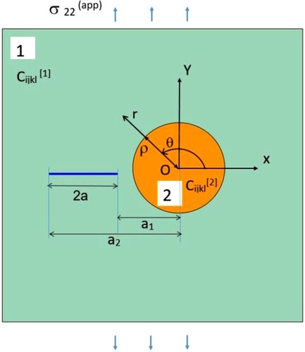
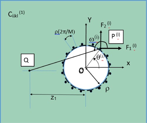
For the crack–inclusion interaction solution, the following geometric configuration is analyzed. A circular inclusion is considered with radius ρ; and interacting matrix crack is assumed to be oriented radially with crack length 2a = (a₂–a₁) and centre-to-centre distance of (a₂ + a₁)/2 from the inclusion centre (Figure 1). In the study, regions 1 and 2 are isotropic and correspond to matrix and inclusion, respectively. Thus, notation is used such that shear modulii are µ₁, µ₂, and Poisson’s ratios are ν_1, ν₂ , for regions 1 and 2, respectively.

Figure 1. Geometric configuration for crack–inclusion interaction.

2.2. Eshelby’s equivalent inclusion method (EIM)

To mathematically represent the stress field inside an inclusion, Eshelby’s EIM replaces inhomogeneous inclusion with homogeneous inclusion plus an equivalent eigenstrain [26,27]. Eigenstrain is a generic term for fictitious stress-free strain inside an inclusion when the surrounding matrix is absent, for example, thermal strain or phase-transformation strain; and eigenstrain is considered zero in the matrix. Due to the inclusion eigenstrain, there is displacement incompatibility at the boundary with the matrix. In the EIM context, when inclusion is bonded to the surrounding matrix to maintain stress and displacement continuity at the inclusion boundary, the induced elastic disturbance inside the inclusion is termed disturbation strain (or stress) field. Based on standard inclusion mechanics for the inclusion region, eigenstrain ε*, elastic strain ε^e, and disturbation strain ε^d are related as follows. (1) $\begin{array}{rl}{\epsilon }_{ij}^d& ={\epsilon }_{ij}^{\ast }+{\epsilon }_{ij}^e\end{array}$(1) (2) $\begin{array}{rl}{\epsilon }_{ij}^{sum}& ={\epsilon }_{ij}^{app}+{\epsilon }_{ij}^d\end{array}$(2) where ${\epsilon }_{ij}^{sum}$ is the total strain field, ${\epsilon }_{ij}^{app}$ is the strain due to applied loads.

2.2.1. EIM solution for the uniform eigenstrains

The most remarkable feature of Eshelby’s EIM states that for an elliptic inclusion in the infinite matrix and subjected to uniformly applied loads, the eigenstrain field is uniform. Hence, the disturbation strain field is also uniform and expressed as follows. (3) ${}^{\{UE\}}{\epsilon }_{ij}^d=S_{ijkl}{}^{\{UE\}}{{\epsilon }_{kl}}^{\ast }$(3) where S_ijkl is the Eshelby tensor and only depends on the material stiffness properties of the matrix and the geometry of the inclusion. Thus, the Eshelby tensor is a constant with respect to spatial coordinates. To specify UE case, left superscript {UE} is used for the notation in Equation (3) and followed in the subsequent text. Thus, based on the definition of Eshelby stress tensor [44], the elastic stresses field inside the circular inclusion is recast as follows. (4) $\left\{\begin{array}{c}{}^{\{UE\}}{\sigma }_{xx}^e\\ {}^{\{UE\}}{\sigma }_{yy}^e\\ {}^{\{UE\}}{\sigma }_{xy}^e\end{array}\right\}=\frac{{\mu }_1}{({\kappa }_1+1)}\left[\begin{array}{ccc}-3& -1& 0\\ -1& -3& 0\\ 0& 0& -1\end{array}\right]\left\{\begin{array}{c}{}^{\{UE\}}{\epsilon }_{xx}^{\ast }\\ {}^{\{UE\}}{\epsilon }_{yy}^{\ast }\\ {}^{\{UE\}}{\epsilon }_{xy}^{\ast }\end{array}\right\}$(4)

2.2.2. Modified EIM for the polynomial eigenstrains

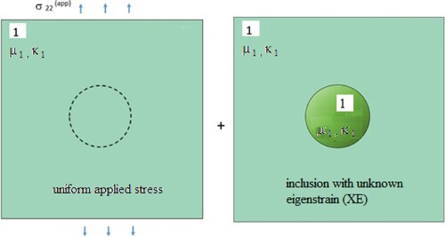
Eshelby’s EIM can be extended to a model elastic field inside an inclusion with unknown non-UE, as shown in Figure 2. Often, the unknown eigenstrains are represented by a polynomial. The general form of polynomial eigenstrains represented in Cartesian coordinates with prescribed coefficients has the following form [31,39] (5a) $\begin{array}{rl}{}^{\{PE\}}{\epsilon }_{xx}^{\ast }& ={}^{\{UE\}}{\epsilon }_{xx}^{\ast }({\alpha }_1[x]+{\alpha }_2[y]+{\alpha }_3[x^2]+{\alpha }_4[xy]+{\alpha }_5[y^2]+\dots )\end{array}$(5a) (5b) $\begin{array}{rl}{}^{\{PE\}}{\epsilon }_{yy}^{\ast }& ={}^{\{UE\}}{\epsilon }_{yy}^{\ast }({\beta }_1[x]+{\beta }_2[y]+{\beta }_3[x^2]+{\beta }_4[xy]+{\beta }_5[y^2]+\dots )\end{array}$(5b) (5c) $\begin{array}{rl}{}^{\{PE\}}{\epsilon }_{xy}^{\ast }& ={}^{\{UE\}}{\epsilon }_{xy}^{\ast }({\delta }_1[x]+{\delta }_2[y]+{\delta }_3[x^2]+{\delta }_4[xy]+{\delta }_5[y^2]+\dots )\end{array}$(5c)

Figure 2. Inclusion with unknown eigenstrains.

Elliptic inclusions with polynomial eigenstrains show special mathematical properties for the induced elastic field [28,29]. Based on Eshelby’s polynomial conservation conjecture, the elastic field inside an elliptic inclusion due to polynomial eigenstrains is composed of polynomial terms of the same degree [29]. Recently, closed-form analytical expressions show that the elements of Eshelby stress tensor have a single linear term for linear eigenstrains; uniform plus quadratic terms for quadratic eigenstrains; and linear plus cubic terms for cubic eigenstrains [31–33,39].

2.2.3. Inverse-EIM for reconstruction of unknown polynomial eigenstrains

The general framework for the inverse problem of eigenstrain reconstruction uses a semi-empirical approach that combines Eshelby’s EIM with data analysis to re-construct components of the unknown eigenstrains. However, often low-degree truncated polynomial series with carefully selected terms is sufficient to simulate the unknown eigenstrains, for example, linear eigensrains [37], quadratic eigenstrains [36,39,45], and cubic eigensrains [46]. Redundant terms in the reconstruction model can lead to undesired fluctuations in the numerical solution [39].

2.3. The distributed dislocation technique (DDT)

2.3.1. Crack model as a continuum of distributed dislocations

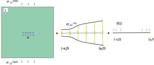
In the continuum analogy, the crack-face displacement discontinuity is mathematically represented by a segment of distributed dislocations. The density of distributed dislocations physically represents the negative slope between the crack faces and becomes infinite at the crack tips [41]. For the crack-face boundary condition of zero traction, the tractions due to distributed dislocations cancel the tractions due to resultant loads on the crack face. The mathematical model of a mode I crack with the unknown density of distributed dislocations is shown in Figure 3.

Figure 3. Representation of a crack with unknown tractions on the crack face: (a) applied uniform stress, (b) unknown tractions on the crack face, (c) unknown distributed dislocations on the crack face (XDD).

2.3.2. Analysis for stress field due to unknown distributed dislocations

In the formulation of crack problems, the distributed dislocation density is unknown and can be obtained from a singular integral equation with a simple Cauchy kernel as given below [17–20,41,42]. (6) $-\frac{({\kappa }_1+1)}{2{\mu }_1}{\sigma }_{22}^{res}(x)=\frac{1}{\pi }{\int }_{-a}^a\frac{B(\xi )}{x-\xi }d\xi -a<x<a$(6) where $x,\xi =0$ is the origin of the coordinate system; Β(ξ) is the density of distributed dislocations, and σ₂₂^res is the resultant normal traction on the crack face under mode I. The resultant traction is the sum of the applied uniform load and the loads because of non-UE inside the inclusion (shown in Section 3). In the integral equation, the traction field is bounded, and the distributed dislocation density is infinite at the crack tips. Furthermore, the distributed dislocation density can be expressed as the product of a fundamental solution and appropriate bounded function as follows [41,47]. (7a) $B(s)=w(s)\phi (s)$(7a) where $s=\xi /a$ is the normalized coordinate between −1and –1 on the crack face, $\phi (s)$ is an unknown bounded function, and $w(s)$ is the fundamental solution. For double singularity at both tips, we have (7b) $w(s)=\frac{1}{\sqrt{1-s^2}}$(7b) Furthermore, using $t=x/a$ as the normalized coordinate on the crack face with values between −1 and –1, and substituting Equations (7a) and (7b), Equation (6) can be recast as follows: (8) $-\frac{({\kappa }_1+1)}{2{\mu }_1}{\sigma }_{22}^{res}(t)=\frac{1}{\pi }{\int }_{-1}^1\frac{1}{\left(\sqrt{1-s^2}\right)}\frac{\phi (s)}{t-s}ds-1<t<1$(8)

2.3.3. Gauss–Chebyshev Quadrature integration formula

Numerical computation of B(s) through Gauss–Chebyshev quadrature converts the singular integral equation (8) into a set of (N−1) algebraic equations with N unknowns using discrete zero points of Chebyshev polynomials as follows [41,47,48]. (9a) $-\frac{({\kappa }_1+1)}{2{\mu }_1}{\sigma }_{22}^{res}(t_k^{(N-1)})=\frac{1}{N}\sum _{j=1}^N\frac{\phi (s_j^N)}{t_k^{(N-1)}-s_j^{(N)}};k=1,2\dots N-1$(9a) where N represents the number of discretization points on the crack face in the interval between −1 and +1; and, $t_k^{(N-1)}=t_1^{(N-1)},t_2^{(N-1)}\dots t_{N-1}^{(N-1)}$ are (N−1) discrete collocation points and the zeros of Chebyshev polynomial of the second kind of order (N−1). Also, $s_j^{(N)}=s_1^{(N)},s_2^{(N)}\dots s_N^{(N)}$ are (N) discrete integration points and the zeros of Chebyshev polynomial of the first kind of order (N).

To solve for N unknowns, the remaining equation is obtained from the requirement of zero crack-face displacements at the crack tips as shown below [41]. (9b) $0=\frac{\pi }{N}\sum _{j=1}^N\frac{\phi (s_j^N)}{1}$(9b) From Equation (9a) and Equation (9b), a numerical solution is obtained for $\phi (s_j^N)$ at N integration points between the two crack tips.

2.3.4. Elastic stress field from distributed dislocations

The matrix stress field (outside the crack), caused by the known distributed dislocations on the crack face, can be numerically obtained by integrating the effects of distributed dislocations at discrete points. Thus, based on standard dislocation mechanics for mode I crack, the stresses in the matrix region at point (χ_x, χ_y) can be computed as follows. (10a) $\begin{array}{rl}{}^{\{\mathrm{\partial }\phi \}}{\sigma }_{yy}({\chi }_x,{\chi }_y)& =\frac{2{\mu }_1}{{\kappa }_1+1}\left(\frac{1}{N}\right)\sum _{j=1}^N{\phi }^{SOL}(s_j)\frac{({\chi }_x/a-s_j)[{({\chi }_x/a-s_j)}^2+3{({\chi }_y/a)}^2]}{{[{({\chi }_x/a-s_j)}^2+{({\chi }_y/a)}^2]}^2}\end{array}$(10a) (10b) $\begin{array}{rl}{}^{\{\mathrm{\partial }\phi \}}{\sigma }_{xx}({\chi }_x,{\chi }_y)& =\frac{2{\mu }_1}{{\kappa }_1+1}\left(\frac{1}{N}\right)\sum _{j=1}^N{\phi }^{SOL}(s_j)\frac{({\chi }_x/a-s_j)[{({\chi }_x/a-s_j)}^2-{({\chi }_y/a)}^2]}{{[{({\chi }_x/a-s_j)}^2+{({\chi }_y/a)}^2]}^2}\end{array}$(10b) (10c) $\begin{array}{rl}{}^{\{\mathrm{\partial }\phi \}}{\sigma }_{xy}({\chi }_x,{\chi }_y)& =\frac{2{\mu }_1}{{\kappa }_1+1}\left(\frac{1}{N}\right)\sum _{j=1}^N{\phi }^{SOL}(s_j)\frac{({\chi }_y/a)[{({\chi }_x/a-s_j)}^2-{({\chi }_y/a)}^2]}{{[{({\chi }_x/a-s_j)}^2+{({\chi }_y/a)}^2]}^2}\end{array}$(10c) where ϕ^SOL (s_j) is obtained at discrete points of Chebyshev zeros on the crack face using Gauss–Chebyshev Quadrature, and coordinates of the point (χ_x, χ_y) are measured with respect to the mid-point of the crack face and lie outside the crack.

3. Perturbations in distributed dislocations caused by unknown eigenstrains

First, the external stress field in the matrix (outside the inclusion) is numerically obtained due to point loads at the inclusion boundary because of the non-uniform unknown eigenstrains, namely, the UE plus an unknown field of IPE. Next, the external stress field is used to determine tractions on the crack face due to the eigenstrains (UE + IPE). Finally, perturbations in distributed dislocations on the crack face caused by the inclusion eigenstrains are numerically obtained using Gauss–Chebyshev Quadrature integration formula.

3.1. Non-UE representation

On account of the interaction with crack, eigenstrains ε_ij* inside inclusion are non-uniform and represented as a sum expressed as given below. (11) ${\epsilon }_{ij}^{\ast }={}^{\{UE\}}{\epsilon }_{ij}^{\ast }+{}^{\{IPE\}}{\epsilon }_{ij}^{\ast },$(11) where ^{UE}ε_ij* is the known UE following Equations (3) and (4). And, ^{IPE}ε_ij* is an unknown field of polynomial eigenstrains, i.e. with unknown coefficients with expressions shown in Equations (5a)–(5c). In the context of the present formulation, these are re-termed as the IPE. The relationship between IPE and the unknown eigenstrains (XE in Figure 2) is shown in the superposition solution (Section 4.2.1).

3.2. Point loads at inclusion boundary due to misfit stresses

In the EIM construct, the eigenstrains can be considered equivalent to surface loads at the inclusion boundary, termed misfit stresses. The misfit stresses depend only on elastic constants of the matrix and the eigenstrains and are expressed as given below [21,27]. (12a) ${\sigma }_{ij}^{\ast m}=2\mu \left[{\epsilon }_{ij}^{\ast }+\left(\frac{\nu }{1-2\nu }\right){\delta }_{ij}{\epsilon }_{kk}^{\ast }\right];k=1,2$(12a) where δ_ij is the Kronecker delta, For numerical computation, the inclusion boundary is discretized into M equal segments with point loads at the centre of each segment. Thus, at each point P⁽ⁱ⁾, i = 1 … M, on the inclusion boundary, discrete-point misfit stresses on each segment are represented as (12b) ${\sigma }_{ij}^{\ast m(i)}=2\mu \left[{\epsilon }_{ij}^{\ast (i)}+\left(\frac{\nu }{1-2\nu }\right){\delta }_{ij}{\epsilon }_{kk}^{\ast (i)}\right];k=1,2$(12b) An approximate solution without considering the unknown IPE was obtained by Wang [21]. However, the misfit stresses exist because of the UE and the unknown IPE, as shown in Figure 4. It is also noted that for uniform remote tension, the shear eigenstrains are zero. Thus, the discrete point loads can be expressed as follows: (13a) $F^{(i)}={}^{\{UE\}}{F}^{(i)}+{}^{\{IPE\}}{F}^{(i)}$(13a) Or, (13b) $F^{(i)}=({}^{\{UE\}}{F}_1^{(i)}+i{}^{\{UE\}}{F}_2^{(i)})+({}^{\{IPE\}}{F}_1^{(i)}+i{}^{\{IPE\}}{F}_2^{(i)})$(13b) Or, (13c) $F^{(i)}=F_1^{(i)}+i{F}_2^{(i)}$(13c) Thus, the contributions from the uniform and the polynomial eigenstrains can be algebraically added at each point. An explicit expression for discretized point loads at M points on inclusion boundary using misfit stresses is given as follows: (14a) $\begin{array}{rl}{F_1}^{(i)}& =\rho \frac{2\pi }{M}[({\sigma }_{11}^{\ast m(i)})\cos {\theta }^{(i)}+({\sigma }_{12}^{\ast m(i)})\sin {\theta }^{(i)}]\end{array}$(14a) (14b) $\begin{array}{rl}{F_2}^{(i)}& =\rho \frac{2\pi }{M}[({\sigma }_{22}^{\ast m(i)})\sin {\theta }^{(i)}+({\sigma }_{12}^{\ast m(i)})\cos {\theta }^{(i)}]\end{array}$(14b) where θ^(ι) i = 1,2 … M is the angle for point P⁽ⁱ⁾ with the x-axis measured counterclockwise.

3.3. Kolosov-Muskhelishvili complex potentials for matrix stresses

The external stress field in the matrix caused due to inclusions eigenstrains is numerically obtained from the cumulative contribution of the discretized point loads (Figures 4 and 5) through K-M potentials [49,50]. For the origin O selected as in Figure 5, the complex coordinate for point P⁽ⁱ⁾ on the inclusion boundary is expressed as (15) ${\upsilon }^{(i)}=\rho (\cos {\theta }^{(i)}+i\sin {\theta }^{(i)})$(15) Furthermore, let point Q has a complex coordinate z. The K-M potentials for stress field at point Q due to complex point load at a point P⁽ⁱ⁾ given by $F_1^{(i)}+i{F}_2^{(i)}$ are expressed as follows [21,49] (16a) $\begin{array}{rl}{\mathrm{\Gamma }}^{(i)}(z)& =-\frac{F{{}_1^{(i)}}_1+i{F}_2^{(i)}}{2\pi (1+{\kappa }_1)}\frac{1}{(z-{\upsilon }^{(i)})}\end{array}$(16a) (16b) $\begin{array}{rl}{\mathrm{\Psi }}^{(i)}(z)& =\frac{\kappa (F_1^{(i)}-i{F}_2^{(i)})}{2\pi (1+{\kappa }_1)}\frac{1}{(z-{\upsilon }^{(i)})}\end{array}$(16b) where κ is the Kolosov parameter for plain strain givenby ${\kappa }_1=3-4{\nu }_1$. Thus, K-M complex potentials to compute the stress field at Q due to point loads at P⁽ⁱ⁾ for i = 1,2 … M are expressed as given below. (17a) $\begin{array}{rl}\mathrm{\Gamma }(z)& =\sum _{i=1}^M{\mathrm{\Gamma }}^{(i)}(z)\end{array}$(17a) (17b) $\begin{array}{rl}\mathrm{\Psi }(z)& =\sum _{i=1}^M{\mathrm{\Psi }}^{(i)}(z)\end{array}$(17b) Using the above complex potentials, complex stress field in the matrix region caused by inclusion eigenstrains is obtained from the standard K-M equations as follows: (18a) $\begin{array}{rl}{\sigma }_{11}+{\sigma }_{22}& =2\left[\mathrm{\Gamma }(z)+\stackrel{-}{\mathrm{\Gamma }}(z)\right]\end{array}$(18a) (18b) $\begin{array}{rl}{\sigma }_{22}-{\sigma }_{11}+2i{\sigma }_{12}& =2\left[\stackrel{\mathrm{\_}}{z}{\mathrm{\Gamma }}^{\mathrm{\prime }}(z)+\mathrm{\Psi }(z)\right]\end{array}$(18b) where overbar denotes complex conjugate and superscript ′ denotes the derivative of the K-M potentials.

Figure 4. Point loads due to misfit stress because of eigenstarins for a segment.

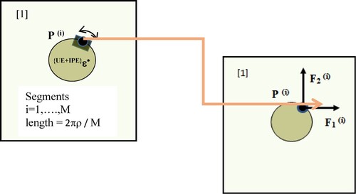
Figure 5. Computation of matrix stress field using discrete points loads on the inclusion boundary.

3.4. Tractions on the crack face

To compute crack-face tractions points Q^(k), k = 1, N−1 are selected on the crack face with origin O represented as z^(k). Thus, using Equation (15), the complex distance PQ (Figure 5) is re-expressed as given below. (19) $z^{(k)}-{\upsilon }^{(i)}=d^{(i,k)}[\cos {\omega }^{(i,k)}+i\sin {\omega }^{(i,k)}]$(19) where ${\omega }^{(i,k)}$ is the angle between QP and x-axis, and d is real and represents the modulus of PQ. Furthermore, k’s are selected as the zeros of Chebyshev polynomials of the second kind, in agreement with equation (9a). Thus, substituting the above equations, namely, (16a), (16b), (17a), (17b) and (19), with the algebraic arrangement, the stresses from K-M equations given by Equations (18a) and (18b) can be recast for the relevant traction component as given below. (20) ${}^{\{UE+IPE\}}{\sigma }_{22}(z^{(k)})=\frac{1}{2\pi (1+{\kappa }_1)}\sum _{i=1}^M\frac{1}{d^{(i,k)}}\left\{\begin{array}{c}(F_2^{(i)})\sin {\omega }^{(i,k)}[(-3-{\kappa }_1)+4{\cos }^2{\omega }^{(i,k)}]+\\ ({F_1}^{(i)})\cos {\omega }^{(i,k)}[(-1+{\kappa }_1)-4{\sin }^2{\omega }^{(i,k)}]\end{array}\right\}$(20) The summation in Equation (20) is for the stress field due to point loads at each P⁽ⁱ⁾’s, which can be linearly added. Also, the tractions computed in Equation (20) are based on F₁⁽ⁱ⁾ and F₂ ⁽ⁱ⁾ at each discrete point P⁽ⁱ⁾ and contain contributions corresponding to each eigenstrain term (UE + IPE) in Equation (13a)–(13c). Because of linearity, the contributions can be algebraically added from each eigenstrain term. The unknown coefficients of IPE corresponding to each discrete point loads F₁⁽ⁱ⁾ and F₂ ⁽ⁱ⁾ given are expressed explicitly by a column vector, shown in Appendix 1.

3.5. Perturbations in distributed dislocations on the crack face

In Equation (20), the crack-face tractions are obtained at points Q^(k), k = 1, N−1 with coordinates z^(k), selected as the zeros of Chebyshev polynomial of the second kind (Section 2.3.3). After this, distributed dislocations on the crack face are computed at discrete points R^(τ), τ = 1, N with coordinates ζ^(τ) that are the zeros of Chebyshev polynomial of the first kind using Gauss–Chebyshev Quadrature formula shown in Equation (9a). The distributed dislocations represent the perturbations caused by the eigenstrains (UE + IPE) and are termed PDD. The relationship between PDD and unknown distributed dislocation (XDD) is shown in Section 4.2.2.

Thus, the PDD cancels the resultant crack-face tractions obtained in Equation (20), corresponding to each contribution on account of terms corresponding to the UE the unknown IPE. Similar to the tractions, the distributed dislocations at each R^(τ), τ = 1, N can also be algebraically added because of the linearity of contributions from each polynomial eigenstrain term. Thus, PDD on the crack face caused by the elastic interaction with inclusion eigenstrains can be expressed as follows. (21) ${}^{\{PDD\}}\phi ({\zeta }^{(\tau )})={}^{\{UE\}}\phi ({\zeta }^{(\tau )})+{}^{\{IPE\}}\phi ({\zeta }^{\tau })$(21) The first term in Equation (21) can be expressed as follows. (22a) ${}^{\{UE\}}\phi ({\zeta }^{(\tau )})=({}^{\{UE\}}{\epsilon }_{xx}^{\ast })[{\phi }_1({\zeta }^{(\tau )})]+({}^{\{UE\}}{\epsilon }_{yy}^{\ast })[{\phi }_2({\zeta }^{(\tau )})]+({}^{\{UE\}}\epsilon {}_{xy}^{\ast })[{\phi }_3({\zeta }^{(\tau )})]$(22a) Furthermore, the second term in Equation (21) corresponding to contribution from IPE can be expanded explicitly involving 3Π unknown coefficients of IPE as follows. (22b) ${}^{\{IPE\}}\phi ({\zeta }^{(\tau )})=\sum _{p=1}^{\mathrm{\Pi }}\left(\begin{array}{ccccc}({\alpha }_p)[{}_p^{\{\alpha \}}\phi ({\zeta }^{(\tau )})]& +& ({\beta }_p)[{}_p^{\{\beta \}}\phi ({\zeta }^{(\tau )})]& +& ({\gamma }_p)[{}_p^{\{\gamma \}}\phi ({\zeta }^{(\tau )})]\end{array}\right)$(22b) where α_p, β_p and γ_p are the unknown coefficients of IPE for p = 1, … Π, and expressed as a column vector, ^{IPE}Θ in Appendix 1. The quantities associated with each term at point R with coordinates ζ^(τ) are completely determined by Gauss–Chebyshev Quadrature. Thus, a crack analysis is performed using numerical Green’s function determination, like meshless solutions [10,11]. Appendix 2 is used to re-express Equation (22b), as shown in Section 4.4.

4. Superposition solution for crack–inclusion interaction

4.1. An overview of the computation strategy

The present crack–inclusion interaction solution is based on a semi-analytical approach and uses inverse-EIM formulation to model the inclusion and the DDT model for the crack. The interaction stress field is obtained by the superposition of the stress field of the classical crack, stress field of the classical inclusion, and two perturbation fields due to the effect of elastic interaction between two. The perturbation numerically satisfies the boundary condition requirements at the crack face and the inclusion boundary. In the computation strategy suggested in this work, the perturbation stress field is obtained such that the perturbation on inclusion is represented by IPE based on the unknown coefficients of the IPE. The combined perturbation on the crack face termed perturbation in distributed dislocations (PDD), is induced by the UE and IPE. As shown in Section 3.5, the coefficients of the polynomial eigenstrains also form the unknowns in the computation of PDD.

In the superposition solution, the crack-face boundary condition is satisfied in a prior step (Section 4.4), without solving the unknown coefficients. The subsequent step solves the unknown coefficients to satisfy the continuity condition at the inclusion boundary through collocation (Sections 4.5 and 4.6).

4.2. Scheme to dissect the elastic fields

The formulation uses the solutions for two auxiliary problems combined to obtain the interaction stress field for the problem shown in Figure 1. The first is the elastic field response inside the inclusion and surrounding matrix, expressed by an unknown field of eigenstrains (XE), as shown in Figure 2. The second is the elastic field response on the crack face and surrounding matrix, expressed by the unknown density of distributed dislocations (XDD), as shown in Figure 3. The relationship between XE and IPE is obtained in Section 4.2.1. Also, the relationship between XDD and PDD is obtained in Section 4.2.2.

4.2.1 Response of elastic interaction inside the inclusion and surrounding matrix

In the absence of crack, based on Eshelby’s standard EIM, an elliptic inclusion in an infinite matrix subjected to uniform remote stress experiences UE. The unknown non-uniform eigenstrain, denoted by XE (Figure 2) captures the interaction effect due to the crack and can be decomposed as the sum of the known uniform part (UE) and an unknown non-uniform part (YE) as follows. (23a) $\text{XE = UE + YE}$(23a) Furthermore, YE can be decomposed as follows. (23b) $\text{YE = NE + IPE}$(23b) where an elastic field outside the inclusion caused by NE is that of a classical crack, and IPE is an unknown polynomial eigenstrain inside the inclusion. The present formulation identifies NE as a nascent (non-uniform, fictitious) eigenstrain, which is the first approximation of YE, and is not caused by elastic interaction with the crack. The external field caused by NE is the same for all inclusion modulus ratios. Thus, the elastic field induced by NE is known. Furthermore, the elastic field inside the inclusion because of IPE can be obtained analytically for low-degree polynomial eigenstrains [26–28] in terms of the unknown polynomial coefficients of IPE. The elastic field in the surrounding matrix due to IPE is obtained numerically in Section 3.3.

4.2.2. Elastic interaction response on the crack face and surrounding matrix

Based on the DDT model in the absence of inclusion, a classical mode I crack in an infinite matrix under uniform remote stress can be modelled by a known density of distributed dislocations corresponding to the uniform crack-face traction, termed KD. In the presence of inclusion, the unknown distributed dislocations are denoted XDD (Figure 3), and the effect of elastic interaction is captured due to the inclusion because of UE and IPE. Thus, XDD can be decomposed as the sum of known distributed dislocations (KD) and unknown perturbation in distributed dislocations (PDD) caused by the elastic interaction with the inclusion, as follows. (24a) $\text{XDD = KD + PDD}$(24a) Furthermore, PDD is decomposed as follows. (24b) $\text{PDD = UDD + IPDD}$(24b) where UDD and IPDD correspond to perturbation in the density of distributed dislocation caused respectively by point-loads [F₁^{U}(i)+ iF₂^{U}(i) ] because of the known UE, and point-loads [F₁^{IPE}(i) + iF₂^{IPE}(i) ] because of the unknown IPE. The expressions for PDD are derived in Section 3.5. Thus, UDD and IPDD are synonymous with UE and IPE, respectively, for computation of the unknown distributed dislocations.

4.3. Computation of the interaction stress field

From graphical illustrations (Figures 2 and 3), the interaction problem in Figure 1 reduces to homogeneous matrix material subjected to eigenstrains (XE) in the inclusion region and distributed dislocations (XDD) on the crack face, where boundary conditions need to be satisfied on the crack face and at the inclusion boundary. Thus, using Equations (23a) and (23b), the interaction field for the inclusion and surrounding matrix region can be expressed as follows. (25a) ${}^{inclusion}{\sigma }_{ij}^{SOL}={\sigma }_{ij}^{app}+{}^{\{UE\}}{\sigma }_{ij}^e+{}^{\{NE\}}{\sigma }_{ij}^e+{}^{\{IPE\}}{\sigma }_{ij}^e$(25a) where ^{UE}σ_ij^e represents the elastic stress field caused by UE, and other terms represent elastic stress field indicated by the corresponding left superscripts, and the coefficients of IPE are unknowns. Similarly, using Equations (24a) and (24b), the interaction field for the outside of the crack face in the surrounding matrix region can be expressed as follows. (25b) ${}^{crack}{\sigma }_{ij}^{SOL}={\sigma }_{ij}^{app}+{}^{\{KD\}}{\sigma }_{ij}^{\mathrm{\partial }\phi }+{}^{\{UDD\}}{\sigma }_{ij}^{\mathrm{\partial }\phi }+{}^{\{IPDD\}}{\sigma }_{ij}^{\mathrm{\partial }\phi }$(25b) where ^{KD}σ_ij^ϕ represents the elastic stress field caused by known distributed dislocations (KD), and other terms represent elastic stress fields indicated by the corresponding left superscripts.

Thus, using Equations (25a) and (25b), the interaction field in the matrix region comprises the effect of six components UE, NE, IPE, KD, UDD, and IPDD. Based on the definition of NE in Section 4.2.1, the elastic stress field outside the inclusion and surrounding matrix is the elastic field of the classical crack, caused by KD, i.e. expressed in mode I stress intensity factor K_I. The elastic stress field inside the inclusion and surrounding matrix because of IPE is obtained from K-M potential equations based on the unknown coefficients of IPE in Section 3. Furthermore, based on the observation in Section 4.2.2, distributed dislocations UDD and IPDD can be numerically computed, respectively, from eigenstrains UE and IPE. Therefore, the interaction stress field for the matrix region surrounding the crack, outside the crack face, and excluding the inclusion region, can be obtained by adding the contributions, as follows. (26) ${\sigma }_{ij}^{SOL}={\sigma }_{ij}^{app}+\frac{K_I^{}}{\sqrt{2\pi r}}+{}^{\{UE\}}{\sigma }_{ij}^e+{}^{\{IPE\}}{\sigma }_{ij}^e+{}^{\{UDD\}}{\sigma }_{ij}^{\mathrm{\partial }\phi }+{}^{\{IPDD\}}{\sigma }_{ij}^{\mathrm{\partial }\phi }$(26) where the second term represents the solution of a classical crack (without inclusion) under the applied uniform remote stress, and the third term represents the solution of classical inclusion (without crack) under applied uniform remote stress. Next, the fourth term represents the elastic stress field based on unknown coefficients of IPE. Next, the fifth and sixth terms are numerically computed using Gauss–Chebyshev Quadrature in Section 3.5, and the fifth term is based on known perturbations UDD, and the sixth term is based on unknown perturbations IPDD. Thus, the fourth and sixth terms contain the unknowns, which are the unknown coefficients of IPE (Appendix 2).

4.4. Crack face boundary condition: step one

Mathematically, the boundary condition of traction-free crack face for mode I crack implies (Figure 1) (27) ${\sigma }_{22}^{SOL}(x;y=0)=0-a_1\le x\le -a_2$(27) In the interaction stress field solution given by Equation (26), the crack-face boundary condition is already satisfied in the formulation through expression for the distributed dislocations (Section 3.5). The numerical computation serendipitously performs a key operation to enable the present EIM-DDT formulation by achieving variable-separable since Equation (22b) re-constructs the expression for the unknown distributed dislocations in terms of the unknown coefficients of IPE. Using vector notation in Appendices 1 and 2, the expressions for UDD and IPDD in Equations (22a) and (22b) can be given as follows: (28a) $\begin{array}{rl}UDD& ={}^{\{UE\}}\phi ({\zeta }^{(\tau )})=\{{}^{\{UE\}}{G}_1{}^{(\tau )}{\}}_{1x3}\{{}^{\{UE\}}{\epsilon }^{\ast }{\}}^{T}3x1\end{array}$(28a) (28b) $\begin{array}{rl}IPDD& ={}^{\{IPE\}}\phi ({\zeta }^{(\tau )})=\{{}^{\{IPE\}}{G}_2{}^{(\tau )}{\}}_{1x3\mathrm{\Pi }}\{{}^{\{IPE\}}\mathrm{\Theta }{\}}_{3\mathrm{\Pi }x1}\end{array}$(28b) where vectors ^{UE}G₁^(τ), ^{IPE}G₂ ^(τ) are given in Appendix 2. The vectors ^{UE}ε* and ^{IPE}Θ are given in Appendix 1. Furthermore, ^{UE}G₁^(τ) and ^{IPE}G₂ ^(τ) are row vectors of size 3 × 1, and 3Π×1, respectively, and their elements include contributions from all polynomial eigenstrain terms, corresponding to index p, p = 1 … Π.

4.5. Continuity condition at the inclusion boundary: step two

4.5.1. Stress continuity equation at the inclusion boundary

The requirement for continuity of stresses at inclusion boundary is approximately satisfied through collocation, without imposing displacement continuity. The collocation procedure computes the unknown coefficients of IPE, expressed by the vector ^{IPE}Θ by the requirement of continuity of radial and circumferential shear stresses. Mathematically, the continuity at the inclusion boundary implies the following. (29a) $\begin{array}{rl}{}^{[2]}{\sigma }_{rr}^{SOL}(\rho \cos \theta ,\rho \sin \theta )& ={}^{[1]}{\sigma }_{rr}^{SOL}(\rho \cos \theta ,\rho \sin \theta ),0\le \theta \le 2\pi \end{array}$(29a) (29b) $\begin{array}{rl}{}^{[2]}{\sigma }_{r\theta }^{SOL}(\rho \cos \theta ,\rho \sin \theta )& ={}^{[1]}{\sigma }_{r\theta }^{SOL}(\rho \cos \theta ,\rho \sin \theta ),0\le \theta \le 2\pi \end{array}$(29b) Furthermore, the interaction field solution in Equation (26) has first, second, and third terms with known stress fields of classical type, and each term unconditionally satisfies the stress continuity requirement at the inclusion boundary. Thus, normal and shear components of stresses in the fourth term are required to match with those in the fifth and sixth terms at the inclusion boundary as follows. (30) ${}^{\{UDD\}}{\sigma }_{ij}^{\mathrm{\partial }\phi }+{}^{\{IPDD\}}{\sigma }_{ij}^{\mathrm{\partial }\phi }={}^{\{IPE\}}{\sigma }_{ij}^e;ij=rr,r\theta r=\rho ,0\le \theta \le 2\pi$(30) where based on the configuration in Figure 1, the left-hand side represents the interaction stress field at the inclusion boundary in the matrix region due to perturbations in the density of distributed dislocations, namely, UDD (synonymous with UE in Equation (28a)) and IPDD (synonymous with IPE in Equation (28b)). The right-hand side represents the interaction stress field at the inclusion boundary due to IPE. Thus, Equation (30) can be re-expressed as follows: (31) ${}^{\{UE\}}{\sigma }_{ij}^{\mathrm{\partial }\phi }+{}^{\{IPE\}}{\sigma }_{ij}^{\mathrm{\partial }\phi }={}^{\{IPE\}}{\sigma }_{ij}^e;ij=rr,r\theta r=\rho ,0\le \theta \le 2\pi$(31)

4.5.2. Discrete-point collocation equations

The collocations points for the interaction problems are preferred on the boundary [51,52]. However, the analytical solution of the Eshelby tensor is available only for low-order polynomials. Thus, the right-hand side in Equation (31) is numerically computed at a discrete set of L collocation points, which are selected close to the inclusion boundary and not on the boundary (Figures 6 and 7), as follows: (32a) $\begin{array}{rl}{\eta }_x^{(i)}& =x({\eta }^{(i)}),i=1,2\dots L\end{array}$(32a) (32b) $\begin{array}{rl}{\eta }_y^{(i)}& =y({\eta }^{{}_{(i)}});⋮i=1,2\dots L\end{array}$(32b) Thus, using Equations (32a) and (32b), the right-hand side in equation (31) is expressed at discrete points as follows: (33a) ${}^{\{IPE\}}{\sigma }_{ij}^e({\eta }_{(x)}^{(i)},{\eta }_y^{(i)})={[\mathrm{\Psi }(\eta {}_x^{(i)},{\eta }_y^{(i)}){]}_{}}_{3x3\mathrm{\Pi }}\{{}^{\{IPE\}}\mathrm{\Theta }{\}}_{3\mathrm{\Pi }x1};$(33a) where stress field σ_ij represents the three Cartesian stress components, namely, σ_xx, σ_yy, σ_xy at each collocation grid point and Ψ, with dimension 3 × 3Π , is numerically obtained based on polynomial eigenstrains with the unknown coefficients, using the procedure shown in Section 3.3.

Figure 6. Sketch for collocation grid.

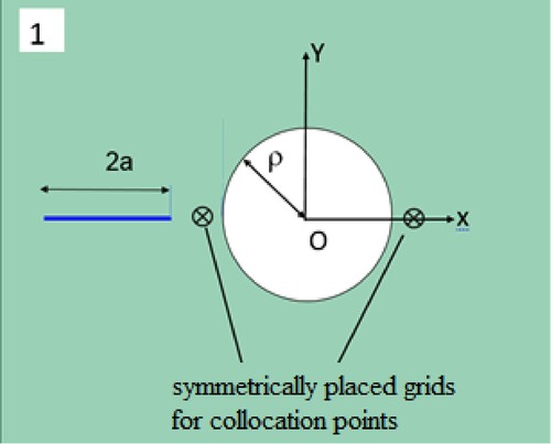
Figure 7. Gridpoint for collocation equations.

Furthermore, using the expression for perturbation in the density of distributed dislocations, UDD and IPDD, in Equations (28a) and (28b) respectively, the matrix stress field caused by distributed dislocations can be numerically obtained from Equations (10a)–(10c). Thus, using Equations (32a) and (32b), terms on the left-hand side in Equation (31) are expressed at discrete points as follows. (33b) $\begin{array}{rl}{}^{\{UE\}}{\sigma }_{ij}^{\mathrm{\partial }\phi }({\eta }_x^{(i)},{\eta }_y^{(i)})& =[{}^{\{UE\}}{H}_1({\eta }_x^{(i)},{\eta }_y^{(i)}){]}_{3x3}\{{}^{\{UE\}}{\epsilon }^{\ast }{\}}_{3x1};\end{array}$(33b) (33c) $\begin{array}{rl}{}^{\{IPE\}}{\sigma }_{ij}^{\mathrm{\partial }\phi }({\eta }_x^{(i)},{\eta }_y^{(i)})& =[{}^{\{IPE\}}{H}_2(\eta {}_x^{(i)},{\eta }_y^{(i)}){]}_{3x3\mathrm{\Pi }}\{{}^{\{IPE\}}\mathrm{\Theta }{\}}_{3\mathrm{\Pi }x1};\end{array}$(33c) where ^{UE}H₁ and ^{IPE}H₂ have dimensions 3 × 3 and 3 × 3Π, respectively, and obtained from, ^{UE}G₁^(τ) and ^{IPE}G₂ ^(τ), respectively.

4.6. Optimization solution for the unknown coefficients of IPE

Collocation involves polar coordinate equations for the stresses at discrete collocation points (η₁ … η_L) to satisfy the requirement for inclusion boundary continuity approximately. Thus, through coordinate transformation and substituting Cartesian component expressions for each stress term from Equations (33a)–(33c) into equation (31), the following equations are obtained for the radial and tangential shear components at each collocation point [46]. (34a) $\begin{array}{rl}\left[\begin{array}{c}{\mathrm{\Lambda }}_{rr}\\ {\mathrm{\Lambda }}_{r\theta }\end{array}\right]{}^{\{UE\}}{H}_1({\eta }_x^{(i)},{\eta }_y^{(i)}{)}_{3x3}\{{}^{\{UE\}}{\epsilon }^{\ast }\}& =\left[\begin{array}{c}{\mathrm{\Lambda }}_{rr}\\ {\mathrm{\Lambda }}_{r\theta }\end{array}\right][\mathrm{\Psi }({\eta }_x^{(i)},{\eta }_y^{(i)})-{}^{\{IPE\}}{H}_2({\eta }_x^{(i)},{\eta }_y^{(i)})]\{{}^{\{IPE\}}\mathrm{\Theta }\}\end{array}$(34a) (34b) $\begin{array}{rl}\left\{\begin{array}{c}{\sigma }_{rr}({\eta }_x^{(i)},{\eta }_y^{(i)})\\ {\sigma }_{r\theta }({\eta }_x^{(i)},{\eta }_y^{(i)})\end{array}\right\}& ={\left[\begin{array}{c}{\mathrm{\Lambda }}_{rr}\\ {\mathrm{\Lambda }}_{r\theta }\end{array}\right]}_{2x3}{\left\{\begin{array}{c}{\sigma }_{xx}({\eta }_x^{(i)},{\eta }_y^{(i)})\\ {\sigma }_{yy}({\eta }_x^{(i)},{\eta }_y^{(i)})\\ {\sigma }_{xy}({\eta }_x^{(i)},{\eta }_y^{(i)})\end{array}\right\}}_{3x1}\end{array}$(34b) For an over-determined system in Equation (34a) with 3Π unknowns, having total collocation points denoted as L, the number of equations is 2L such that 2L > 3Π. The equation system can be solved using least square residue error minimization through MATLAB [53]. Alternatively, to improve numerical stability backward substitution method can be used in inverse formulation solution [54].

5. Numerical examples

5.1. Illustration of equations for computation of the unknowns

Benchmark examples by Erdogan et al. [18] and Rooke and Cartwright [55] obtain the perturbed stress intensity factor with parametric variation of inclusion radius, clear separation distance and inclusion modulus ratios. The present method obtains a numerical solution within the constraints of inverse reconstruction of the unknown eigenstrains. The salient features of the computation are detailed in this section. An accuracy assessment of the results is shown in Sections 5.2 and 5.3 by numerical examples.

5.1.1. Numerical parameters

For all selections of geometric and material parameters, the numerical computation for interaction solution involves three numerical parameters: M, discretization points for point loads on the inclusion boundary; N, discretization points for Gauss–Chebyshev Quadrature integration on the crack face; and L, collocation points for discrete-point continuity equations on the inclusion boundary. The numerical solution selects M = 300, N = 20 and L = 36 and has good stability concerning all the numerical parameters.

5.1.2. Representation of the unknown IPE

Inverse problems seek an underlying quantitative relationship to estimate input quantities from available discrete data of output quantity. Eigenstrain reconstruction is a classical inverse boundary value interaction problem, whereas, forward EIM obtains the elastic field from prescribed eigenstrains.

Mathematically, the conditions for well-posedness are the existence, uniqueness, and stability of the numerical solution [34,35]. Thus, an inverse eigenstrain reconstruction formulation is ill-posed on account multi-valued nature of an inverse relationship and insufficient data and requires a numerical solution. By expanding the work of Hill [37] for linear eigenstrains reconstruction, the general framework for polynomial eigenstrains [36–39] provides guidelines for the pruning procedure of the optimization cost function. Furthermore, redundant terms can be pruned based on the implications of the polynomial conservation conjecture [39]. The guidelines suggest the selection of the unknowns to avoid redundant terms and satisfy the following:

• select appropriate eigenstrain components and omit some eigenstrain components that do not affect the elastic field,such as shear eigenstrains; select reasonable distribution for each eigenstrain component, avoiding redundant terms. For example, avoid odd-powered terms in reconstructing even-powered eigenstrains and vice versa.

In Equation (34), coefficients of IPE form the only unknowns. Using the guidelines [36,39] IPE are represented by truncated polynomial series with unknown coefficients as follows. (35a) $\begin{array}{rl}{}^{\{IPE\}}{\epsilon }_{xx}^{\ast }& ={}^{\{U\}}{\epsilon }_{xx}^{\ast }\{{\alpha }_0+{\alpha }_1(x)+{\alpha }_6(x^3)-{\alpha }_8(x{y}^2)+\dots \}\end{array}$(35a) (35b) $\begin{array}{rl}{}^{\{IPE\}}{\epsilon }_{yy}^{\ast }& ={}^{\{U\}}{\epsilon }^{\ast }\{{\beta }_0+{\beta }_1(x)+{\beta }_6(x^3)-{\beta }_8(x{y}^2)+\dots \}\end{array}$(35b) where IPE is assumed to have only the normal eigenstrains with α_i = β_i for all i to reduce the computation. Therefore, only four terms are used without shear components in the formulation, which are adequate for moderate geometric configurations (Sections 5.2 and 5.3).

5.1.3. Approximations in numerical solution of IPE using collocation

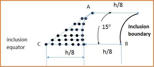
The collocation equations rely on the stresses at the boundary of the inclusion available from the Eshelby stress tensor solution. However, the Eshelby tensor solution is available in an analytical form for only low degree polynomial eigenstrains (i.e. linear, quadratic and cubic). Furthermore, using discrete point loads on the inclusion boundary, the numerical computation is more accurate when the collocation points are selected near the boundary (and not on the boundary). The collocation grid for the front and rear faces of the inclusion is shown in Figure 6 (Section 4.6). The grid on the front face is selected to have a geometric pattern shown in Figure 7 with 27 points. The grid on the rear face is the mirror image of the grid on the front face of the inclusion. Thus, stress continuity condition at inclusion boundary is satisfied in an approximate sense at 54 discrete collocation points selected close to the boundary.

It is significant to note that shear eigenstrains need to be included to capture the elastic field to require satisfaction of Equations (29a) and (29b). However, since shear eigenstrain terms are omitted in the present IPE representation, the collocation introduces a relaxed approximation by imposing continuity of elastic stresses along the ‘22’ direction, instead of radial and tangential shear components.

5.2. Results for IPE and PDD for one geometric configuration

5.2.1. Selection of geometric and material parameters

A benchmark example is selected with geometric configuration as follows: crack length 2a = 4 mm; inclusion radius ratio, ρ/a = 2, and normalized clear separation h/ρ = 0.2. Material parameters are selected such that that Poisson’s ratio is κ₁ = κ₂ = 2.0; and shear modulus is µ₂ = 3µ₁ for a stiff inclusion and µ₂ = 0.333µ₁ for a compliant inclusion, with µ₁ = 2.0 GPa. In numerical computations, remotely applied loading that is considered with simple tension is σ₂₂^(app) = 5.4 Nmm^-2.

5.2.2. Plots for IPE

Using collocation in Equation (34), a numerical solution for the IPE representation in Equations (35a) and (35b) is obtained, as shown in Table 1. The present method obtains equal coefficients for the stiff inclusion and compliant inclusion of the same geometric configuration. The UE are ^{UE}ε*_xx = 0.2893 and ^{UE}ε*_yy = −0.8679 for stiff inclusion and ^{UE}ε*_xx = −0.4050 and ^{UE}ε*_yy = 1.2151 for the compliant inclusion.

Table 1. Results for IPE coefficients.

Coefficients of IPE
	α0 = β0	α1 = β1	α6 = β6	α8 = β8
Numerical result	0.0959	−0.0303	0.0001	−0.0021

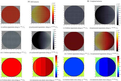
The contour plots of the UE and polynomial eigenstrains (UE + IPE) for stiff and compliant inclusions are shown in Figure 8(A-i, A-ii, A-iii, A-iv) and Figure 8 (B-i, B-ii, B-iii, B-iv), respectively. The induced elastic stress plots in the dominant direction σ^e_yy for the stiff and compliant inclusions are shown in Figure 8(A-v, A-vi) and Figure 8 (B-v, B-vi), respectively.

Figure 8. Eigenstrains and induced elastic stress field. (A) Stiff inclusion, (B) Compliant inclusion. Both (A) and (B) (i) Uniform eigenstrains along xx  ^{UE} ε*_xx. (ii) Polynomial eigenstrains along xx ^{UE+IPE} ε*_xx. (iii) Uniform eigenstrains along yy ^{UE} ε*_yy. (iv) Polynomial eigenstrains along yy ^{UE+IPE} ε*_yy. (v) Uniform elastic stress along yy ^{UE}σ^e_yy. (vi) Interaction case elastic stress along yy ^{UE+IPE}σ^e_yy.

5.2.3. Plots for perturbation in density of distributed dislocations (PDD)

The perturbations in the dislocation density are obtained using the solution of IPE coefficients and Equations (28a) and (28b). Using polynomial representation of cubic degree with four terms to represent the unknown field of eigenstrains, the bounded functions determined from Equation (7a) are shown in Figure 9(a,b) for stiff and compliant inclusion interaction with the crack. The results show that the perturbation in dislocation density (PDD) has the opposite sense to the distributed dislocation density from the applied loads (KD) for a stiff inclusion. Hence, the crack is shielded by a stiff inclusion. For a compliant inclusion, the PDD has the same sense as KD, and the stress intensity factor is amplified.

Figure 9. Computation of density of distributed dislocation. (a) Stiff inclusion interaction. (b) Compliant inclusion interaction.

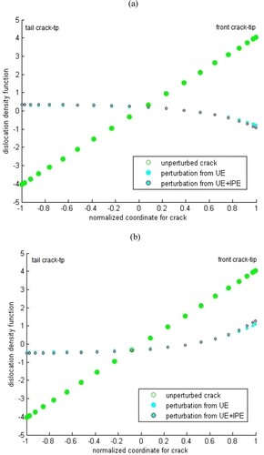
For the stiff and compliant inclusions, the contribution from uniform eigenstrains on perturbations in distributed dislocations (UDD) has the same sense as PDD. The strength of UDD and PDD is significantly greater for the front crack tip than the tail crack tip. Furthermore, the plots in Figure 9(a,b) show that IPDD contribution (difference between PDD and UDD) on the crack face is maximum at the front crack-tip, for stiff and compliant inclusions.

5.3. Results for perturbed stress intensity factor

The numerical results [18,55] to quantify the interaction due to inclusion on mode I crack are expressed in the normalized perturbed stress intensity factor defined as follows. (36a) $\begin{array}{rl}{K}_{I(n)}^{SOL}(\pm 1)& =1+\frac{\mathrm{\Delta }{K_I}^{SOL}(\pm 1)}{\sqrt{\pi a}{{\sigma }_{22}}^{(app)}}\end{array}$(36a) (36b) $\begin{array}{rl}\mathrm{\Delta }{K_I}^{SOL}(\pm 1)& =\sqrt{\pi a}\left[\frac{2{\mu }_1}{({\kappa }_1+1)}\right][{\phi }^{SOL}(\pm 1)]\end{array}$(36b) (36c) $\begin{array}{rl}\phi (\pm 1{)}^{SOL}& =[{}^{\{UE\}}{\phi }^{SOL}(\pm 1)+{}^{\{IPE\}}{\phi }^{SOL}(\pm 1)]\end{array}$(36c) where the denominator represents the (unperturbed) classical stress intensity factor for mode I crack, K_I(n) = 13.5358 Nmm ^−3/2, and in the numerator, ΔK_I (+1)^SOL and ΔK_I (−1)^SOL are perturbations in stress intensity factors due to the interaction, for the front crack tip and tail crack tip, respectively. Furthermore, ϕ^SOL(+1) and ϕ^SOL(−1) in equation (36c) are perturbations in dislocation density computed at the crack-tips and based on distributed dislocations on the crack face (UDD + IPDD) with expression given in reference [41,42]. The results (Table 2) for stiff and compliant inclusions for various geometric configurations have good accuracy compared to benchmark results of Rooke and Cartwright [55].

Table 2. Perturbed SIF for ρ = 2a and various h/ρ.

	Inclusion modulus ratio µ2/µ1 Stiff
Clear separation h/ρ	inclusion 3.0	Compliant inclusion 0.333
.20	0.771	1.321
	0.770 [45]	1.325 [45]
0.5	0.893	1.149
	0.890 [45]	1.155 [45]
1	0.952	1.067
	0.950 [45]	1.070 [45]

6. Discussion and concluding remarks

The eigenstrains inside an inclusion are always non-uniform due to mutual elastic interaction with the crack. Furthermore, the IPE are quantitative measures of the interaction field since the unknown coefficients of IPE form the only unknowns.

To ensure numerical convergence, the redundant eigenstrain terms in polynomial representation for IPE need to be avoided [34,35]. For the interaction configuration involving single crack and single inclusion, the higher-order eigenstrain terms are expected to be predominantly odd-powered [46]. But, for interaction configuration such as  two equal cracks and one inclusion placed symmetrically or in periodic setting,the higher-order eigenstrain terms are expected to be quadratic or predominantly even-powered [45]. Thus, the accuracy of the numerical solution is limited by ill-posedness and also depends on the representation for the IPE.

However, when the representation for the eigenstrains has an exact polynomial, two added benefits can be redeemed in the numerical solution: first, the interaction stress field solution becomes exact in Equation (26); second, the boundary condition at the inclusion boundary is also satisfied in Equation (31). Therefore, the reconstruction solution suggests a careful selection of a polynomial representation of IPE based on the prior information of the elastic field for a particular problem [36,39,46]. For modulus ratios involving extreme values of soft or hard inclusions, the error scales with the value of uniform eigenstrains, for each geometric configuration. Thus, for a void, the maximum error is about 3 times the values in Table 2 or about 2% for a clear separation of 0.2. Since shear eigenstrains are omitted (Section 5.1.3), for smaller clear separation, the error is expected to be higher. The addition of higher-order terms encounters non-convergence. However, the percentage contribution from polynomial eigenstrains to perturbation in SIF is modest. It is about 15% for clear separation of 0.2, implying that uniform eigenstrain solution shall introduce about 15% error in SIF computation (Table 3). The sense of influence (shielding or amplification) on perturbations in distributed dislocations on the crack face and SIF because of the contributions due to the elastic interaction from polynomial eigenstrains and uniform eigenstrain for a stiff or compliant inclusion are shown in Figure 9.

Table 3. Induced polynomial eigenstrain contribution to ΔK_I (+1) with (ρ/a = 2.0, µ₂/µ₁ = 3.0).

	Contributions to perturbation in SIF for front crack-tip
Normalized clear separation h/ρ	1 − KI(n)(+1)^SOL	uniform eigenstrain term	induced polynomial eigenstrain term	contribution of induced polynomial eigenstrain
0.2	0.229	0.195	0.034	14.9%
0.5	0.107	0.103	0.004	3.7%
1.0	0.048	0.048	< 0.001	0.0%

In sum, the present formulation derives the interaction stress field solution using superposition, based on two semi-analytical techniques, namely, EIM to model the inclusion and DDT to model the crack. The numerical solution is obtained based on the coefficients of the unknown field of IPE inside the inclusion as the only unknowns. Through a careful selection of IPE representation that avoids redundant terms, only four terms are used to obtain a reasonable accuracy for stiff and compliant inclusions for moderate geometric configurations. The formulation identifies the unknown IPE as a complete measure of the interaction field strength to capture amplification or shielding quantitatively.

Acknowledgements

Comments from Dr David Hill are gratefully acknowledged to modify the paper. The author thanks Mechanical Engineering department and the Computer Centre, IIT Kanpur for the support in carrying the simulations. 

Disclosure statement

No potential conflict of interest was reported by the author(s).

Additional information

Funding

This work did not receive any specific grant or financial sponsorship. 

Appendices

Appendix 1. Column vector for unknown coefficients of IPE

In vector notation, uniform eigenstrains can be expressed by the column of three elements as follows. (A1) $\{{}^{\{UE\}}{\epsilon }^{\ast }{\}}_{1X3}={\left\{\begin{array}{ccc}{}^{\{UE\}}{\epsilon }_{xx}^{\ast }& {}^{\{UE\}}{\epsilon }_{yy}^{\ast }& {}^{\{UE\}}{\epsilon }_{xy}^{\ast }\end{array}\right\}}^T$(A1) Re-expressing Equations (5a)–(5c), polynomial eigenstrains in Equation (11) can be represented by a column vector, with elements denoting the unknown component terms as follows. (A2) $\begin{array}{rl}\{{}^{\{IPE\}}\epsilon {}^{\ast }{\}}_{3\mathrm{\Pi }X1}& ={\left\{\begin{array}{ccccc}\{{}^{\{1\}}{\epsilon }^{\ast }\}& \dots & \{{}^{\{p\}}{\epsilon }^{\ast }\}& \dots & \{{}^{\{\mathrm{\Pi }\}}{\epsilon }^{\ast }\}\end{array}\right\}}^T\end{array}$(A2) (A3) $\begin{array}{rl}\{{}^{\{p\}}{\epsilon }^{\ast }{\}}_{1X3}& =A_p(x,y)\left\{\begin{array}{ccc}{\alpha }_p{}^{\{UE\}}{\epsilon }_{xx}^{\ast }& {\beta }_p{}^{\{UE\}}{\epsilon }_{yy}^{\ast }& {\gamma }_e{}^{\{UE\}}{\epsilon }_{xy}^{\ast }\end{array}\right\}\end{array}$(A3) where index p = 1Π, denotes the sequence-index for polynomial eigenstrains’ representation shown in Equations (5a)–(5c). In Equation (A1.3), the unknown coefficients corresponding to index p are α_p β_p and γ_p . The terms A_p depend on the coordinates (x,y) for a point inside the inclusion. In inverse-EIM formulation, the polynomial coefficients are selected as the unknowns to be determined numerically. The unknowns in Equation (A1.3) can be expressed by a column vector of 3Π elements as shown below. (A4) $\begin{array}{rl}\{{}^{\{IPE\}}\mathrm{\Theta }{\}}_{3\mathrm{\Pi }x1}& ={\left\{\begin{array}{ccccc}\{{\mathrm{\Theta }}_1\}& \dots & \{{\mathrm{\Theta }}_p\}& \dots & \{{\mathrm{\Theta }}_{\mathrm{\Pi }}\}\end{array}\right\}}^T\end{array}$(A4) (A5) $\begin{array}{rl}\{{\mathrm{\Theta }}_p{\}}_{3x1}& =\left\{\begin{array}{ccc}{\alpha }_p& {\beta }_p& {\gamma }_p\end{array}\right\}\end{array}$(A5) Equations (A4) and (A5) are useful since, in EIM formulation, the induced elastic field of each eigenstrain term can be algebraically added to compute the cumulative contribution.

2

Numerical computation using Gauss–Chebyshev quadrature

For computing the perturbations in the density of distributed dislocations (PDD) from Equations (21)–(23), crack-face tractions in Eequation (20) are used. The crack-face tractions are computed by summation of stress field contributions on the crack-face from point loads, F₁⁽ⁱ⁾ and F₂ ⁽ⁱ⁾ at inclusion boundary given by Equations (12b) and (13), corresponding to each eigenstrain term (UE + IPE).

Based on the terminology introduced in Section 4.2.2, the perturbations in the density of distributed dislocations because of uniform eigenstrains (UDD) and polynomial eigenstrains (IPDD) in Equation (21) can be expressed as follows: (A6) $\begin{array}{rl}{}^{\{UE\}}\phi ({\zeta }^{(\tau )})& =G_1{}^{\{UE\}}{\epsilon }^{\ast }\end{array}$(A6) (A7) $\begin{array}{rl}{}^{\{IPE\}}\phi ({\zeta }^{(\tau )})& =G_2{}^{\{IPE\}}{\epsilon }^{\ast }\end{array}$(A7) where (A8) $\begin{array}{rl}{G}_1& ={\left\{\begin{array}{ccc}{}^{\{UE\}}{\mathrm{\Phi }}_1^{(\tau )}& {}^{\{UE\}}{\mathrm{\Phi }}_2^{(\tau )}& {}^{\{UE\}}{\mathrm{\Phi }}_3^{(\tau )}\end{array}\right\}}_{1x3}\end{array}$(A8) (A9) $\begin{array}{rl}{G}_2& ={\left\{\begin{array}{ccccc}\{{}^{\{IPE\}}{\mathrm{\Phi }}_1^{(\tau )}\}& \dots & \{{}^{\{IPE\}}{\mathrm{\Phi }}_p^{(\tau )}\}& \dots & \{{}^{\{IPE\}}{\mathrm{\Phi }}_{\mathrm{\Pi }}^{(\tau )}\}\end{array}\right\}}_{1x3\mathrm{\Pi }}\end{array}$(A9) (A10) $\begin{array}{rl}{}^{\{IPE\}}{\mathrm{\Phi }}_p^{(\tau )}& ={\left\{\begin{array}{ccc}{}_p^{\{\alpha \}}\mathrm{\Phi }({\zeta }^{(\tau )})& {}_p^{\{\beta \}}\mathrm{\Phi }({\zeta }^{(\tau )})& {}_p^{\{\gamma \}}\mathrm{\Phi }({\zeta }^{(\tau )})\end{array}\right\}}_{1x3}\end{array}$(A10) where ^{UE}Φ^(τ) and ^{ΙPE}Φ^(τ) are computed from the numerical solution through Gauss–Chebyshev Quadrature formula at discrete points on crack face with coordinates ζ^(τ). Equations (A6) and (A8) obtain the distributed dislocations because of the uniform eigenstrains (UDD, synonymous with UE). Similarly, Equations (A7) and (A9) obtain distributed dislocations because of the polynomial eigenstrains (IPDD, synonymous with IPE), by adding the contributions from each term with index p = 1 … Π.

References

- Bush MB. The interaction between a crack and a particle cluster. Int J Frac. 1997;88:215–232.
- Huang J, Rapoff AJ, Haftka RT. Attracting cracks for arrestment in bonelike composites. Mater Design. 2006;27:461–469.
- Mantic V. Interfacial crack onset at a circular cylindrical inclusion under a remote transverse tension, application of a coupled stress and energy criterion. Int J Solids Struct. 2009;46:1287–1304.
- Barsoum RS. On the use of isoparametric finite elements in linear fracture mechanics. Int J Num Methods Eng. 1976;10:25–37.
- Atluri SN. Computational Methods in Mechanics of Fracture, Vol 2. Amsterdam: North-Holland; 1986.
- Daux C, Moes N, Dolbow J, et al. Arbitrary branched and intersecting cracks with the extended finite element method. Int J Num Methods Eng. 2000;48:1741–1760.
- Cruse TA. BIE fracture mechanics analysis: 25 years of developments. Comp Mech. 1996;18:1–11.
- Aliabadi MH, Rooke DP. Numerical fracture mechanics (Solid mechanics and its applications; Vol 8). Dordrecht: Kluwer Academic Pub; 1991.
- Silveira NPP, Guimaraes S, Telles JCF. A numerical green’s function BEM formulation for crack growth initiation. Eng Anal Bound Elem. 2005;29:978–985.
- Mews H, Kuhn G. An effective numerical stress intensity factor calculation with no crack discretization. Int J Frac. 1988;38:61–76.
- Ma J, Chen W, Zhang C, et al. Meshless simulation of anti-plane crack problems by the method of fundamental solutions using the crack Green’s function. Comput Math Appl. 2020;79:1543–1560.
- Lin J, Feng W, Reutskiy S, et al. A new semi-analytical method for solving a class of time fractional partial differential equations with variable coefficients. Appl Math Lett. 2021;112(106712.
- Kitey R, Phan A-V, Tippur HV, et al. Modeling of crack growth through particulate clusters in brittle matrix by symmetric-Galerkin boundary element method. Int J Frac. 2006;141:11–25.
- Wang J, Crouch SL, Mogilevskaya SG. A fast and accurate algorithm for a Galerkin boundary integral method. Comput Mech. 2005;37:96–109.
- Han X, Wang T. Elastic fields of interacting elliptic inhomogeneities. Int J Solids Struct. 1999;36:4523–4541.
- Tamate O. The effect of a circular inclusion on the stresses around a line crack in a sheet under tension. Int J Frac Mech. 1968;4:257–266.
- Atkinson C. The interaction between and crack and an inclusion. Int J Eng Sci. 1972;10:127–136.
- Erdogan F, Gupta GD, Ratwani M. Interaction between a circular inclusion and an arbitrarily oriented crack. ASME J Appl Mech. 1974; Dec: 1007-1013.
- Patton EM, Santare MH. Crack path prediction near an elliptic inclusion. Eng Frac Mech. 1993;44:195–205.
- Arai M. Application of distributed dislocation method to curved crack moving near a press-fitted inclusion in a two-dimensional infinite plate. Eng Frac Mech. 2019;218:106609.
- Wang R. A new method for calculating the stress intensity factors of a crack with a circular inclusion. Acta Mech. 1995;108:77–85.
- Li Z, Chen Q. Crack-inclusion interaction for mode I crack analyzed by Eshelby equivalent inclusion method. Int J Frac. 2002;118:29–40.
- Shodja HM, Rad IZ, Soheilifard R. Interacting cracks and ellipsoidal inhomogeneities by the equivalent inclusion method. J Mech Phy Solids. 2003;51:945–960.
- Moschovidis ZA, Mura T. Two-ellipsoidal inhomogeneities by the equivalent inclusion method. ASME J Appl Mech. 1975;42:847–852.
- Eshelby JD. Ealstic Inclusions and Inhomogeneities. In: Sneddon IN, Hill R, editors. Progresses in Solid Mechanics Vol II. Amsterdam: North-Holland Pub; 1961. p. 89–140.
- Eshelby JD. The determination of the elastic field of an ellipsoidal inclusion and related problems. R Soc Lond A. 1957;214:376–396.
- Mura T. Micromechanics of defects in solids. 2nd ed. Dordrecht: Martinus Nijhoff Pub; 1987.
- Lubarda VA, Markenscoff X. On absence of esehlby property for non-ellipsoidal inclusions. Int J Solids Struct. 1998;35:3405–3411.
- Asaro RJ, Barnett DM. The non-uniform transformation strain problem for an anisotropic ellipsoidal inclusion. J Mech Phys Solids. 1975;23:77–83.
- Jun T-S, Korsunsky AM. Evaluation of residual stresses and strains using eigenstrain reconstruction method. Int J Solids Struct. 2010;47:1678–1686.
- Chen YZ. Solution for Eshelby’s elliptic inclusion with polynomials distribution of the eigenstrains in plane elasticity. Appl Math Model. 2014;38:4872–4884.
- Lee Y-G, Zuo W-N, Pan E. Eshelby’s problem of polygonal inclusions with polynomial eigenstrains in an anisotropic megneto-electro-elastic full plane. Proc R Soc A. 2015;471:1–20.
- Rahman M. The isotropic ellipsoidal inclusion with polynomial distribution of eigenstrains. ASME J Appl Mech. 2002;69:593–601.
- Kabaanikhin SI. Definitions and examples of inverse and ill-posed problems. J Inv Ill-Posed Probl. 2008;16:317–357.
- Bonnet M, Constantinescu A. Inverse problems in elasticity. Inverse Prob. 2005;21:R1–R50.
- Cao YP, Hu N, Lu J, et al. An inverse approach for constructing the residual stress field induced by wielding. J Strain Anal Eng Des. 2002;37:345–359.
- Hill MR. Determination of residual stress based on the estimation of eigenstrain [PhD thesis]. Stanford: Stanford University; 1996.
- Korsunsky AM, Regino GM, Nowell D. Variational eigenstrain analysis of residual stresses in a welded plate. Int J Solids and Str. 2007;44:4574–4591.
- Agrawal A. Eigenstrain reconstruction from contaminated data using inverse-EIM. 4th Int Conf Struct Integrity, Madeira; Aug-Sept 2021.
- Bilby BA, Eshelby JD. Dislocations and the theory of fracture. In; Liebowitz S, editor. Fracture, microscopic and macroscopic fundamentals. Vol. 1, Academic Press; 1969. p. 99–182.
- Hills DA, Kelly PA, Dai DN, Korsunsky AM. Solution of crack problem: the distributed dislocation technique. In Gladwell GML, editor, Solid mechanics and its applications. Dordrecht: Springer; 1996.
- Krenk S. On the Use of the interpolation polynomials for solutions of singular integral equations. Quant Appl Math. 1975;32:479–484.
- Mausavi MS, Lazar M. Distributed dislocation technique for cracks based on non-singular dislocations in nonlocal elasticity of Helmholtz type. Eng Fract Mech. 2015;136:79–95.
- Jin X, Lyu D, Zhang X, et al. Explicit analytical solutions for a complete set of Eshelby tensors of an ellipsoidal inclusion. ASME J Appl Mech. 2016;83:1–12.
- Song G, Wang L, Deng L, et al. Mechanical characterization and inclusion based boundary element modeling of lightweight concrete containing foam particles. Mech Mater. 2015;91:208–225.
- Agrawal A, Venkitanarayanan P. Polynomial selection for induced eigenstrain inside a stiff inclusion interacting strongly with a mode I crack. MCM Conference; Sept 2017; Petersburg, Russia.
- Gladwell GML. Contact problems in the classical theory of elasticity. Sijthoff Noordhoff. 1980.
- Jen E, Srivastava RP. Solving singular integral equations using Gaussian quadrature and over-determined systems. Comput Math Appl. 1983;9:625–632.
- Mushkhelishvili NI. Some basic problems of the mathematical theory of elasticity. Springer-Science; 1953.
- Chen YZ. Integral equations methods for multiple crack problems and related topics. ASME J Appl Mech. 2007;60:172–194.
- Newman JC. An improved method of collocation for stress analysis of cracked plates with various shaped boundaries. NASATN D-6376. 1971; NASA.
- Wang YH. Stress intensity factor for a crack in a tube by boundary collocation method. Int J Press Vessels Pip. 1989;38:167–176.
- MATLAB. Mathworks Inc, Natick, Massachusetts, 2014.
- Lin J, Zhang Y, Reutskiy S, et al. A novel meshless space-time backward substitution method and its application to nonhomogeneous advection-diffusion problems. Appl Math Comput. 2021;398:125964.
- Rooke DP, Cartwright DJ. 1975. Compendium of stress intensity factors. London: Her Majesty’s Stationary Office.