A finite-difference and Haar wavelets hybrid collocation technique for non-linear inverse Cauchy problems

ABSTRACT

In this research work, a finite-difference and Haar wavelet hybrid collocation scheme is introduced for the ill-posed non-linear inverse Cauchy problem with a source depending on space variable along with an unknown solution and unknown right side boundary. The first-order finite-difference approach is adopted to approximate the $\frac{\mathrm{\partial }u}{\mathrm{\partial }t}$ part and two different Haar series are managed to approximate $\frac{{\mathrm{\partial }}^{2}u}{\mathrm{\partial }{x}^2}$ part and source term respectively. A simple linearization procedure is used to convert the non-linear problem into a linear form. In contradiction to various numerical schemes, the current introduced method generates a well-conditioned system of algebraic equations, therefore it is not required to apply a regularization approach. The results of the proposed method are stable and converge to the exact solution. Some numerical tests are also performed to confirm the accuracy, well-conditioning of the algebraic equations and easy applicability of the scheme on linear and non-linear cases.

KEYWORDS:

• Inverse Cauchy problems
• Haar wavelets
• collocation method
• non-linear problems
• source term

MATHS:

• 35-02
• 35-04
• 35-11

1. Introduction

Inverse problems in which the unknown heat source or densities, the coefficients present in the governing parabolic partial differential equation (PDE), some unknown part of the boundary conditions involved in a mathematical model under investigation are not easy to determine accurately and therefore a lot of researchers trying to find these types of unknown parameters. The identification of these types of parameters in PDEs with the help of an extra information called overspecified condition performs an influential role in physics, engineering sciences and applied mathematics. It will be very easy to solve the inverse problem if the initial information and boundary information are known exactly along with the overspecified condition. However, in practical cases, these information are not accurately available, because the design is then maintained in an antagonistic situation so that the temperature cannot be measured at the initial time, or the estimation of boundary information in the inaccessible section of the surface is not allowed.

In this article, we discussed the non-linear inverse Cauchy problem (NLICP) to recover the unknown source term depending on space variable ($H(x)$) for one-dimensional parabolic PDE [1]: (1) $\begin{array}{rl}& \frac{\mathrm{\partial }u(x,t)}{\mathrm{\partial }t}=\frac{{\mathrm{\partial }}^{2}u(x,t)}{\mathrm{\partial }{x}^2}-\kappa {\left(\frac{\mathrm{\partial }u(x,t)}{\mathrm{\partial }x}\right)}^2+H(x),x\in (0,\ell ),t\in (0,T),\end{array}$(1) (2) $\begin{array}{rl}& u(x,0)=u_o(x),(\mathrm{measured}\mathrm{initial}\mathrm{information}),\end{array}$(2) (3) $\begin{array}{rl}& u(0,t)=f(t),(\mathrm{measured}\mathrm{temperature}\mathrm{on}\mathrm{left}\mathrm{side}),\end{array}$(3) (4) $\begin{array}{rl}& \frac{\mathrm{\partial }u(0,t)}{\mathrm{\partial }x}=g(t),(\mathrm{measured}\mathrm{flux}\mathrm{on}\mathrm{left}\mathrm{side}),\end{array}$(4) where $u(x,t)$ is the state variable, H is the heat source depending on the x direction only, κ is some constant ($\kappa =0$ for linear case otherwise non-linear), ℓ is the length of the interval and T is the final time. The change with time and the diffusion of state variable are denoted by $\frac{\mathrm{\partial }u(x,t)}{\mathrm{\partial }t}$ and $\frac{{\mathrm{\partial }}^{2}u(x,t)}{\mathrm{\partial }{x}^2}$ respectively where as $(\frac{\mathrm{\partial }u(x,t)}{\mathrm{\partial }x}{)}^2$ is the non-linear convection term. Equation (1(1) $\begin{array}{rl}& \frac{\mathrm{\partial }u(x,t)}{\mathrm{\partial }t}=\frac{{\mathrm{\partial }}^{2}u(x,t)}{\mathrm{\partial }{x}^2}-\kappa {\left(\frac{\mathrm{\partial }u(x,t)}{\mathrm{\partial }x}\right)}^2+H(x),x\in (0,\ell ),t\in (0,T),\end{array}$(1) )–(4(4) $\begin{array}{rl}& \frac{\mathrm{\partial }u(0,t)}{\mathrm{\partial }x}=g(t),(\mathrm{measured}\mathrm{flux}\mathrm{on}\mathrm{left}\mathrm{side}),\end{array}$(4) ) is a Cauchy problem because given information are defined in left-end boundary. This parabolic PDE possesses seven main difficulties for numerical technique: Cauchy boundary conditions, non-linearity, ill-posedness, ill-conditioning, unknown solution, unknown heat source and unknown right-end boundary. A complete solution of (1(1) $\begin{array}{rl}& \frac{\mathrm{\partial }u(x,t)}{\mathrm{\partial }t}=\frac{{\mathrm{\partial }}^{2}u(x,t)}{\mathrm{\partial }{x}^2}-\kappa {\left(\frac{\mathrm{\partial }u(x,t)}{\mathrm{\partial }x}\right)}^2+H(x),x\in (0,\ell ),t\in (0,T),\end{array}$(1) )–(4(4) $\begin{array}{rl}& \frac{\mathrm{\partial }u(0,t)}{\mathrm{\partial }x}=g(t),(\mathrm{measured}\mathrm{flux}\mathrm{on}\mathrm{left}\mathrm{side}),\end{array}$(4) ) will be $u(x,t)$, $H(x)$ and $u(\ell ,t)$. Due to ill-posedness this problem is very sensitive to the small error in the input data and is also very much challenging to solve numerically due to the non-linearity. In general, recovery of the these unknowns in non-linear inverse problem is not possible without overspecified conditions. These required additional information are usually collected from empirical observations. In experiment the device/sensor is already maintained in an antagonistic situation due to which the experimental observations (overspecified conditions) contain some amount of error (noise) and numerical approaches usually produce unstable and inaccurate solutions. To obtain these unknowns accurately, we assume the overspecified conditions (heat flux) at an initial time: (5) $\frac{\mathrm{\partial }u(x,0)}{\mathrm{\partial }x}=u_o^{\prime }(x),(\mathrm{flux}\mathrm{at}\mathrm{initial}\mathrm{time}(\mathrm{overspecified}\mathrm{condition})).$(5) Calculating stable numerical results is difficult but by adopting some kind of regularization procedure similar to Tikhonov regularization, discrepancy principal or the L-curve criterion [2] can reduce the instabilities. Computational and mathematical complications are reported in [3–17] due to the ill-posedness and ill-conditioning of the inverse problems and the results are unstable. Few of the particular latest numerical programs published in different journals related to inverse heat PDEs are boundary element (BEM) [2], RBF methods [18,19], iterative regularization technique [20], Lie-group method (LGM) [21] and method of fundamental solution (MFS) [22,23]. Some recent contribution to the inverse problems are reported in [24–26].

The diffusion and dispersion of pollution at any instant in a watershed can be mathematically represented by the linear parabolic equation. The following parabolic equation is a spacial case to the model equation (1(1) $\begin{array}{rl}& \frac{\mathrm{\partial }u(x,t)}{\mathrm{\partial }t}=\frac{{\mathrm{\partial }}^{2}u(x,t)}{\mathrm{\partial }{x}^2}-\kappa {\left(\frac{\mathrm{\partial }u(x,t)}{\mathrm{\partial }x}\right)}^2+H(x),x\in (0,\ell ),t\in (0,T),\end{array}$(1) ) and is known as the groundwater pollution equation [27] $\frac{\mathrm{\partial }u(x,t)}{\mathrm{\partial }t}=s_1\frac{{\mathrm{\partial }}^{2}u(x,t)}{\mathrm{\partial }{x}^2}-s_2\frac{\mathrm{\partial }u(x,t)}{\mathrm{\partial }x}-s_{3}u(x,t)+P(x,t),$with the given information $\{\begin{array}{l}u(x,0)=0,(\text{initial condition}),\\ u(0,t)=u(\pi ,t)=0,(\text{boundray conditions}),\\ u(x,T)=g(x),(\text{overspecified condition given at final time T}),\end{array}$where the unknown function $u(x,t)$ is the concentration of pollution, $s_1$ is the diffusion coefficient, $s_2$ is average velocity of water in a watershed, $s_3$ is the self-purifying function of the watershed, $g(x)$ is known function and $P(x,t)$ is the pollution source. This equation has been analysed for different types of space and time dependent source terms in [27,28].

For linear inverse heat equation there are many articles with different source term, like Cannon and Duchateau have found $H(u)$ in [29]. Siraj-ul-islam and Muhammad Ahsan have identified time dependent heat source $H(t)$ [30] and $F(x)$ [31] accurately by Haar wavelet collocation method (HWCM). The same author Siraj-ul-islam have also identified time dependent heat source H(t) accurately by meshless collocation method [18]. Lesnic has calculated heat source depending on space variable ($F(x)$) in [2] and the thermal conductivity $a(t)>0$ in [32]. Chein-Shan Liu has used homogenized function method to find time-space separable source ($F(x,t)=H(t)+G(x)$) [33]. Hasanov calculated $H(t)$ and $F(x)$ independently from the source ($F(x)H(t)$) in [28]. However, there are only one research paper [1] to solve this NLICP (1(1) $\begin{array}{rl}& \frac{\mathrm{\partial }u(x,t)}{\mathrm{\partial }t}=\frac{{\mathrm{\partial }}^{2}u(x,t)}{\mathrm{\partial }{x}^2}-\kappa {\left(\frac{\mathrm{\partial }u(x,t)}{\mathrm{\partial }x}\right)}^2+H(x),x\in (0,\ell ),t\in (0,T),\end{array}$(1) ) under conditions (2(2) $\begin{array}{rl}& u(x,0)=u_o(x),(\mathrm{measured}\mathrm{initial}\mathrm{information}),\end{array}$(2) ), (3(3) $\begin{array}{rl}& u(0,t)=f(t),(\mathrm{measured}\mathrm{temperature}\mathrm{on}\mathrm{left}\mathrm{side}),\end{array}$(3) ), (4(4) $\begin{array}{rl}& \frac{\mathrm{\partial }u(0,t)}{\mathrm{\partial }x}=g(t),(\mathrm{measured}\mathrm{flux}\mathrm{on}\mathrm{left}\mathrm{side}),\end{array}$(4) ) and (5(5) $\frac{\mathrm{\partial }u(x,0)}{\mathrm{\partial }x}=u_o^{\prime }(x),(\mathrm{flux}\mathrm{at}\mathrm{initial}\mathrm{time}(\mathrm{overspecified}\mathrm{condition})).$(5) ). Hence the current research work for NLICP is a challenging and non-classical one.

Different sorts of inverse Cauchy problems have been examined for the particular interest. Inverse Cauchy problem of Laplace and biharmonic equations are handled by the local method of fundamental solution recently in [34]. Inverse problem with Cauchy data has been solved by boundary function method in [35]. Heat conduction problem in non-linear functionally graded materials has been solved by meshless method [36].

Utilizing Haar wavelets in numerical approximation have become an advanced trend recently. The detailed calculations related to the Haar wavelets are studied in weak and strong formulations, that include Daubechies wavelet-based approach [37], wavelet meshless strategies [38,39], wavelet collocation schemes [40–43] and wavelet Galerkin approach [44]. The implementation of the wavelets-related numerical method for various types of PDEs can be observed in [45]. The complete detail of some of the Haar wavelets numerical estimation techniques for distinctive sorts of integral as well as differential equations have addressed in [46–63]. The numerical strategy based on Haar wavelets has also been boosted for non-linear single, coupled and frictional PDEs in [64–70].

1.1. Inverse problems and Haar wavelet-based method

Haar wavelets have been used to solve linear type of inverse problems. One-dimensional inverse problem with unknown boundary condition has been analysed in [71], where the term $\frac{{\mathrm{\partial }}^{3}u(x,t)}{\mathrm{\partial }t\mathrm{\partial }{x}^2}$ has been approximated by Haar wavelets just to find the numerical solution in the unit interval $[0,1]$. Two-dimensional parabolic and hyperbolic inverse problems are solved in [72], where $\frac{{\mathrm{\partial }}^{5}u(x,y,t)}{\mathrm{\partial }t\mathrm{\partial }{x}^2\mathrm{\partial }{y}^2}$ and $\frac{{\mathrm{\partial }}^{6}u(x,y,t)}{{\mathrm{\partial }}^{2}t\mathrm{\partial }{x}^2\mathrm{\partial }{y}^2}$ are approximated by Haar wavelets for parabolic and hyperbolic problems respectively. Inverse problems with unknown source terms are solved with HWCM, where the non-homogeneous inverse problems have been converted into homogeneous form by eliminating the time dependent as well as space dependent source term with suitable transformation in one and two-dimensions [30,31]. In [30] the HWCM capture continuous, discontinuous and oscillatory source terms accurately. The control parameter in the inverse problem is determined by HWCM recently with efficient and accurate results [73].

1.2. The main objective of this study

In this study, our main objective is to solve the ill-posed NILCP with unknown source term via finite-difference formula combined with Haar wavelets series for the first time. The presence of non-linear part in (1(1) $\begin{array}{rl}& \frac{\mathrm{\partial }u(x,t)}{\mathrm{\partial }t}=\frac{{\mathrm{\partial }}^{2}u(x,t)}{\mathrm{\partial }{x}^2}-\kappa {\left(\frac{\mathrm{\partial }u(x,t)}{\mathrm{\partial }x}\right)}^2+H(x),x\in (0,\ell ),t\in (0,T),\end{array}$(1) ) is strenuous to tackle numerically but can be handled by the linearization process. This ill-posed linearized equation is converted into well-conditioned system of algebraic equation without regularization procedure with the help of Haar wavelets and then solved for $u(x,t)$, $H(x)$ and $u(\ell ,t)$ for different intensity of noise levels. This technique is easy, reliable and efficient to solve NLICPs. Due to the well condition behaviour of the algebraic equations, we do not need to initiate any type of regularization procedure to the current HWCM.

In this proposed technique the first-order finite-difference estimation is followed for time derivative and two distinctive Haar wavelets combinations are employed to approximate the source term and space derivative. Due to the piecewise continuity of the Haar wavelets, the highest-order derivative in (1(1) $\begin{array}{rl}& \frac{\mathrm{\partial }u(x,t)}{\mathrm{\partial }t}=\frac{{\mathrm{\partial }}^{2}u(x,t)}{\mathrm{\partial }{x}^2}-\kappa {\left(\frac{\mathrm{\partial }u(x,t)}{\mathrm{\partial }x}\right)}^2+H(x),x\in (0,\ell ),t\in (0,T),\end{array}$(1) ) is estimated by the Haar series. The Haar series is then integrated to get the required expressions for the first-order derivative and of the solution. A system of linear equations is formed as a result of these approximations.

The remaining part of this paper can further be classified into different sections. In Section 2, Haar functions are defined. In Section 3, the Haar wavelet-based numerical technique is presented. Result and discussion are performed in Section 4.

2. Haar wavelets

A Haar wavelet family for $x\in [0,\ell )$ is defined as (6) $h_i(x)=\{\begin{array}{ll}1& \mathrm{if}x\in [{\phi }_1(i),{\phi }_2(i)),\\ -1& \mathrm{if}x\in [{\phi }_2(i),{\phi }_3(i)),\\ 0& \mathrm{otherwise},\end{array}$(6) where ${\phi }_1(i)=\frac{\ell k}{m},{\phi }_2(i)=\frac{\ell (k+0.5)}{m},\mathrm{and}{\phi }_3(i)=\frac{\ell (k+1)}{m}.$Let $\begin{array}{rl}{p}_{i,1}(x)& ={\int }_0^x{h}_i(x^{\prime })\mathrm{d}{x}^{\prime },\\ p_{i,2}(x)& ={\int }_0^x{p}_{i,1}(x^{\prime })\mathrm{d}{x}^{\prime },\end{array}$and $C_i={\int }_0^1{p}_{i,1}(x^{\prime })\mathrm{d}{x}^{\prime }.$Using (6(6) $h_i(x)=\{\begin{array}{ll}1& \mathrm{if}x\in [{\phi }_1(i),{\phi }_2(i)),\\ -1& \mathrm{if}x\in [{\phi }_2(i),{\phi }_3(i)),\\ 0& \mathrm{otherwise},\end{array}$(6) ), we get $\begin{array}{rl}{p}_{i,1}(x)& =\{\begin{array}{ll}x-{\phi }_1(i)& \mathrm{if}x\in [{\phi }_1(i),{\phi }_2(i)),\\ x-{\phi }_1(i)-2(x-{\phi }_2(i))& \mathrm{if}x\in [{\phi }_2(i),{\phi }_3(i)),\\ x-{\phi }_1(i)-2(x-{\phi }_2(i))+(x-{\phi }_3(i))& \mathrm{if}x\in [{\phi }_3(i),\ell ),\\ 0& \mathrm{otherwise},\end{array}\\ p_{i,2}(x)& =\{\begin{array}{ll}\frac{1}{2}(x-{\phi }_1(i){)}^2& \mathrm{if}x\in [{\phi }_1(i),{\phi }_2(i)),\\ \frac{1}{2}((x-{\phi }_1(i){)}^2-2(x-{\phi }_2(i){)}^2)& \mathrm{if}x\in [{\phi }_2(i),{\phi }_3(i)),\\ \frac{1}{2}((x-{\phi }_1(i){)}^2-2(x-{\phi }_2(i){)}^2+(x-{\phi }_3(i){)}^2)& \mathrm{if}x\in [{\phi }_3(i),\ell ),\\ 0& \mathrm{otherwise},\end{array}\end{array}$and $C_i=\frac{\ell }{4m^2}.$In the above function $m=2^j,j=0,1,\dots ,J$ shows different level of the wavelet and $k=0,1,\dots ,m-1$ shows the translating parameter. The highest level of resolution is represented by J. The index i in Equation (6(6) $h_i(x)=\{\begin{array}{ll}1& \mathrm{if}x\in [{\phi }_1(i),{\phi }_2(i)),\\ -1& \mathrm{if}x\in [{\phi }_2(i),{\phi }_3(i)),\\ 0& \mathrm{otherwise},\end{array}$(6) ) can be obtained with the help of equation i = m + k + 1. For smallest values of m = 1 we can obtain k = 0 and the index i = 2. The largest value of index i is $M=2^J$. Here we can also present the Haar wavelets scaling function as $h_1(x)=\{\begin{array}{ll}1& \mathrm{if}x\in [0,\ell ),\\ 0& \mathrm{otherwise}.\end{array}$

3. Haar wavelets scheme for NLICP

To construct a numerical scheme based on Haar wavelet for (1(1) $\begin{array}{rl}& \frac{\mathrm{\partial }u(x,t)}{\mathrm{\partial }t}=\frac{{\mathrm{\partial }}^{2}u(x,t)}{\mathrm{\partial }{x}^2}-\kappa {\left(\frac{\mathrm{\partial }u(x,t)}{\mathrm{\partial }x}\right)}^2+H(x),x\in (0,\ell ),t\in (0,T),\end{array}$(1) ), we estimated the highest-order derivative and the heat source in (1(1) $\begin{array}{rl}& \frac{\mathrm{\partial }u(x,t)}{\mathrm{\partial }t}=\frac{{\mathrm{\partial }}^{2}u(x,t)}{\mathrm{\partial }{x}^2}-\kappa {\left(\frac{\mathrm{\partial }u(x,t)}{\mathrm{\partial }x}\right)}^2+H(x),x\in (0,\ell ),t\in (0,T),\end{array}$(1) ) by two different finite Haar wavelet series as; (7) $\begin{array}{rl}& \frac{{\mathrm{\partial }}^{2}u(x,t)}{\mathrm{\partial }{x}^2}\approx \sum _{i=1}^{2M}{\lambda }_i{h}_i(x),\end{array}$(7) (8) $\begin{array}{rl}& H(x)\approx \sum _{i=1}^{2M}{\rho }_i{h}_i(x),\end{array}$(8) here ${\lambda }_i$ and ${\rho }_i$ are unknown Haar coefficients. Integrating (7(7) $\begin{array}{rl}& \frac{{\mathrm{\partial }}^{2}u(x,t)}{\mathrm{\partial }{x}^2}\approx \sum _{i=1}^{2M}{\lambda }_i{h}_i(x),\end{array}$(7) ) with respect to x from 0 to x, we acquire (9) $\frac{\mathrm{\partial }u(x,t)}{\mathrm{\partial }x}\approx \frac{\mathrm{\partial }u(0,t)}{\mathrm{\partial }x}+\sum _{i=1}^{2M}{\lambda }_i{p}_{i,1}(x).$(9) Putting (4(4) $\begin{array}{rl}& \frac{\mathrm{\partial }u(0,t)}{\mathrm{\partial }x}=g(t),(\mathrm{measured}\mathrm{flux}\mathrm{on}\mathrm{left}\mathrm{side}),\end{array}$(4) ) in (9(9) $\frac{\mathrm{\partial }u(x,t)}{\mathrm{\partial }x}\approx \frac{\mathrm{\partial }u(0,t)}{\mathrm{\partial }x}+\sum _{i=1}^{2M}{\lambda }_i{p}_{i,1}(x).$(9) ) and then integrating from 0 to x, we acquire (10) $u(x,t)\approx u(0,t)+xg(t)+\sum _{i=1}^{2M}{\lambda }_i{p}_{i,2}(x).$(10) Introducing the well-known implicit scheme for Equation (1(1) $\begin{array}{rl}& \frac{\mathrm{\partial }u(x,t)}{\mathrm{\partial }t}=\frac{{\mathrm{\partial }}^{2}u(x,t)}{\mathrm{\partial }{x}^2}-\kappa {\left(\frac{\mathrm{\partial }u(x,t)}{\mathrm{\partial }x}\right)}^2+H(x),x\in (0,\ell ),t\in (0,T),\end{array}$(1) ), we get ${\left(\frac{\mathrm{\partial }u(x,t)}{\mathrm{\partial }t}\right)}^{j+1}={\left(\frac{{\mathrm{\partial }}^{2}u(x,t)}{\mathrm{\partial }{x}^2}\right)}^{j+1}-\kappa {\left({\left(\frac{\mathrm{\partial }u(x,t)}{\mathrm{\partial }x}\right)}^2\right)}^{j+1}+(H(x){)}^{j+1}.$Using first-order accurate finite-difference estimation for time derivative $(\frac{\mathrm{\partial }u(x,t)}{\mathrm{\partial }t}{)}^{j+1}=\frac{(u(x,t){)}^{j+1}-(u(x,t){)}^j}{\mathrm{\Delta }t}+\mathcal{O}(\mathrm{\Delta }t)$, we get (11) $\begin{array}{rl}& (u(x,t){)}^{j+1}-\mathrm{\Delta }t{\left(\frac{{\mathrm{\partial }}^{2}u(x,t)}{\mathrm{\partial }{x}^2}\right)}^{j+1}+\kappa \mathrm{\Delta }t{\left({\left(\frac{\mathrm{\partial }u(x,t)}{\mathrm{\partial }x}\right)}^2\right)}^{j+1}-\mathrm{\Delta }t(H(x){)}^{j+1}\\ & =(u(x,t){)}^j+\mathcal{O}(\mathrm{\Delta }t).\end{array}$(11) Linearizing the non-linear term in the following manner, which can be obtained using the Taylor expansion [74,75] (12) $\begin{array}{rl}{\left({\left(\frac{\mathrm{\partial }u(x,t)}{\mathrm{\partial }x}\right)}^2\right)}^{j+1}& ={\left(\frac{\mathrm{\partial }u(x,t)}{\mathrm{\partial }x}\right)}^{j+1}{\left(\frac{\mathrm{\partial }u(x,t)}{\mathrm{\partial }x}\right)}^{j+1}\\ & ={\left(\frac{\mathrm{\partial }u(x,t)}{\mathrm{\partial }x}\right)}^j{\left(\frac{\mathrm{\partial }u(x,t)}{\mathrm{\partial }x}\right)}^{j+1}+{\left(\frac{\mathrm{\partial }u(x,t)}{\mathrm{\partial }x}\right)}^{j+1}{\left(\frac{\mathrm{\partial }u(x,t)}{\mathrm{\partial }x}\right)}^j\\ & -{\left(\frac{\mathrm{\partial }u(x,t)}{\mathrm{\partial }x}\right)}^j{\left(\frac{\mathrm{\partial }u(x,t)}{\mathrm{\partial }x}\right)}^j\\ & =2{\left(\frac{\mathrm{\partial }u(x,t)}{\mathrm{\partial }x}\right)}^j{\left(\frac{\mathrm{\partial }u(x,t)}{\mathrm{\partial }x}\right)}^{j+1}-{\left({\left(\frac{\mathrm{\partial }u(x,t)}{\mathrm{\partial }x}\right)}^2\right)}^j.\end{array}$(12) Putting (12(12) $\begin{array}{rl}{\left({\left(\frac{\mathrm{\partial }u(x,t)}{\mathrm{\partial }x}\right)}^2\right)}^{j+1}& ={\left(\frac{\mathrm{\partial }u(x,t)}{\mathrm{\partial }x}\right)}^{j+1}{\left(\frac{\mathrm{\partial }u(x,t)}{\mathrm{\partial }x}\right)}^{j+1}\\ & ={\left(\frac{\mathrm{\partial }u(x,t)}{\mathrm{\partial }x}\right)}^j{\left(\frac{\mathrm{\partial }u(x,t)}{\mathrm{\partial }x}\right)}^{j+1}+{\left(\frac{\mathrm{\partial }u(x,t)}{\mathrm{\partial }x}\right)}^{j+1}{\left(\frac{\mathrm{\partial }u(x,t)}{\mathrm{\partial }x}\right)}^j\\ & -{\left(\frac{\mathrm{\partial }u(x,t)}{\mathrm{\partial }x}\right)}^j{\left(\frac{\mathrm{\partial }u(x,t)}{\mathrm{\partial }x}\right)}^j\\ & =2{\left(\frac{\mathrm{\partial }u(x,t)}{\mathrm{\partial }x}\right)}^j{\left(\frac{\mathrm{\partial }u(x,t)}{\mathrm{\partial }x}\right)}^{j+1}-{\left({\left(\frac{\mathrm{\partial }u(x,t)}{\mathrm{\partial }x}\right)}^2\right)}^j.\end{array}$(12) ) in (11(11) $\begin{array}{rl}& (u(x,t){)}^{j+1}-\mathrm{\Delta }t{\left(\frac{{\mathrm{\partial }}^{2}u(x,t)}{\mathrm{\partial }{x}^2}\right)}^{j+1}+\kappa \mathrm{\Delta }t{\left({\left(\frac{\mathrm{\partial }u(x,t)}{\mathrm{\partial }x}\right)}^2\right)}^{j+1}-\mathrm{\Delta }t(H(x){)}^{j+1}\\ & =(u(x,t){)}^j+\mathcal{O}(\mathrm{\Delta }t).\end{array}$(11) ) we get (13) $\begin{array}{rl}& (u(x,t){)}^{j+1}-\mathrm{\Delta }t{\left(\frac{{\mathrm{\partial }}^{2}u(x,t)}{\mathrm{\partial }{x}^2}\right)}^{j+1}+2\kappa \mathrm{\Delta }t{\left(\frac{\mathrm{\partial }u(x,t)}{\mathrm{\partial }x}\right)}^j{\left(\frac{\mathrm{\partial }u(x,t)}{\mathrm{\partial }x}\right)}^{j+1}-\mathrm{\Delta }t(H(x){)}^{j+1}\\ & =(u(x,t){)}^j+\kappa \mathrm{\Delta }t{\left({\left(\frac{\mathrm{\partial }u(x,t)}{\mathrm{\partial }x}\right)}^2\right)}^j+\mathcal{O}(\mathrm{\Delta }t).\end{array}$(13) Dropping the local truncation error $\mathcal{O}(\mathrm{\Delta }t)$ for time approximation and putting (7(7) $\begin{array}{rl}& \frac{{\mathrm{\partial }}^{2}u(x,t)}{\mathrm{\partial }{x}^2}\approx \sum _{i=1}^{2M}{\lambda }_i{h}_i(x),\end{array}$(7) ), (9(9) $\frac{\mathrm{\partial }u(x,t)}{\mathrm{\partial }x}\approx \frac{\mathrm{\partial }u(0,t)}{\mathrm{\partial }x}+\sum _{i=1}^{2M}{\lambda }_i{p}_{i,1}(x).$(9) ), (10(10) $u(x,t)\approx u(0,t)+xg(t)+\sum _{i=1}^{2M}{\lambda }_i{p}_{i,2}(x).$(10) ) and (8(8) $\begin{array}{rl}& H(x)\approx \sum _{i=1}^{2M}{\rho }_i{h}_i(x),\end{array}$(8) ) in (13(13) $\begin{array}{rl}& (u(x,t){)}^{j+1}-\mathrm{\Delta }t{\left(\frac{{\mathrm{\partial }}^{2}u(x,t)}{\mathrm{\partial }{x}^2}\right)}^{j+1}+2\kappa \mathrm{\Delta }t{\left(\frac{\mathrm{\partial }u(x,t)}{\mathrm{\partial }x}\right)}^j{\left(\frac{\mathrm{\partial }u(x,t)}{\mathrm{\partial }x}\right)}^{j+1}-\mathrm{\Delta }t(H(x){)}^{j+1}\\ & =(u(x,t){)}^j+\kappa \mathrm{\Delta }t{\left({\left(\frac{\mathrm{\partial }u(x,t)}{\mathrm{\partial }x}\right)}^2\right)}^j+\mathcal{O}(\mathrm{\Delta }t).\end{array}$(13) ) and further simplification, we get (14) $\begin{array}{rl}& \sum _{i=1}^{2M}{\lambda }_i(p_{i,2}(x)-\mathrm{\Delta }t{h}_i(x)+2\kappa \mathrm{\Delta }t{\left(\frac{\mathrm{\partial }u(x,t)}{\mathrm{\partial }x}\right)}^j{p}_{i,1}(x))-\mathrm{\Delta }t\sum _{i=1}^{2M}{\rho }_i{h}_i(x)\\ & =(u(x,t){)}^j+\kappa {\left({\left(\frac{\mathrm{\partial }u(x,t)}{\mathrm{\partial }x}\right)}^2\right)}^j-(f(t)+xg(t))-2\kappa \mathrm{\Delta }tg(t){\left(\frac{\mathrm{\partial }u(x,t)}{\mathrm{\partial }x}\right)}^j.\end{array}$(14) The matrix representation of (14(14) $\begin{array}{rl}& \sum _{i=1}^{2M}{\lambda }_i(p_{i,2}(x)-\mathrm{\Delta }t{h}_i(x)+2\kappa \mathrm{\Delta }t{\left(\frac{\mathrm{\partial }u(x,t)}{\mathrm{\partial }x}\right)}^j{p}_{i,1}(x))-\mathrm{\Delta }t\sum _{i=1}^{2M}{\rho }_i{h}_i(x)\\ & =(u(x,t){)}^j+\kappa {\left({\left(\frac{\mathrm{\partial }u(x,t)}{\mathrm{\partial }x}\right)}^2\right)}^j-(f(t)+xg(t))-2\kappa \mathrm{\Delta }tg(t){\left(\frac{\mathrm{\partial }u(x,t)}{\mathrm{\partial }x}\right)}^j.\end{array}$(14) ) is (15) $\begin{array}{rl}& ({\mathbf{P}}_2-\mathrm{\Delta }t\mathbf{H}+2\kappa \mathrm{\Delta }t{\mathbf{U}\mathbf{x}}_o{\mathbf{P}}_1)\mathit{\lambda }-(\mathrm{\Delta }t\mathbf{H})\mathit{\rho }\\ & ={\mathbf{u}}_o+\kappa ({\mathbf{U}\mathbf{x}}_o{)}^2-(f(t)+\mathbf{x}g(t))-2\kappa \mathrm{\Delta }tg(t){\mathbf{U}\mathbf{x}}_o,\end{array}$(15) where $\begin{array}{rl}& \mathbf{x}=[x_1,x_2,\dots ,x_{2M}{]}^T,\mathit{\lambda }=[{\lambda }_1,{\lambda }_2,\dots ,{\lambda }_{2M}{]}^T,\mathit{\rho }=[{\rho }_1,{\rho }_2,\dots ,{\rho }_{2M}{]}^T,\\ & {\mathbf{u}}_o=[u(x_1,t),u(x_2,t),\dots ,u(x_{2M},t){]}^T,{\mathbf{U}\mathbf{x}}_o=[u_x(x_1,t),u_x(x_2,t),\dots ,u_x(x_{2M},t)],\\ & \mathbf{H}=\left[\begin{array}{cccc}{h}_1(x_1)& h_2(x_1)& \dots & h_{2M}(x_1)\\ h_1(x_2)& h_2(x_2)& \dots & h_{2M}(x_2)\\ \dots & \dots & \dots & \dots \\ h_1(x_{2M})& h_2(x_{2M})& \dots & h_{2M}(x_{2M})\end{array}\right],\\ & {\mathbf{P}}_1=\left[\begin{array}{cccc}{P}_{1,1}(x_1)& P_{2,1}(x_1)& \dots & P_{2M,1}(x_1)\\ P_{1,1}(x_2)& P_{2,1}(x_2)& \dots & P_{2M,1}(x_2)\\ \dots & \dots & \dots & \dots \\ P_{1,1}(x_{2M})& P_{2,1}(x_{2M})& \dots & P_{2M,1}(x_{2M})\end{array}\right],\end{array}$and ${\mathbf{P}}_2=\left[\begin{array}{cccc}{P}_{1,2}(x_1)& P_{2,2}(x_1)& \dots & P_{2M,2}(x_1)\\ P_{1,2}(x_2)& P_{2,2}(x_2)& \dots & P_{2M,2}(x_2)\\ \dots & \dots & \dots & \dots \\ P_{1,2}(x_{2M})& P_{2,2}(x_{2M})& \dots & P_{2M,2}(x_{2M})\end{array}\right].$Now using the overspecified condition (5(5) $\frac{\mathrm{\partial }u(x,0)}{\mathrm{\partial }x}=u_o^{\prime }(x),(\mathrm{flux}\mathrm{at}\mathrm{initial}\mathrm{time}(\mathrm{overspecified}\mathrm{condition})).$(5) ) in (9(9) $\frac{\mathrm{\partial }u(x,t)}{\mathrm{\partial }x}\approx \frac{\mathrm{\partial }u(0,t)}{\mathrm{\partial }x}+\sum _{i=1}^{2M}{\lambda }_i{p}_{i,1}(x).$(9) ) we get (16) $\sum _{i=1}^{2M}{\lambda }_i{p}_{i,1}(x)=u_o^{\prime }(x)-g(0).$(16) The matrix representation of (16(16) $\sum _{i=1}^{2M}{\lambda }_i{p}_{i,1}(x)=u_o^{\prime }(x)-g(0).$(16) ) is (17) ${\mathbf{P}}_1\mathit{\lambda }=u_o^{\prime }(\mathbf{x})-g(0).$(17) The two systems (15(15) $\begin{array}{rl}& ({\mathbf{P}}_2-\mathrm{\Delta }t\mathbf{H}+2\kappa \mathrm{\Delta }t{\mathbf{U}\mathbf{x}}_o{\mathbf{P}}_1)\mathit{\lambda }-(\mathrm{\Delta }t\mathbf{H})\mathit{\rho }\\ & ={\mathbf{u}}_o+\kappa ({\mathbf{U}\mathbf{x}}_o{)}^2-(f(t)+\mathbf{x}g(t))-2\kappa \mathrm{\Delta }tg(t){\mathbf{U}\mathbf{x}}_o,\end{array}$(15) ) and (17(17) ${\mathbf{P}}_1\mathit{\lambda }=u_o^{\prime }(\mathbf{x})-g(0).$(17) ) can be composed in the matrix form (18) $\mathbf{A}\mathbf{X}\mathbf{=}\mathbf{B},$(18) where $\mathbf{A}=\left(\begin{array}{cc}{\mathbf{P}}_2-\mathrm{\Delta }t\mathbf{H}+2\kappa \mathrm{\Delta }t{\mathbf{U}\mathbf{x}}_o{\mathbf{P}}_1& -\mathrm{\Delta }t\mathbf{H}\\ {\mathbf{P}}_1& 0\end{array}\right),\mathbf{X}=\left(\begin{array}{c}\mathit{\lambda }\\ \mathit{\rho }\end{array}\right)$and $\mathbf{B}=\left(\begin{array}{c}{\mathbf{u}}_o+\kappa {\mathbf{U}\mathbf{x}}_o^2-(f(t)+\mathbf{x}g(t))-2\kappa \mathrm{\Delta }tg(t){\mathbf{U}\mathbf{x}}_o\\ u_o^{\prime }(\mathbf{x})-g(0)\end{array}\right).$Equation (18(18) $\mathbf{A}\mathbf{X}\mathbf{=}\mathbf{B},$(18) ) can be solved by appropriate linear solver like Gaussian elimination method and plucking back the values of X in (10(10) $u(x,t)\approx u(0,t)+xg(t)+\sum _{i=1}^{2M}{\lambda }_i{p}_{i,2}(x).$(10) ) and (8(8) $\begin{array}{rl}& H(x)\approx \sum _{i=1}^{2M}{\rho }_i{h}_i(x),\end{array}$(8) ) one can find the numerical solution and numerical heat source. The right boundary $u(\ell ,t)$ can be easily calculated from (10(10) $u(x,t)\approx u(0,t)+xg(t)+\sum _{i=1}^{2M}{\lambda }_i{p}_{i,2}(x).$(10) ) by putting $x=\ell$.

4. Convergence of HWCM

Theorem 4.1

Assume that $\mathrm{\partial }u/\mathrm{\partial }t$, ${\mathrm{\partial }}^{k}u/\mathrm{\partial }{x}^k$, k = 1, 2, 3, exist and are bounded in the given interval. For any $M=2^J$, $J=0,1,2,\dots$, if $u_M(x)$ is the Haar wavelet solution and $u(x,t)$ is the exact solution then $\Vert u(x,t)-u_M(x){\Vert }_{\mathrm{\infty }}\le \mathcal{O}{\left(\frac{1}{2^{J+1}}\right)}^2+\mathcal{O}(\mathrm{\Delta }t)\mathrm{as}J\to \mathrm{\infty }\mathrm{and}\mathrm{\Delta }t\to 0.$

Proof.

For space discretization see [76,77] and we have used forward difference approximation for time derivative which is first-order accurate in time discretization i.e. $\mathcal{O}(\mathrm{\Delta }t)$ (look at Equation (13(13) $\begin{array}{rl}& (u(x,t){)}^{j+1}-\mathrm{\Delta }t{\left(\frac{{\mathrm{\partial }}^{2}u(x,t)}{\mathrm{\partial }{x}^2}\right)}^{j+1}+2\kappa \mathrm{\Delta }t{\left(\frac{\mathrm{\partial }u(x,t)}{\mathrm{\partial }x}\right)}^j{\left(\frac{\mathrm{\partial }u(x,t)}{\mathrm{\partial }x}\right)}^{j+1}-\mathrm{\Delta }t(H(x){)}^{j+1}\\ & =(u(x,t){)}^j+\kappa \mathrm{\Delta }t{\left({\left(\frac{\mathrm{\partial }u(x,t)}{\mathrm{\partial }x}\right)}^2\right)}^j+\mathcal{O}(\mathrm{\Delta }t).\end{array}$(13) )). Hence $\Vert u(x,t)-u_M(x){\Vert }_{\mathrm{\infty }}\to 0$, as J$\to \mathrm{\infty }\mathrm{and}\mathrm{\Delta }t\to 0$.

5. Computational results

To investigate the performance of the HWCM in response to the non-linear inverse Cauchy problem, we introduce noisy data on initial, all boundaries and overspecified conditions as (19) $\begin{array}{rl}& \overline{u}(x,0)=u_o(x)+\sigma r,\\ & \overline{u}(0,t)=f(t)+\sigma r,\\ & \frac{\mathrm{\partial }\overline{u}(0,t)}{\mathrm{\partial }x}=g(t)+\sigma r,\\ & \frac{\mathrm{\partial }\overline{u}(x,0)}{\mathrm{\partial }x}=u_o^{\prime }(x)+\sigma r,\end{array}$(19) where σ represents the amount of noise levels and 0<r<1 is the arbitrary real number calculated by the command rand in MATLAB. We adopted M = 16, $\mathrm{\Delta }t=0.01$ and T = 1 for all the computations otherwise mentioned their. For the precision and efficiency of the HWCM, we have applied the maximum absolute error ($L_{\mathrm{\infty }}$) and the experimental rate of convergence ($R_c$) [63], which are defined as $\begin{array}{rl}& L_{\mathrm{\infty }}(S_M)=\mathrm{Max}(|S_M-S_M^{\ast }|),\\ & R_c(S_M)=\frac{\log [L_{\mathrm{\infty }}(S_{\frac{M}{2}})/L_{\mathrm{\infty }}(S_M)]}{\log (2)},\end{array}$where $S^{\ast }$ and S describe numerical and exact values sequentially, M is number of collocation points and S is either u or H.

The condition number of a matrix measures the sensitivity of the matrix, like how much error be there in the output results for a small error in the input data. A matrix with a high condition number means that the determinant of the matrix is close to zero and is difficult to find its inverse accurately and hence the numerical results are unstable. The condition number of a $\mathbf{A}$ can be mathematically defined as $\kappa (\mathbf{A})=\frac{{\delta }_{max}(\mathbf{A})}{{\delta }_{min}(\mathbf{A})},$where ${\delta }_{max}(\mathbf{A})$ and ${\delta }_{min}(\mathbf{A})$ are maximal and minimal singular values of $\mathbf{A}$ respectively and $\kappa (\mathbf{A})$ can be easily calculated by using the built-in command cond(A) in MATLAB${}^{\circledR }$.

5.1. Numerical results for linear inverse Cauchy problems

In this subsection we have consider two test example for verification of the proposed HWCM for different types of heat source.

Example 5.1

trigonometric heat source

Considering the linear case of Equation (1(1) $\begin{array}{rl}& \frac{\mathrm{\partial }u(x,t)}{\mathrm{\partial }t}=\frac{{\mathrm{\partial }}^{2}u(x,t)}{\mathrm{\partial }{x}^2}-\kappa {\left(\frac{\mathrm{\partial }u(x,t)}{\mathrm{\partial }x}\right)}^2+H(x),x\in (0,\ell ),t\in (0,T),\end{array}$(1) ) as $\kappa =0$ on interval length $\ell =1$. The initial and boundary conditions are $u_o(x)=x^2+\sin (2\pi x)$, $f(t)=0$, $g(t)=2t+2\pi$ respectively. The overspecified condition is $u_o^{\prime }(x)=2\pi \cos (2\pi x)$+2x. The exact solution is $u(x,t)=x(x+2t)+\sin (2\pi x)$ and exact heat source is $H(x)=2(x-1+2{\pi }^2\sin (2\pi x))$.

In Table 1, the maximum errors $L_{\mathrm{\infty }}$ for u and H are given along with conditional number of matrix A. As the number of collocation points M increases the $L_{\mathrm{\infty }}$ errors decrease. The performance of the HWCM is more reliable due to the well-conditioned behaviour of the Haar coefficient matrix A, therefore it is not required to use any regularization technique. In Figure 1, the comparison of numerical and exact solution (u and H) are presented along with the absolute errors at large noise level $\sigma =10\mathrm{\%}$ which are very close to each other.

Figure 1. Comparison of HWCM and exact solution for Test Problem 5.1, at M = 128, $\sigma =10\mathrm{\%}$.

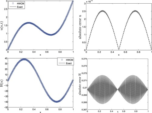
Table 1. The $L_{\mathrm{\infty }}$ errors and condition number for $\mathrm{\Delta }t=0.01$ and T = 1 at various M, Test Problem 5.1.

M	$L_{\mathrm{\infty }}(u)$	$L_{\mathrm{\infty }}(H)$	$L_{\mathrm{\infty }}(u)$	$L_{\mathrm{\infty }}(H)$	$\kappa (\mathbf{A})$
	$\sigma =0.01$		$\sigma =0.001$
2	2.885e−01	2.844e+01	2.885e−01	2.844e+01	1.224e+02
4	4.332e−02	1.027e+01	4.333e−02	1.028e+01	3.603e+02
8	8.438e−03	4.441e+00	8.439e−03	4.444e+00	1.821e+03
16	1.848e−03	2.066e+00	1.849e−03	2.071e+00	1.010e+04
32	4.311e−04	9.888e−01	4.315e−04	1.000e+00	5.693e+04
64	1.039e−04	4.669e−01	1.040e−04	4.899e−01	3.217e+05
128	2.546e−05	1.930e−01	2.555e−05	2.391e−01	1.819e+06

The performance of the proposed HWCM has also been shown in Table 2 for different $\mathrm{\Delta }t$ with fixed T = 5. Table 3 shows the relationships of increasing the spatial discretization unit ($\ell /2M$) on the findings. As the length of the interval ℓ is divided into $2M$ collocation points and by incensing the ℓ and fixing M, the space discretization unit rises and affects the numerical computation.

Table 2. The $L_{\mathrm{\infty }}$ errors at $\sigma =0.01$ and T = 5, Test Problem 5.1.

M	$L_{\mathrm{\infty }}(u)$	$L_{\mathrm{\infty }}(H)$	CPU time	$L_{\mathrm{\infty }}(u)$	$L_{\mathrm{\infty }}(H)$	CPU time
	$\mathrm{\Delta }t=0.1$			$\mathrm{\Delta }t=0.001$
2	2.886e−01	2.849e+01	0.108	2.880e−01	2.837e+01	4.124
4	4.342e−02	1.112e+01	0.304	4.308e−02	1.015e+01	7.914
8	8.590e−03	4.638e+00	1.423	8.289e−03	4.137e+00	14.234
16	1.941e−03	1.560e+00	5.075	1.798e−03	1.652e+00	31.722
32	4.390e−04	9.936e−01	10.507	4.301e−04	9.559e−01	59.918
64	1.249e−04	6.030e−01	21.268	9.127e−05	3.838e−01	82.538

Table 3. The $L_{\mathrm{\infty }}$ errors at M = 32, $\mathrm{\Delta }t=0.05$, $\sigma =5\mathrm{\%}$ and T = 2, Test Problem 5.1.

	$\ell =1$	$\ell =2$	$\ell =3$	$\ell =4$	$\ell =5$
$L_{\mathrm{\infty }}(u)$	4.295e−04	1.845e−03	4.478e−03	8.431e−03	1.434e−02
$L_{\mathrm{\infty }}(H)$	9.3766e−01	2.040e+00	3.199e+00	4.428e+00	5.767e+00
$\ell /2M=\ell /64$	0.0156	0.0313	0.0469	0.0625	0.0781

Example 5.2

Smooth heat source

Considering Equation (1(1) $\begin{array}{rl}& \frac{\mathrm{\partial }u(x,t)}{\mathrm{\partial }t}=\frac{{\mathrm{\partial }}^{2}u(x,t)}{\mathrm{\partial }{x}^2}-\kappa {\left(\frac{\mathrm{\partial }u(x,t)}{\mathrm{\partial }x}\right)}^2+H(x),x\in (0,\ell ),t\in (0,T),\end{array}$(1) ) with the parameters $\kappa =0$ and $\ell =1.5$. The exact solution and linear heat source are $u(x,t)=t+(x-0.5{)}^3,H(x)=4-6x.$The initial, boundary and overspecified conditions can be calculated from the exact solution. The recovered u, H and $u(\ell ,t)$ for $\sigma =1\mathrm{\%}$ are compared with exact one in Figure 2, which are essentially coincident with each other having the maximum errors $5.827\times {10}^{-4}$, $7.031\times {10}^{-2}$ and $2.500\times {10}^{-4}$ respectively. To observe the performance of the HWCM, we introduce different amounts of noise level σ to initial, boundary and overspecified conditions that are the perturbation of the available information, effect the numerical results slightly. In Table 4 the maximum errors $L_{\mathrm{\infty }}$ for u, H and $u(\ell ,t)$ along with rate of convergence are given for different values of σ, which shows that the results of HWCM are correct and the accuracy increases by incensing the number of collocation points M. The numerical results converges to the exact solution and hence the HWCM handle linear inverse Cauchy problem.

Figure 2. Comparison of HWCM results and exact solution for Test Problem 5.2.

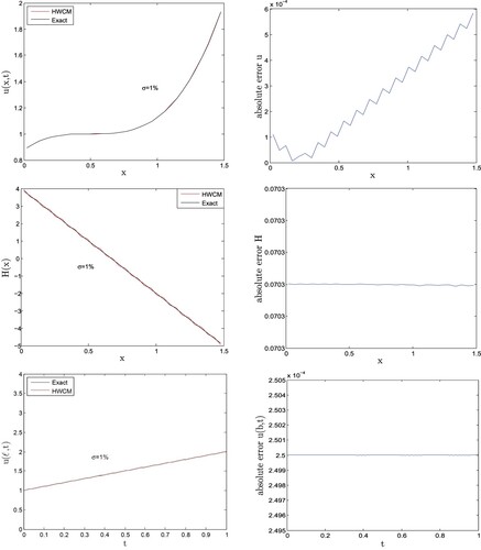
Table 4. The $L_{\mathrm{\infty }}$ errors and rate of convergence for $\mathrm{\Delta }t=0.01$ and T = 1 at various M, Test Problem 5.2.

M	$L_{\mathrm{\infty }}(u)$	$L_{\mathrm{\infty }}(H)$	$L_{\mathrm{\infty }}(u(\ell ,t))$	$L_{\mathrm{\infty }}(u)$	$L_{\mathrm{\infty }}(H)$	$R_c(u_M)$	$R_c(H_M)$
	$\sigma =0.01$			$\sigma =0.1$		$\sigma =0.01$
2	5.579e−2	5.625e−1	2.500e−4	5.371e−2	5.625e−1	–	–
4	1.335e−2	2.812e−1	2.500e−4	1.118e−2	2.812e−1	2.0632	1.0003
8	3.102e−3	1.406e−1	2.500e−4	1.098e−3	1.406e−1	2.1056	1.0000
16	5.827e−4	7.031e−2	2.500e−4	1.663e−3	7.031e−2	2.4124	0.9998
32	1.019e−4	3.515e−2	2.500e−4	2.281e−3	3.515e−2	2.5156	1.0002

5.2. Numerical results for non-linear inverse Cauchy problems

On successful implementation on linear problems, we are also presenting the non-linear inverse heat problems results for different cases.

Example 5.3

Algebraic heat source

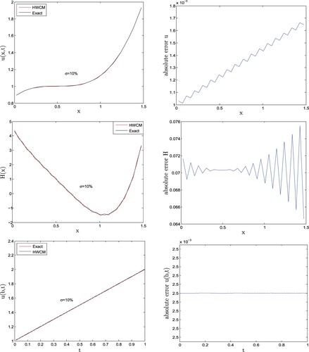
Let us consider a non-linear inverse Cauchy problem with $\kappa =1$. The exact representations for $u(x,t)$and $H(x)$ are $u(x,t)={(x-\frac{1}{2})}^3+t,H(x)=9{(x-\frac{1}{2})}^4+1-6(x-\frac{1}{2}).$The given data can be obtained from the exact solution. In this case, we take $\ell =1.5$ to compare the HWCM results with Lie-group algebraic equations method (LGAM)[1]. In Figure 3, the comparison shows that the results of HWCM are more accurate than LGAM. The maximum error of H(x) for $\sigma =0.001$ and $\sigma =0.05$ reported in [1] are 0.04 and 1.27 where as for the same noise level the maximum errors of HWCM are 0.0704 and 0.0729 which means that HWCM handle this NLICP accurately on large noise data. For this problem we have also consider $\sigma =10\mathrm{\%}$ and the considerable accurate result of this large amount of polluted data are given in Figure 4.

Figure 3. Comparison of LGAM [1] and HWCM for Test Problem 5.3.

Figure 4. Comparison of HWCM results and exact solution for Test Problem 5.3.

To cheeked the influence of noise σ on $\mathbf{A}$ defined in Equation (18(18) $\mathbf{A}\mathbf{X}\mathbf{=}\mathbf{B},$(18) ), we perturbed $\mathbf{A}$ by $\sigma \mathbf{A}$ and $\mathbf{A}+\sigma \mathbf{I}$, where $\mathbf{I}$ is matrix of ones with same size of $\mathbf{A}$. Table 5 shows the condition number of $\mathbf{A}$ as well as its perturbed forms, where the condition number of $\mathbf{A}$ effected slightly by the various noise quantities and this is the beauty of the proposed HWCM.

Table 5. The condition number of perturbed $\mathbf{A}$ at different noise amount σ, M = 32, T = 0.1 and $\mathrm{\Delta }t=0.01$, Test Problem 5.3.

	$\sigma =0.01$	$\sigma =0.1$	$\sigma =1$	$\sigma =5$	$\sigma =10$
$\kappa (\mathbf{A})$	1.6355e+05	1.6362e+05	1.6365e+05	1.6765e+05	1.6924e+05
$\kappa (\sigma \mathbf{A})$	1.6355e+05	1.6362e+05	1.6365e+05	1.6765e+05	1.6924e+05
$\kappa (\mathbf{A}+\sigma \mathbf{I})$	1.5345e+05	1.5833e+05	3.0417e+05	01.3285e+06	2.6333e+06

Example 5.4

Trigonometric heat source

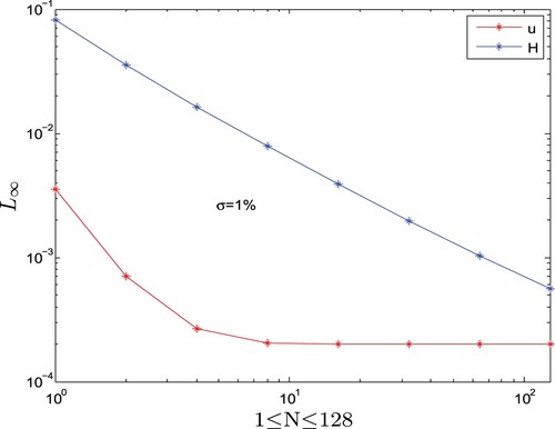
Let us consider a non-linear inverse Cauchy problem with $\kappa =1$ and $\ell =1$. The exact representations for $u(x,t)$and $H(x)$ are $u(x,t)=t+\cos (x-\frac{1}{2}),H(x)=\sin {(x-\frac{1}{2})}^2+\cos (x-\frac{1}{2})+1.$The given data can be obtained from the exact solution. The maximum errors for u and H under a noise with $\sigma =1\mathrm{\%}$ are given in Figure 5, which proves that the HWCM is more reliable and handle this non-linear inverse Cauchy problem as well.

Figure 5. The $L_{\mathrm{\infty }}$ for Test Problem 5.4.

Example 5.5

Quadratic heat source

Again considering the non-linear inverse Cauchy problem with $\kappa =1$ and $\ell =1$. The exact description for $u(x,t)$and $H(x)$ are $u(x,t)=t-(x^2-0.5),H(x)=4x^2+3.$For this non-linear problem we have considered $\sigma =20\mathrm{\%}$ and the considerable accurate result of this large amount of polluted data are given in Table 6, where the error goes to reduce by increasing the number of collocation points M. Comparison of HWCM results with the exact solution under noise intensity $\sigma =10\mathrm{\%}$ are shown in Figure 6, which are almost coincident with each others.

Figure 6. Comparison of HWCM results with the exact solution under $\sigma =10\mathrm{\%}$ for Test Problem 5.5.

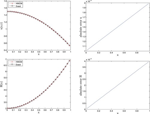
Table 6. The $L_{\mathrm{\infty }}$ errors for $\mathrm{\Delta }t=0.01$ and T = 1 at various M, Test Problem 5.5.

M	$L_{\mathrm{\infty }}(u)$	$L_{\mathrm{\infty }}(H)$	$L_{\mathrm{\infty }}(u)$	$L_{\mathrm{\infty }}(H)$
	$\sigma =0.01$		$\sigma =0.2$
2	1.984e−4	3.937e−4	3.968e−3	7.871e−3
4	1.968e−4	3.874e−4	3.937e−3	7.746e−3
8	1.937e−4	3.749e−4	3.874e−3	7.495e−3
16	1.874e−4	3.499e−4	3.749e−3	6.995e−3

Example 5.6

Exponential heat source

Finally considering the non-linear inverse Cauchy problem with exponential heat source along with $\kappa =1$ and $\ell =1$. The solution and heat source in this case are $u(x,t)=t+e^{(2x+1)},H(x)=4e^{(4x+2)}-4e^{(2x+1)}+1.$For this non-linear problem we have considered noise intensity $\sigma =10\mathrm{\%}$ and the considerable accurate result of this large amount of polluted data are given in Table 7. Comparison of HWCM results with the exact solution under noise intensity $\sigma =20\mathrm{\%}$ are shown in Figure 7, which are almost coincident with each others. The numerical results converges to the exact solution for different level of noise intensity and the error decreases by increasing the number of collocation points M in this case of non-linear inverse Cauchy problem as well (see Table 7).

Figure 7. Comparison of HWCM results with the exact solution under $\sigma =20\mathrm{\%}$ for Test Problem 5.6.

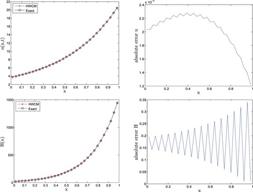
Table 7. The $L_{\mathrm{\infty }}$ errors for $\mathrm{\Delta }t=0.01$ and T = 1 at various M, Test Problem 5.6.

M	$L_{\mathrm{\infty }}(u)$	$L_{\mathrm{\infty }}(H)$	$L_{\mathrm{\infty }}(u)$	$L_{\mathrm{\infty }}(H)$	$R_c(u_M)$	$R_c(H_M)$
	$\sigma =0.01$		$\sigma =0.1$		$\sigma =0.01$
2	1.364e−1	2.099	1.347e−1	2.133	–	–
4	3.959e−2	9.665e−1	3.785e−2	1.016	1.7846	1.1189
8	1.044e−2	4.324e−1	8.670e−3	4.924e−1	1.9230	1.1604
16	2.545e−3	2.009e−1	1.024e−3	2.667e−1	2.0364	1.1059
32	4.972e−4	9.884e−2	1.367e−3	1.678e−1	2.3558	1.0233

6. Conclusion

In this article, we have implemented a Haar wavelet-based multi-resolution collocation method for the correct evaluation of the inverse Cauchy problem with an unknown source depending on space variable. The NLICP is converted into a linear PDE using a simple linearization approach. The linear PDE is then turned into a well-conditioned system of algebraic equations using Haar wavelets without using any regularization techniques. Finally, the requisite stable results against varied noise intensities are obtained by solving the full discrete system. Various forms of source terms have investigated and performed experiments using HWCM with different quantities of noise intensities. The experimental rate of convergences demonstrates that the HWCM is second-order accurate for $u(x,t)$ which is in-line with the theoretical result. From the overall comparison with exact solutions and the other method available in the literature, the HWCM is effective and performs accurately due to the well-conditional coefficient matrix.

Due to the convergence of numerical results to the exact solution and the encouraging efficiency of the HWCM, the current procedure is expendable to different types of two-dimension non-linear inverse Cauchy problems but it may be computationally expensive in three-dimensional case. The current procedure can be extended to the NLICPs with variable coefficients x and t as well as to NLICPs with separable source in the form of $F(x,t)=H(x)X(t)$. This approach can also be used to solve linear and non-linear inverse problems with time as well as space dependent piecewise source terms. These topics are the focus of our future task.

Disclosure statement

No potential conflict of interest was reported by the author(s).

References

- Liu C-S. Finding unknown heat source in a nonlinear cauchy problem by the lie-group differential algebraic equations method. Eng Anal Bound Elem. 2015;50:148–156.
- Farcas A, Lesnic D. The boundary-element method for the determination of a heat source dependent on one variable. J Eng Math. 2006;54(4):375–388.
- Berntsson F. Numerical methods for inverse heat conduction probelms [PhD thesis]. Linköping Studies in Science and Technology. Disseration No. 723, Linköping University Department of Mathematics; 2001 Dec.
- Carasso A. Determining surface temperatures from interior observations. SIAM J Appl Math. 1982;42(3):558–574.
- Eldén L. The numerical solution of a non-characteristic Cauchy problem for a parabolic equation. In: Numerical treatment of inverse problems in differential and integral equations. Springer; 1983. p. 246–268.
- Eldén L. Numerical solution of the sideways heat equation by difference approximation in time. Inverse Probl. 1995;11(4):913–923.
- Eldén L. Solving the sideways heat equation by a method of lines. ASME J Heat Transf. 1997;119:406–412.
- Eldén L, Berntsson F, Reginska T. Wavelet and fourier methods for solving the sideways heat equation. SIAM J Sci Comput. 2000;21(6):2187–2205.
- Amirfakhrian M, Arghand M, Kansa EJ. A new approximate method for an inverse time-dependent heat source problem using fundamental solutions and RBFs. Eng Anal Bound Elem. 2016;64:278–289.
- Yan L, Fu C-L, Yang F-L. The method of fundamental solutions for the inverse heat problem. Eng Anal Bound Elem. 2008;32:216–222.
- Liu C-S. Lie-group differential algebraic equations method to recover heat source in a cauchy problem with analytic continuation data. Int J Heat Mass Transf. 2014;78:538–547.
- Liu C-S, Kuo C-L, Jhao W-S. The multiple-scale polynomial trefftz method for solving inverse heat conduction problems. Int J Heat Mass Transf. 2016;95:936–943.
- Kuo C-L, Liu C-S, Chang J-R. The modified polynomial expansion method for identifying the time dependent heat source in two-dimensional heat conduction problems. Int J Heat Mass Transf. 2016;92:658–664.
- Yeih W, Liu C-S. A three-point BVP of time dependent inverse heat source problems and solving by a TSLGSM. Comput Model Eng Sci. 2009;46:107–127.
- Cannon JR. A priori estimate for continuation of the solution of the heat equation in the space variable. Annali Di Matematica Pura Ed Applicata. 1964;65(1):377–387.
- Burggraf OR. An exact solution of the inverse problem in heat conduction theory and applications. J Heat Transfer. 1964;86(3):373–380.
- Beck JV. Nonlinear estimation applied to the nonlinear inverse heat conduction problem. Int J Heat Mass Transf. 1970;3:703–716.
- Siraj-ul-Islam X, Ismail S. Meshless collocation procedures for time-dependent inverse heat problems. Int J Heat Mass Transf. 2017;113:1152–1167.
- Shidfar A, Darooghehgimofrad Z. A numerical algorithm based on RBFs for solving an inverse source problem. Bull Malays Math Sci Soc. 2016;40:1–10.
- Johansson T, Lesnic D. Determination of a spacewise dependent heat source. J Comput Appl Math. 2007;209(1):66–80.
- Liu C-S. An iterative algorithm for identifying heat source by using a DQ and a Lie-group method. Inverse Probl Sci Eng. 2015;23(1):67–92.
- Wei T, Wang J. Simultaneous determination for a space-dependent heat source and the initial data by the MFS. Eng Anal Bound Elem. 2012;36(12):1848–1855.
- Ahmadabadi M, Arab M, Ghaini F. The method of fundamental solutions for the inverse space-dependent heat source problem. Eng Anal Bound Elem. 2009;33(10):1231–1235.
- Jin Q, Wang W. Analysis of the iteratively regularized Gauss–Newton method under a heuristic rule. Inverse Probl. 2018;34(3):1–24.
- Jin Q. On a heuristic stopping rule for the regularization of inverse problems by the augmented Lagrangian method. Numerische Mathematik. 2017;136(4):973–992.
- Jin Q, Lu X. A fast nonstationary iterative method with convex penalty for inverse problems in Hilbert spaces. Inverse Probl. 2014;30(4):1–21.
- Nguyen HT, Tran TB, Vo AK, et al. On an inverse problem in the parabolic equation arising from groundwater pollution problem. Bound Value Probl. 2015;2015(1):1–23.
- Hasanov A. Identification of spacewise and time dependent source terms in 1d heat conduction equation from temperature measurement at a final time. Int J Heat Mass Transf. 2012;55(7–8):2069–2080.
- Cannon J, DuChateau P. Structural identification of an unknown source term in a heat equation. Inverse Probl. 1998;14(3):535–551.
- Siraj-ul-Islam, Ahsan M, Hussian I. A multi-resolution collocation procedure for time-dependent inverse heat problems. Int J Therm Sci. 2018;128:160–174.
- Ahsan M, Siraj-ul-Islam, Hussain I. Haar wavelets multi-resolution collocation analysis of unsteady inverse heat problems. Inverse Probl Sci Eng. 2018;27:1–23.
- Huntul M, Lesnic D. An inverse problem of finding the time-dependent thermal conductivity from boundary data. Int Commun Heat Mass Transf. 2017;85:147–154.
- Liu C-S. To recover heat source G (x)+ H (t) by using the homogenized function and solving rectangular differencing equations. Numer Heat Transf B Fundam. 2016;69(4):351–363.
- Wang F, Fan C, Hua Q, et al. Localized MFS for the inverse Cauchy problems of two-dimensional Laplace and biharmonic equations. Appl Math Comput. 2020;364:124658.
- Wang F, Hua Q, Liu C. Boundary function method for inverse geometry problem in two-dimensional anisotropic heat conduction equation. Appl Math Lett. 2018;84:130–136.
- Wang C, Wang F, Gong Y. Analysis of 2D heat conduction in nonlinear functionally graded materials using a local semi-analytical meshless method. AIMS Math. 2021;6(11):12599–12618.
- Díaz L, Martín M, Vampa V. Daubechies wavelet beam and plate finite elements. Finite Elem Anal Des. 2009;45(3):200–209.
- Liu Y, Liu Y, Cen Z. Daubechies wavelet meshless method for 2-D elastic problems. Tsinghua Sci Technol. 2008;13(5):605–608.
- Zaheer-ud-Din, Ahsan M, Ahmad M, et al. Meshless analysis of nonlocal boundary value problems in anisotropic and inhomogeneous media. Mathematics. 2020;8(11):2045.
- Siraj-ul-Islam, Aziz I, Al-Fhaid A. An improved method based on Haar wavelets for numerical solution of nonlinear integral and integro-differential equations of first and higher orders. J Comput Appl Math. 2014;260:449–469.
- Ahsan M, Ahmad I, Ahmad M, et al. A numerical Haar wavelet-finite difference hybrid method for linear and non-linear Schrödinger equation. Math Comput Simul. 2019;165:13–25.
- Liu X, Ahsan M, Ahmad M, et al. Haar wavelets multi-resolution collocation procedures for two-dimensional nonlinear Schrödinger equation. Alexandria Eng J. 2021;60(3):3057–3071.
- Nazir S, Shahzad S, Wirza R, et al. Birthmark based identification of software piracy using Haar wavelet. Math Comput Simul. 2019;166:144–154.
- Jang G-W, Kim Y, Choi K. Remesh-free shape optimization using the wavelet-galerkin method. Int J Solids Struct. 2004;41(22):6465–6483.
- Dahmen W, Kurdila A, Oswald P. Multiscale wavelet methods for partial differential equations. Vol. 6. San Diego: Academic Press; 1997.
- Maleknejad K, Mirzaee F. Using rationalized Haar wavelet for solving linear integral equations. Appl Math Comput. 2005;160(2):579–587.
- Lepik Ü. Haar wavelet method for nonlinear integro-differential equations. Appl Math Comput. 2006;176(1):324–333.
- Lepik Ü. Numerical solution of evolution equations by the Haar wavelet method. Appl Math Comput. 2007;185(1):695–704.
- Hsiao C, Wang W-J. Haar wavelet approach to nonlinear stiff systems. Math Comput Simul. 2001;57(6):347–353.
- Hsiao C. Haar wavelet approach to linear stiff systems. Math Comput Simul. 2004;64(5):561–567.
- Reddy A, Manjula S, Sateesha C, et al. Haar wavelet approach for the solution of seventh order ordinary differential equations. Math Model Eng Probl. 2016;3:108–114.
- Shah F, Abass R, Iqbal J. Numerical solution of singularly perturbed problems using Haar wavelet collocation method. Cogent Math. 2016;3(1):1202504.
- Lepik Ü, Hein H. Application of the Haar wavelet method for solution the problems of mathematical calculus. Waves Wavelets Fractals. 2015;1(1):1–16.
- Kirs M, Mikola M, Haavajõe A, et al. Haar wavelet method for vibration analysis of nanobeams. Waves Wavelets Fractals. 2016;2(1):20–28.
- Shah F, Abass R. An operational Haar wavelet collocation method for solving singularly perturbed boundary-value problems. SeMA J. 2016;74:1–18.
- Aziz I, Amin R. Numerical solution of a class of delay differential and delay partial differential equations via Haar wavelet. Appl Math Model. 2016;40(23):10286–10299.
- Aziz I, Siraj-ul-Islam, Khan F. A new method based on Haar wavelet for the numerical solution of two-dimensional nonlinear integral equations. J Comput Appl Math. 2014;272:70–80.
- Siraj-ul-Islam, Aziz I, Haq F. A comparative study of numerical integration based on Haar wavelets and hybrid functions. Comput Math Appl. 2010;59(6):2026–2036.
- Siraj-ul-Islam, Šarler B, Aziz I. Haar wavelet collocation method for the numerical solution of boundary layer fluid flow problems. Int J Therm Sci. 2011;50(5):686–697.
- Siraj-ul-islam, Aziz I, Šarler B. Wavelets collocation methods for the numerical solution of elliptic BV problems. Appl Math Model. 2013;37(3):676–694.
- Jiwari R. A Haar wavelet quasilinearization approach for numerical simulation of Burgers equation. Comput Phys Commun. 2012;183(11):2413–2423.
- Pandit S, Jiwari R, Bedi K, et al. Haar wavelets operational matrix based algorithm for computational modelling of hyperbolic type wave equations. Eng Comput (Swansea). 2017;34(8):2793–2814.
- Siraj-ul-Islam, Aziz I, Ahmad M. Numerical solution of two-dimensional elliptic PDEs with nonlocal boundary conditions. Comput Math Appl. 2015;69(3):180–205.
- Oruç Ö, Bulut F, Esen A. A Haar wavelet-finite difference hybrid method for the numerical solution of the modified Burgers equation. J Math Chem. 2015;53(7):1592–1607.
- Oruç Ö, Alaattin E, Bulut F. Numerical investigation of dynamic Euler-Bernoulli equation via 3-Scale Haar wavelet collocation method. Hacettepe J Math Stat. 2021;50(1):1–21.
- Esen A, Bulut F, Oruç Ö. A unified approach for the numerical solution of time fractional Burgers type equations. Eur Phys J Plus. 2016;131(4):1–13.
- Oruç Ö. A non-uniform Haar wavelet method for numerically solving two-dimensional convection-dominated equations and two-dimensional near singular elliptic equations. Comput Math Appl. 2019;77(7):1799–1820.
- Oruç Ö, Bulut F, Esen A. A numerical treatment based on Haar wavelets for coupled KdV equation. Int J Optim Control Theor Appl. 2017;7(2):195–204.
- Oruç Ö, Esen A, Bulut F. A Haar wavelet approximation for two-dimensional time fractional reaction–subdiffusion equation. Eng Comput. 2019;35(1):75–86.
- Oruç Ö, Bulut F, Esen A. Numerical solutions of regularized long wave equation by Haar wavelet method. Medit J Math. 2016;13(5):3235–3253.
- Pourgholi R, Tavallaie N, Foadian S. Applications of Haar basis method for solving some ill-posed inverse problems. J Math Chem. 2012;50(8):2317–2337.
- Pourgholi R, Foadian S, Esfahani A. Haar basis method to solve some inverse problems for two-dimensional parabolic and hyperbolic equations. TWMS J Appl Eng Math. 2013;3(1):10–32.
- Ahsan M, Lin S, Ahmad M, et al. A Haar wavelet-based scheme for finding the control parameter in nonlinear inverse heat conduction equation. Open Phys. 2021;19(1):722–734.
- Siraj-ul-Islam, Haq S, Ali A. A meshfree method for the numerical solution of the RLW equation. J Comput Appl Math. 2009;223(2):997–1012.
- Mokhtari R, Mohammadi M. Numerical solution of GRLW equation using Sinc-collocation method. Comput Phys Commun. 2010;181(7):1266–1274.
- Liu X, Ahsan M, Ahmad M, et al. Applications of Haar wavelet-finite difference hybrid method and its convergence for hyperbolic nonlinear Schrödinger equation with energy and mass conversionn. Energies. 2021;14(23):1–17. Available from: https://www.mdpi.com/1996–1073/14/23/7831
- Majak J, Shvartsman B, Kirs M, et al. Convergence theorem for the Haar wavelet based discretization method. Compos Struct. 2015;126:227–232.