A propos Brexit: on the breaking up of integration areas – an NEG analysis

ABSTRACT

Inspired by Brexit, the paper explores the effects of splitting an integration area or ‘Union’ on trade patterns and the spatial distribution of industry. A linear three-region New Economic Geography (NEG) model is developed and two possible situations before separation are considered: agglomeration and dispersion. By analogy with the Brexit options, soft and hard separation scenarios are considered. Firms in the leaving region may move to the larger Union market, even on the periphery, relocation substituting trade; or firms in the Union may move in the more isolated leaving region, escaping from competition. The paper also analyses deeper Union integration following separation. Instances of multistability and complex dynamics are found.

KEYWORDS:

• industry agglomeration
• trade patterns
• economic disintegration
• New Economic Geography

JEL:

• C62
• F2
• F12
• R12

INTRODUCTION

The forming of integration areas and its problems have always been at the centre of international economics. The breaking up of integration areas is far less investigated. However, with the imminent Brexit, it is precisely this breaking up and its implications that moves into the focus of interest.

Integration – not only, but in particular within the European Union (EU) – always encompasses trade as well as factor movements. This interrelationship between trade and factor movements – while neglected in the traditional international trade models – is at the core of the New Economic Geography (NEG), a paradigm pioneered by Krugman in the early 1990s (Krugman, 1991). In the following, we present an NEG analysis of the breaking up of an integration area, inspired by the Brexit.

Which stylized facts do we take on board?

• The EU is not a homogeneous integration area, but shows marked regional inequality (e.g., Eurostat, 2019a, reports that in 2017 regional gross domestic product (GDP) per capita, expressed in terms of purchasing power standards (PPS), in the richest NUTS-2 region is 20 times higher than in the poorest NUTS-2 region).¹

• With the UK, a core region is leaving the EU (Eurostat, 2019a, reports that the NUTS-1 region Greater London was one of the richest regions and enjoyed in 2017 a regional GDP per capita, expressed in terms of PPS, that was 187% of the EU average).

• Different hard and soft Brexit options are possible.

• Brexit is expected to have substantial impacts not only on trade patterns but also on factor movements, in particular on the location of firms.

• As a reaction to Brexit, the EU may try to deepen integration of the remaining regions (as Emmanuel Macron suggested in a widely noted speech; Macron, 2017).

In models of the NEG, the breaking up of an integration area is represented by an increase in trade costs. These models combine a trade model à la Krugman (1980) based upon monopolistic competition, trade costs and productive factors that choose location according to expected factor rewards. Access to a larger home market and the possibility to reach the other markets with low trade costs translates into higher factor rewards, which attracts firms to this particular location to serve the local as well as the international market. The market access effect fosters agglomeration of industry in few regions. It is mitigated by a competition effect: more firms in a location reduce factor rewards. An increase in trade costs will change the access to international markets and thus trade patterns; at the same time, the attractiveness of a region for industry location changes. NEG models focus on the long-run effects of a change in trade costs simultaneously on industry location and trade patterns.

Since Krugman’s seminal contribution (Krugman, 1991), a plethora of NEG models emerged differing in particular on the productive factor that is considered as internationally mobile and the specification of the demand function. At the core of the present study (which is inspired by the EU with its notorious low mobility of unqualified labour) is the mobility of high-qualified labour and capital; accordingly, we choose a footloose entrepreneur (FE) model. In addition, we use an FE model with a linear (instead of an isoelastic) demand function. In this model version, ‘zero trade’ situations are possible; they therefore allow one to shed a very clear light on changes in trade patterns.

Finally, we view the EU not as a homogenous integrated area, but rather as split between central and peripheral regions (indeed, with the UK leaving, part of the centre leaves the EU); and we suspect that these core–periphery (CP) patterns are not entirely exogenous, but have at least been reinforced by endogenous agglomeration processes (which are prominent in an NEG perspective). Therefore, we need a model with (at least) three regions.

Our model extends the linear NEG model put forward by Ottaviano, Tabuchi, and Thisse (2002) (more specifically, the FE version presented by Baldwin, Forslid, Martin, Ottaviano, & Robert-Nicoud, 2003), in two directions: (1) as mentioned, we increase the number of regions considered from two to three; and (2) following Behrens (2004, 2005), we study explicitly the number and direction of trade links between regions and their dependence upon the degree of trade integration.

When only two regions are considered, the possible number of trade patterns are only four (no trade, one-way trade from the first to the second region, one-way trade from the second to the first region, bilateral trade). By increasing the number of regions, the possible number of trade patterns changes substantially (even if the number of potential trade links between each pair of regions is still the same).

The specific trade pattern is determined by the size of trade costs and by the distribution of firms across the economy. In general, the market of one region is less accessible for firms of a second region, if the degree of local competition, determined by the number of home firms or of firms from a third region that have already penetrated that market (third-region effect), is higher. The existence or absence of one (or more) trade links alters substantially the attractiveness of a region and the possible long-run outcomes. Thus, in this model the evolution of the spatial distribution of firms and of trade patterns are deeply interrelated; and the long-run distribution of firms and the trade network structure are determined simultaneously.

In the literature, there are a few linear three-region NEG models that mostly assume symmetric trade costs: Castro, Correia-da-Silva, and Mossay (2012) and Gaspar, Castro, and Correia-da-Silva (2019) consider, respectively, the standard CP model and the FE model with isoelastic demand functions extended to the case of several regions larger than two, which are equally spaced along a circle. Tabuchi, Thisse, and Zeng (2005) consider an n-region economy where in each region a city emerges, that is, it is characterized by a positive share of the mobile factor (workers). The model is quite different from ours, assuming the existence of a third good (land or housing) and commuting costs. Commuting costs and land rents impact on urban costs, which are a function of the share of the mobile factor. The demand functions for the manufactured goods are linear (derived from a quadratic sub-utility function, as in Ottaviano et al., 2002), but trade costs are sufficiently low so that cities always trade with each other (i.e., the trade network is always full). Distance between the regions is equal since they are positioned on a circle and trade involves going through its centre.

Ago, Isono, and Tabuchi (2003, 2006) consider a three-region CP linear model where the regions are distributed and equally spaced along a line. They study the effect on industry location and trade patterns formation of integration as the distance between the central region and the two regions at the extremes becomes closer as the unique trade cost parameter is reduced.

Commendatore, Kubin, and Sushko (2018a, 2018b) consider a three-region FE linear model and study three simplified cases: in the first case, trade costs are so high that none of the regions is trading, no trade network structure can emerge; in the second case, trade costs between two regions are reduced allowing for trade between them, but the third region is still autarkic. Only four possible trade network configurations can emerge which are very simple. Finally, in the third case, two of the regions are sufficiently integrated that they are always engaged in bilateral trade; and trade costs between one of these regions and the third region is reduced. Also in this case only four trade network configurations are possible (differentiated by the number and direction of trade links involving the third region and the closest region belonging to the integrated area). Behrens (2011) is quite different since the author assumes a more limited factor mobility.

The present paper differs from the ones just reviewed in the following dimensions:

• We add more asymmetry by assuming a different and more general geography of trade barriers.²

• We allow for a much larger set of possible trade network structures.

• The focus is on trade disintegration (and not trade integration).

In this paper, we study the effects of an increase of the trade distance between one of the regions and the other two (more asymmetric distances and breaking of an integration area). In this sense the paper complements the previously mentioned studies.

Multiregional NEG models are notoriously complex to analyse (for a comprehensive review on multiregional NEG modelling, see Commendatore, Filoso, Kubin, & Grafeneder-Weissteiner, 2015; and also Gaspar, 2018). Many studies therefore recur to simulations. Recently, Ikeda and co-authors (e.g., Ikeda, Akamatsu, & Kono, 2012, 2017, 2018) provided some remarkable studies of multiregional geographical models in which the economies are spatially organized on a ‘racetrack’ or on a hexagonal lattice. They use group theoretic bifurcation theory in order to obtain analytical results. However, these studies are also complemented by numerical simulations (see also Barbero & Zofío, 2016). In the present paper, we primarily present simulation results complemented by intuitive explanations of the underlying economic forces.

We show that the consequences of disintegration depends upon the initial state of the integration area or ‘Union’. Accordingly, we compare two different initial states that are quintessential in an NEG perspective and that depend upon the specific interplay between local market size, local competition and trade costs. In a first scenario, the three-region economy is well integrated with small local market sizes and low trade costs; NEG models typically predict agglomeration of economic activity. In a second scenario, local market sizes are bigger and NEG models suggest an equal distribution of economic activity between the three regions. Accordingly, we choose two different values for the local market size. (Note that we deliberately abstract for exogenous differences in market size, but assume three symmetric regions; agglomerative patterns are endogenously produced by NEG forces.)

For both scenarios, we study a soft versus a hard disintegration involving different increases in trade costs between the leaving region and the regions remaining in the Union. In addition, we study the effects of a deeper integration between the regions remaining in the Union (as a reaction to the breaking up). The analysis reveals a highly complex bifurcation sequence involving many instances of coexisting long-run stationary equilibria (with complicated basins of attraction) and of cyclical and complex dynamics. Among our results, we find the following of particular interest:

• The leaving region may lose firms to the regions remaining in the Union; the firms in the Union (continue to) export, while the firms remaining in the leaving region do not (any more) – thus, firm relocation acts as substitute for trade.

• Most remarkably, the exit of one core region may induce firm relocation also to a peripheral region within the Union (which did not host industry before the breakup).

• A deepening of the integration between the remaining regions may lead to a weakening of the trade links between the Union and the leaving region; and it may put peripheral regions in danger to lose again their industry.

• In some instances, intense competition within the Union may lead to the opposite result with firms moving to the leaving region to escape the competitive pressure.³

The paper is structured as follows. The next section states the main assumptions of the model on which the analysis is based. The third section considers the short-run equilibrium, paying particular attention to the different possible trade structures. The fourth section studies the long-run implications of the model and analyses the various exiting options. The fifth section concludes.

MAIN ASSUMPTIONS

The economy is composed of three regions, labelled $R_r$ with $r=1,2,3$; two sectors: agriculture (the $A$ sector) and manufacturing or industry (the $M$ sector); two types of agents: workers ($L$, endowed with unskilled labour) and entrepreneurs ($E$, endowed with human capital). Workers are mobile across sectors but immobile across regions; entrepreneurs migrate across regions but are specific to manufacturing. The three regions share the same technology and consumer’s preferences and have the same endowment of labour, $L_1=L_2=L_3=L/3$. On purpose, we are abstracting from the fact that integration areas mostly involve regions with quite different population sizes. In this respect, the present study only represents a first attempt to shed a light on the issue of splitting of integration areas and we leave to further research the study of regions with asymmetric sizes.

The $A$ sector is perfectly competitive, constant returns prevail and production involves one unit of labour to produce one unit of the homogeneous agricultural good. In the monopolistically competitive $M$ sector, the $N$ varieties of a differentiated commodity are produced by using one entrepreneur as a fixed component. Following Ottaviano et al. (2002) and Behrens (2004, 2005), we assume that there is not a variable input requirement. This will not alter substantially the analysis. There are no economies of scope, thus, due to increasing returns, each firm produces only a variety. Following from the assumption that one entrepreneur is required to activate the production of a variety, the total number of varieties is equal to the total number of entrepreneurs, $E=N$. Denoting by ${\lambda }_r$ the share of entrepreneurs located in $R_r$, the number of varieties produced in this region corresponds to $N_r={\lambda }_{r}N={\lambda }_{r}E$.

The representative consumer’s (unskilled worker or entrepreneur) preferences are quasi-linear (Ottaviano et al., 2002), composed of a quadratic sub-utility defining the choice across the $N$ varieties of the $M$ good and a linear part for the consumption of the $A$ good: (1) $U=\alpha \sum _N^{i=1}{c}_i-\left(\frac{\text{β}-\delta }{2}\right)\sum _N^{i=1}{c}_i^2-\frac{\delta }{2}{\left(\sum _N^{i=1}{c}_i\right)}^2+C_A,$(1) where $c_i$ is the consumption of the $M$ variety $i$; and $C_A$ is the consumption of the $A$ good. The parameters are interpreted as follows: $\alpha >0$ is the intensity of preferences over the $M$ varieties; $\delta >0$ is the degree of substitutability across those varieties and the difference $\text{β}-\delta$ measures the taste for variety; and $\text{β}>\delta >0$.⁴ The budget constraint is:(2) $\sum _N^{i=1}{p}_i{c}_i+p_A{C}_A=y+p_A\overline{C_A},$(2) where $p_i$ is the price of variety $i$; $p_A$ the price of the agricultural good; $y$ is the consumer’s income; and $\overline{C_A}$ is her endowment of the agricultural good, sufficiently large to allow for positive consumption in equilibrium.

The cost of trading varieties of the $M$ good between regions, say from $R_r$ to $R_s$ (or in the opposite direction from $R_s$ to$R_r$) is $T_{rs}(=T_{sr})$; with $T_{rs}>0$ for $r\ne s$, $T_{rr}=0$ and $r,s=1,2,3$. Trade costs separate the regions introducing the spatial dimension into the economy. Different configurations are possible, for present purposes we assume that the trade distance between $R_1$ and $R_3$ and $R_2$ and $R_3$ is the same, whereas the distance between $R_1$ and $R_2$ could be shorter: $T_{13}=T_{23}=T_{EX}\ge T_{12}=T_U$. Our structure is quite different from that assumed by Ago et al. (2003, 2006) where the three regions are equally spaced along a line and one of the regions has a central position. In fact, we assume an even more asymmetric structure where the three regions are positioned on the vertices of an isosceles and acute-angled triangle. This implies that centrality is shared between two regions ($R_1$ and $R_2$) and the third region ($R_3$) is more peripheral (except in the special case $T_{EX}=T_U$). This set-up describes a three-region economy where $R_1$ and $R_2$ are part of a more integrated area, whereas $R_3$ could be less integrated with the rest of the economy. Thus, we provide a stylized set-up that can be used to describe the consequences of one of the region’s (the ‘exiting region’ $R_3$) choice to leave the integration area (the ‘Union’). We first consider the effects of an increase in $T_{EX}$ starting from the initial state $T_{EX}=T_U$. We define it as the first phase of the breaking up of the integration area. We then consider the effects of a reduction of $T_U$ when $T_{EX}>T_U$, in order to study the consequences of a second phase following the exit of $R_3$ from the Union, involving a deeper integration between the two remaining regions $R_1$ and $R_2$.

SHORT-RUN EQUILIBRIUM

In a short-run equilibrium the distribution of entrepreneurs across the regions is given. All markets are in equilibrium. We choose the $A$ good as the numeraire. From perfect competition in the $A$ sector, it follows $p_A=w=1$, where $w$ is the wage rate. To determine the short-run equilibrium solutions related to the $M$ sector, we proceed as follows. Maximizing the utility (1) subject to the constraint (2), we obtain the first order conditions for $i=1,\dots ,N$:$\frac{\mathrm{\partial }U}{\mathrm{\partial }{c}_i}=p_i\iff \frac{\mathrm{\partial }U}{\mathrm{\partial }{c}_i}-p_i=\alpha -(\text{β}-\delta )c_i-\delta \sum _N^{i=1}{c}_i-p_i=0,$from which $p_i=\alpha -(\text{β}-\delta )c_i-\delta {\mathrm{\Sigma }}_{i=1}^N{c}_i$. Solving for $c_i$, we obtain the individual linear demand function for each variety $i$:$c_i=max\left[0,a-(b+cN)p_i+cP\right],$where $P={\mathrm{\Sigma }}_{i=1}^N{p}_i$ is the price index; $a=\left(\alpha /\right(N-1)\delta +\text{β}),b=\left(1/\right(N-1)\delta +\text{β})$ and $c=\left(\delta /\right(\text{β}-\delta \left)\right[(N-1)\delta +\text{β}\left]\right)$. Moreover, we define $\widetilde{p_i}=(a+cP/b+cN)$ the cut-off price only below which the demand for variety $i$ is positive: $c_i>0$ for $p_i<{\tilde{p}}_i$.

The consumer’s demand originating from $R_s$ ($s=1,2,3$) for a $M$ good produced in $R_r$ ($r=1,2,3$), dropping the subscript $i$ because of symmetric firm behaviour (a typical assumption of NEG models), is: $c_{rs}=max[0,a-(b+cN)p_{rs}+c{P}_s]$, where $p_{rs}$ is the price of a $M$ good produced in $R_r$ and consumed in $R_s$; and:(3) $P_s=\sum _3^{k=1}{N}_k{p}_{ks}=\sum _3^{k=1}{\lambda }_{k}E{p}_{ks}$(3) is the price index in $R_s$. As before $c_{rs}>0$ if and only if $p_{rs}<{\tilde{p}}_s=(a+c{P}_s/b+cN)$. Taking into account that workers are equally spread across the regions, $L_1=L_2=L_3=L/3$, with segmented markets, the operating profit of a representative firm located in $R_r$ ($r=1,2,3$), denoted by ${\pi }_r$, is:(4) ${\pi }_r=\sum _3^{s=1}\left(p_{rs}-T_{rs}\right)q_{rs}\left(\frac{L}{3}+{\lambda }_{s}E\right).$(4) where $q_{rs}$ is the quantity produced by a firm located in region $R_r$ and brought to the market in region $R_s$. In a short-run equilibrium, demand is equal to supply in each segmented market (labelled $r,s=1,2,3$): $c_{rs}=q_{rs}$. Recalling that $N=E$ and that firms consider the price index as given, profit maximization implies:(5) $p_{rs}=\left\{\begin{array}{ccc}\frac{a+c{P}_s+T_{rs}\left(b+cE\right)}{2\left(b+cE\right)}=\frac{1}{2}\left({\tilde{p}}_s+T_{rs}\right)& \mathrm{i}\mathrm{f}& T_{rs}<{\tilde{p}}_s\\ {\tilde{p}}_s& \mathrm{i}\mathrm{f}& T_{rs}\ge {\tilde{p}}_s\end{array}\right.,$(5) which is the price that a firm located in $R_r$ quotes in the market s, with $r,s=1,2,3$ and ${\tilde{p}}_s=(a+c{P}_s/b+cE)$. Moreover, we assume $p_{rr}>0$.

Using the demand function and the price solutions, we can write:(6) $q_{rs}=\left\{\begin{array}{ccc}\left(b+cE\right)\left(p_{rs}-T_{rs}\right)& \mathrm{i}\mathrm{f}& T_{rs}<{\tilde{p}}_s\\ 0& \mathrm{i}\mathrm{f}& T_{rs}\ge {\tilde{p}}_s\end{array}\right.,$(6) which is the quantity that a firm located in $R_r$ sells in $R_s$, with $r,s=1,2,3$. According to (5) and (6), if a firm located in $R_r$ quotes in the market of $R_s$ a price larger or equal than the cut-off price ${\tilde{p}}_s$ (i.e., a price which is above the maximum reservation price consumers living in $R_s$ are prepared to pay for a positive quantity of a $M$ variety), the export from $R_r$ to $R_s$ is zero. The boundary conditions for trade, as reported in these expressions, are crucial to determine the patterns of trade between the regions, as we shall see in the analysis below.

The indirect utility for an $r$ entrepreneur is:(7) $V_r=S_r+{\pi }_r+\overline{C_A},$(7) where $S_r$ is the surplus enjoyed by an $r$ entrepreneur as a consumer:(8) $S_r=\frac{a^{2}E}{2b}+\frac{b+cE}{2}\sum _3^{s=1}{\lambda }_{s}E{p}_{sr}^2-a{P}_r-\frac{c}{2}{P}_r^2.$(8) and where the operating profit ${\pi }_r$ also represents the income of an $r$ entrepreneur.

Trade network structures

From the above discussion, the occurrence of trade between regions depends on trade costs. Above a threshold the price quoted by foreign firms is too high and exports cannot take place. It follows that the trade network structure is strongly affected by trade costs and by the spatial distribution of industry. In this subsection, we make explicit the conditions for trade between the three regions and verify that not all network structures are possible given the chosen trade costs configuration ($T_{13}=T_{23}=T_{EX}\ge T_{12}=T_U$).

Considering the three regions, $R_1$, $R_2$ and $R_3$, the existence of a trade link from one of them, labelled $R_r$, to a second one, labelled $R_s$, depends on trade costs and on competition in the local market originating both from local and foreign firms. The latter is affected by the existence or absence of another link from the third region, labelled $R_k$, to $R_s,$ with $r,s,k=1,2,3$ and $r\ne s\ne k$. If such a link is absent, $r$ firms (i.e., those located in $R_r$) only face competition from the local $s$ firms (i.e., those located in $R_s$); instead, if it is present, $r$ firms face competition also from $k$ firms (i.e., those located in $R_k$) exporting to $R_s$. In general (see expressions (5) and (6)), the condition for trade (respectively no trade) from $R_r$ to $R_s$ is:$T_{rs}<(\ge ){\tilde{p}}_s=2p_{ss}.$When trade costs are too high for a link from $R_k$ to $R_s$ ($T_{sk}\ge 2p_{ss}$), the condition for trade (no trade) from $R_r$ to $R_s$ becomes:(9) $\begin{array}{ccc}{T}_{rs}<(\ge )\frac{2a}{2b+c{\lambda }_{s}E}& \mathrm{o}\mathrm{r}& {\lambda }_s<(\ge )\frac{2\left(a-b{T}_{rs}\right)}{cE{T}_{rs}}\end{array}\mathrm{f}\mathrm{o}\mathrm{r}r,s=1,2\mathrm{a}\mathrm{n}\mathrm{d}k=3.$(9)

Moreover, since $T_{EX}\ge T_U$, for all other $r$, $s$ and $k$ a link from $R_r$ to $R_s$ cannot occur. When such a link does not exist the price quoted by $s$ firms in the local market is:$p_{ss}=\frac{a}{2b+c{\lambda }_{s}E}.$Instead, when it exists, the local price in $R_s$ is:$p_{ss}=\frac{a+\left(T_{rs}/2\right)c{\lambda }_{r}E}{2b+c\left({\lambda }_r+{\lambda }_s\right)E}.$

When trade costs allow for a link from $R_k$ to $R_s$ ($T_{sk}<2p_{ss}$), the condition for trade (no trade) from $R_r$ to $R_s$ becomes:(10) $\begin{array}{r}{T}_{rs}<(\ge )\frac{2a+cE{\lambda }_k{T}_{sk}}{2b+c\left({\lambda }_s+{\lambda }_k\right)E}\mathrm{o}\mathrm{r}\\ & {\lambda }_s<(\ge )\frac{2\left(a-b{T}_{rs}\right)}{cE{T}_{rs}}+\frac{T_{sk}-T_{rs}}{T_{rs}}{\lambda }_k\mathrm{f}\mathrm{o}\mathrm{r}r=3\mathrm{a}\mathrm{n}\mathrm{d}s,k=1,2.\end{array}$(10) Moreover, since $T_{EX}\ge T_U$, for all other $r$, $s$ and $k$ a link from $R_r$ to $R_s$ always occur. When such a link does not exist the price fixed locally by $s$ firms is:$p_{ss}=\frac{a+\left(T_{sk}/2\right)c{\lambda }_{k}E}{2b+c\left({\lambda }_s+{\lambda }_k\right)E}.$Instead, when it exists, the local price in $R_s$ is:$p_{ss}=\frac{a+\left(\left(T_{rs}/2\right){\lambda }_r+\left(T_{sk}/2\right){\lambda }_k\right)cE}{2b+cE}.$From (10), it follows that the condition for trade (no trade) from $R_r$ and $R_s$ is less (more) stringent, the smaller are ${\lambda }_s$, ${\lambda }_k$ (therefore, the larger is ${\lambda }_r$) and $T_{rs}$ and the larger is $T_{sk}$. That is, trade (no trade) from $R_r$ to $R_s$ is more (less) likely the less competitive is the market in $R_s$ (where now the degree of competition is also determined by the number of $k$ firms selling in that market), the closer are regions $R_r$ and $R_s$ and the farther away are regions $R_s$ and $R_k$.

Combining conditions (9) and (10) (as shown in Commendatore, Kubin, & Sushko, 2018c), the possible trade network structures ($NS$) are numbered 18 (Figure 1), grouped into 10 types (which are isomorphic) and named according to the terminology of social network analysis (SNA).⁵

Figure 1. Trade network structures.

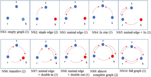
According to Figure 1, when the network structure $NS1$ (empty graph, in the terminology of SNA) prevails, there are zero trade links (full autarky case); there is only one trade link in the two network structures $NS2$ (single edge) ($NS21$, $NS22$): one-way (or unilateral) trade from $R_r$ to $R_s$, where $r,s=1,2$ and $r\ne s$; in the network structure $NS3$ (mutual edge), there are two trade links corresponding to two-way (or bilateral) trade between $R_1$ and $R_2$; when one of the three network structures $NS4$ (in star) ($NS41$, $NS42$, $NS43$) prevails, there are two links involving all three regions: one-way trade from $R_r$ to $R_s$ and from $R_k$ to $R_s$, where $r,s,k=1,2,3$ and $r\ne s\ne k$; in the two network structures $NS5$ (mutual edge + in) ($NS51$, $NS52$) there are three links: two-way trade between $R_r$ and $R_s$ and one-way trade from $R_k$ to $R_r$, where $r,s=1,2$, $k=3$ and $r\ne s$; we have three links also in the two networks structures $NS6$ (transitive) ($NS61$, $NS62$): one-way trade from $R_r$ to $R_s$, $R_r$ to $R_k$ and $R_s$ to $R_k$, where $r,s=1,2$, $k=3$ and $r\ne s$; there are four trade links when one of the three network structures $NS7$ (mutual edge + double in) ($NS71$, $NS72$, $NS73$) prevails: one-way trade from $R_r$ to $R_s$ and from $R_r$ to $R_k$ and bilateral trade between $R_s$ and $R_k$, where $r,s,k=1,2,3$ and $r\ne s\ne k$; also four links exist in the network structure $NS8$ (mutual edge + double out): two-way trade between $R_1$ and $R_2$, one-way trade from $R_1$ to $R_3$ and from $R_2$ to $R_3$; five links characterize the two network structures $NS9$ (almost complete graph) ($NS91$, $NS92$): two-way trade between $R_r$ and $R_s$ and $R_s$ and $R_k$ and one-way trade from $R_r$ to $R_k$, where $r,s=1,2$, $k=3$ and $r\ne s$; finally, when the network structure $NS10$ (complete graph) prevails, all regions are engaged in mutual trade.

Note that in the special case $T_U=T_E$, only trade network structures symmetric with respect to all three regions (i.e., with a symmetric number of links or with several isomorphic cases equal to three) can exist. These structures are only eight, grouped into four isomorphic cases ($NS1$, $NS41$, $NS42$, $NS43$, $NS71$, $NS72$, $NS73$, $NS10$).

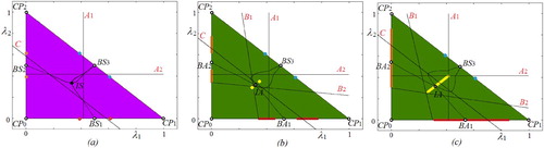
Short-run solutions

To each trade network configuration – which depends on trade costs and the spatial distribution of entrepreneurs – corresponds a different set of short-run solutions. We cannot present here the whole set of solutions (but see Commendatore et al., 2018c). Figure 2 presents examples of possible combinations of trade costs giving rise to different trade network configurations. Here the combinations of ${\lambda }_1$ and ${\lambda }_2$ (after taking into account that ${\lambda }_3=1-{\lambda }_1-{\lambda }_2$) that allow for a specific network configuration are represented by areas of the same colour. The lines $A_1$, $A_2$ and $C$ correspond to the conditions in (9), that is, there is not an incoming trade link from a third region affecting the existence of a link between two regions; and the lines $B_1$ and $B_2$ correspond to the conditions in (10), that is, such an incoming link exists (however, notice that when $T_U=T_{EX}$, the two sets of conditions are identical). The lines are given as:(11) $\begin{array}{cc}{A}_1:\left\{({\lambda }_1,{\lambda }_2):{\lambda }_1=\tilde{\lambda }\right\};& A_2:\left\{({\lambda }_1,{\lambda }_2):{\lambda }_2=\tilde{\lambda }\right\};\\ B_1:\left\{({\lambda }_1,{\lambda }_2):{\lambda }_1=\overline{\lambda }-\theta {\lambda }_2\right\};& B_2:\left\{({\lambda }_1,{\lambda }_2):{\lambda }_2=\overline{\lambda }-\theta {\lambda }_1\right\};\\ C:\left\{({\lambda }_1,{\lambda }_2):{\lambda }_1=1-\overline{\lambda }-{\lambda }_2\right\};& \end{array}$(11) where:$\overline{\lambda }=\frac{2(a-b{T}_{EX})}{cE{T}_{EX}},\tilde{\lambda }=\frac{2(a-b{T}_U)}{cE{T}_U}\mathrm{a}\mathrm{n}\mathrm{d}\theta =\frac{T_{EX}-T_U}{T_{EX}}.$

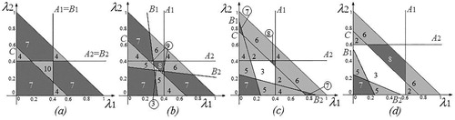
Figure 2. Examples of possible configurations of trade costs giving rise to different trade network configurations. Here $a=b=c=1/3$, $E=10$ and $T_U=T_{EX}=0.325$ in (a); $T_U=0.325$ and $T_{EX}=0.37$ in (b); $T_U=0.325$ and $T_{EX}=0.45$ in (c); and $T_U=0.25$ and $T_{EX}=0.45$ in (d).

The lines $A_1$ and $A_2$ only involve $R_1$ and $R_2$; instead, the lines $B_1$, $B_2$ and $C$ also involve $R_3$. Moreover, trade is allowed (not allowed) on the left (right) of $A_1$ and $B_1$, below (above) $A_2$ and $B_2$ and above (below) $C$.⁶ Therefore, the crossing of these borders determine changes in the trade network structure.

We now look more in detail Figure 2, where the different panels involve different trade costs combinations and show the corresponding trade network configurations (a number $x$ in an area indicates the trade network structure $NSx)$. These trade costs combinations are chosen in order that some trade always occur. In Figure 2(a), $T_U=T_{EX}$, only symmetric trade network structures exist ($NS4$, $NS7$ and $NS10$). By increasing $T_{EX}$, a larger variety of trade network structures become possible ($NS3$, $NS4$, $NS5$, $NS6$, $NS7$, $NS8$ and $NS9$), which also involve more asymmetric structures, that is, $NS5$, $NS6$ and $NS8$ (notice, however, that symmetry between regions $R_1$ and $R_2$ is kept). Given the longer distance between the Union and the exiting region, $NS10$ cannot occur anymore substituted by less connected trade network structures ($NS3,NS8$ and $NS9$). Similarly, the areas corresponding to trade networks $NS7$ shrunk, replaced by the less connected network structures $NS5$ and $NS6$. By increasing further $T_{EX}$, as in Figure 2(c), this pattern – less connected network structures substituting more connected ones – is confirmed as the $NS7$ and $NS8$ areas shrink and the $NS6$ and $NS3$ areas expand. This is also emphasized by the emergence of the $NS2$ areas that replace points belonging to $NS4$, $NS6$ and $NS7$ areas.⁷ Finally, Figure 2(d) considers a strong reduction of $T_U$ keeping $T_{EX}$, as in Figure 2(c). We notice that the $NS3$ and $NS8$ areas expand substantially, a consequence of the closer distance between $R_1$ and $R_2$; and that there is only one $NS7$ area corresponding to the case of bilateral trade between $R_1$ and $R_2$ and one-way trade from $R_3$ to $R_1$ and from $R_3$ to $R_2$ ($NS73$), the other two replaced by points belonging to $NS6$ areas (i.e., by $NS61$ or $NS621$, with the loss of a trade link from $R_3$ to $R_1$ or from $R_3$ to $R_2$).

Finally, note that the borders and vertices of the triangles in Figure 2 represent special cases. On each border firms are located in only two regions, whereas the third region is empty, and on a vertex (the crossing of two borders) all industry is agglomerated in one region. Therefore, some of the outward links (involving exporting firms) that may occur in a neighbourhood of a point on a border or of a vertex (where all the industry shares are positive) are necessarily absent in those points without industry.

DYNAMICS

In the long run, entrepreneurs are free to move across the regions. The migration hypothesis – which is framed in discrete time – is based on the idea that entrepreneurs move in another region, if they can enjoy in the new location a higher indirect utility. Taking into account that ${\lambda }_3=1-{\lambda }_1-{\lambda }_2$, the indirect utilities can be expressed as functions of the shares of entrepreneurs located in $R_1$ and $R_2$, that is, $V_r({\lambda }_1,{\lambda }_2)$, $r=1,2,3$. The following equation is at the centre of the migration law:(12) $F_r\left({\lambda }_1,{\lambda }_2\right)={\lambda }_r\left(1+\gamma {\mathrm{\Omega }}_r\left({\lambda }_1,{\lambda }_2\right)\right)$(12) where:${\mathrm{\Omega }}_r({\lambda }_1,{\lambda }_2)=\frac{V_r({\lambda }_1,{\lambda }_2)-\left[{\lambda }_1{V}_1\right({\lambda }_1,{\lambda }_2)+{\lambda }_2{V}_2({\lambda }_1,{\lambda }_2)+(1-{\lambda }_1-{\lambda }_2\left)V_3\right({\lambda }_1,{\lambda }_2\left)\right]}{{\lambda }_1{V}_1({\lambda }_1,{\lambda }_2)+{\lambda }_2{V}_2({\lambda }_1,{\lambda }_2)+(1-{\lambda }_1-{\lambda }_2)V_3({\lambda }_1,{\lambda }_2)}.$According to (12) – which resembles the replicator dynamics – entrepreneurial migration depends on the difference between the indirect utility enjoyed in region $R_r$ (see equation 7) and the weighted average of the indirect utilities in all three regions. The parameter $\gamma >0$ represents the migration speed.

Taking into account the obvious constraint on the shares (i.e., they must belong to the interval [0, 1]), the change in the spatial distribution of entrepreneurs (from a short-run allocation $({\lambda }_1,{\lambda }_2)$ to the next one $\left(Z_1\right({\lambda }_1,{\lambda }_2),Z_2({\lambda }_1,{\lambda }_2\left)\right)$), can be described by a two-dimensional (2D) piecewise smooth map $Z:{\mathbb{R}}^2\to {\mathbb{R}}^2$ defined as follows:(13) $Z:\left({\lambda }_1,{\lambda }_2\right)\mapsto \left(Z_1\left({\lambda }_1,{\lambda }_2\right),Z_2\left({\lambda }_1,{\lambda }_2\right)\right),$(13) where:$Z_r({\lambda }_1,{\lambda }_2)=\left\{\begin{array}{ccccc}0& \mathrm{i}\mathrm{f}& F_r\le 0,& & \\ F_r& \mathrm{i}\mathrm{f}& F_r>0,& F_s>0,& F_r+F_s<1,\\ \frac{F_r}{F_r+F_s}& \mathrm{i}\mathrm{f}& F_r>0,& F_s>0,& F_r+F_s\ge 1,\\ \frac{F_r}{1-F_s}& \mathrm{i}\mathrm{f}& F_r>0,& F_s\le 0,& F_r+F_s<1,\\ 1& \mathrm{i}\mathrm{f}& F_r>0,& F_s\le 0,& F_r+F_s\ge 1,\end{array}\right.$with $r=1,s=2$ for $Z_1\left({\lambda }_1,{\lambda }_2\right)$ and $r=2,s=1$ for $Z_2\left({\lambda }_1,{\lambda }_2\right)$.

The following properties of map $Z$, which are useful to identify its fixed points (corresponding to the stationary long-run equilibria of the model), follow from its definition:

• Property 1. In the $({\lambda }_1,{\lambda }_2)$-phase plane, any trajectory of map $Z$ is trapped in a triangle denoted $S$, whose sides or borders $I_{bi},$ $i=1,2,3,$ are invariant lines of map $Z$:(14) $I_{b1}=\left\{\left({\lambda }_1,{\lambda }_2\right):{\lambda }_2=0\right\},I_{b2}=\left\{\left({\lambda }_1,{\lambda }_2\right):{\lambda }_1=0\right\},I_{b3}=\left\{\left({\lambda }_1,{\lambda }_2\right):{\lambda }_2=1-{\lambda }_1\right\}.$(14)

• Property 2. $Z$ is symmetric with respect to the diagonal $D=\left\{\left({\lambda }_1,{\lambda }_2\right):{\lambda }_1={\lambda }_2\right\}$, which is invariant for $Z$.⁸

• Property 3. The vertices of $S$ are core–periphery ($CP$) fixed points:(15) $C{P}_0:({\lambda }_1,{\lambda }_2)=(0,0),C{P}_1:({\lambda }_1,{\lambda }_2)=(1,0),C{P}_2:({\lambda }_1,{\lambda }_2)=(0,1),$(15) corresponding to full agglomeration of the industrial activity, with all the entrepreneurs located in only one region.

• Property 4. Any interior fixed point of $Z$, if it exists, is given by intersection of the curves:(16) ${\mathrm{\Omega }}_1=\left\{\left({\lambda }_1,{\lambda }_2\right):{\mathrm{\Omega }}_1\left({\lambda }_1,{\lambda }_2\right)=0\right\}\mathrm{a}\mathrm{n}\mathrm{d}{\mathrm{\Omega }}_2=\left\{\left({\lambda }_1,{\lambda }_2\right):{\mathrm{\Omega }}_2\left({\lambda }_1,{\lambda }_2\right)=0\right\}.$(16) An interior equilibrium is characterized by positive shares of entrepreneurs in all regions.

• Property 5. Any border fixed point belonging to $I_{bi},$ $i=1,2,$ if it exists, is an intersection point of ${\mathrm{\Omega }}_i$ and $I_{bi},$ while any border fixed point belonging to $I_{b3}$ is an intersection point of ${\mathrm{\Omega }}_1,$ ${\mathrm{\Omega }}_2$ and $I_{b3}$. A border equilibrium is characterized by positive shares of entrepreneurs in two regions and no entrepreneurs in the third one.

We denote an interior symmetric fixed point by $IS:$ $({\lambda }_1,{\lambda }_2)=(1/3,1/3)\in D,$ and an interior asymmetric fixed point by $IA:$ $({\lambda }_1,{\lambda }_2)=({\lambda }_{IA},{\lambda }_{IA})\in D$, with ${\lambda }_{IA}\ne 1/3$. The border symmetric / asymmetric fixed points are denoted by $B{S}_i/B{A}_i\in I_{bi}$, $i=1,2,3$. In case of coexisting fixed points of the same type, we use additional labels. Note that a border symmetric equilibrium is such that, when positive, the two shares are equal to 0.5. For $T_{EX}\ne T_U$, map $Z$ has only one border symmetric equilibrium, $B{S}_3:({\lambda }_1,{\lambda }_2)=(1/2,1/2)\in I_{b3}$.

Besides the borders $I_{bi}$ of the triangle $S,$ map $Z$ changes its definition along five more borders (which, depending on the parameters, may or may not intersect the triangle $S$) that are given in (11), and the crossing of which determine a change in the network structure.

To investigate how the dynamics of map $Z$ depends on the parameters $T_{EX}$, $T_U$ and $L$, we fix in our simulations:(17) $a=b=c=\frac{1}{3},\overline{C_A}=1,\gamma =10,E=10$(17) and consider first the bifurcation structure of the $(T_{EX},L)$ parameter plane for $T_U=0.325$, then of the $(T_{EX},T_U)$ parameter plane for $L=20$.

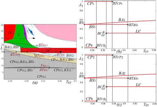
Figure 3(a) presents a 2D bifurcation diagram in the $(T_{EX},L)$ parameter plane for $T_U=0.325$. It summarizes all possible long-term dynamic behaviour involving map $Z$. To produce this 2D bifurcation diagram, we started by using only one initial condition (one initial distribution of entrepreneurs across space) identifying within the $(T_{EX},L)$ parameter plane all the attractors for that given initial condition. After running several simulations, we discovered within the same $(T_{EX},L)$ parameter plane other attractors corresponding to different initial conditions. The coexistence of more than one attractor, that is, a long-run state of the industrial distribution of the economic activity across space, is a typical result of NEG models that, in our context, is strengthened by the increase in the number of regions. The presence of different attractors (each with a different basin of attraction, i.e., the set of initial conditions that converge to that attractor) may lead to different long-run outcomes depending on the initial distribution of entrepreneurs. In order to highlight this finding, Figure 3(a) also indicates these coexisting attractors. In particular, the region denoted by $C{P}_{012}$ is related to coexisting attracting CP fixed points $C{P}_0$, $C{P}_1$, $C{P}_2;$ the regions $B{A}_{12}$ and $B{S}_3$ to the border fixed points $B{A}_1,$ $B{A}_2$ and $B{S}_3$, respectively; the regions denoted by $IA$ and $I{A}^{\mathrm{\prime }}$ (shown in red)⁹ is related to one (or two coexisting) attracting interior fixed point(s); the regions denoted by two, three and four (shown in green, light blue and magenta) are associated with attracting two-, three- and four-cycle, respectively; the region denoted by $M$ (shown in pink) corresponds either to a so-called Milnor attractor¹⁰ on the border $I_{b3}$ or to the M-attracting¹¹ fixed points $C{P}_1$ and $C{P}_2$. All regions are separated by boundaries related to various bifurcations at which the stability properties, the number or the qualitative properties of attractors (stationary equilibria, of higher periodicity or even chaotic) may change.¹² The one-dimensional (1D) bifurcation diagrams in Figure 3(b) and (c), plotting, respectively, ${\lambda }_1$ and ${\lambda }_2$ versus $T_{EX}$ for $L=20$ (see the horizontal arrow in Figure 3(a)) illustrates these coexisting attractors. It shows only the (stable) fixed points; the grey vertical lines help to visualize the different borders (which are also present in Figure 3(a)) crossing which a specific fixed point loses stability or disappears (below we discuss the different types of bifurcations induced by the presence of borders): for example, for $T_{EX}<B{T}_{CP0}$ six – locally stable – fixed points coexist, namely three CP fixed points $C{P}_0$, $C{P}_1$, $C{P}_2$; two asymmetric border fixed points $B{A}_1$ and $B{A}_2$; and one border symmetric fixed point $B{S}_3$. At $T_{EX}=B{T}_{CP0}$, $C{P}_0$ loses stability via a Border transcritical bifurcation; and the number of coexisting fixed point is reduced to five. Each coexisting fixed point has a specific basin of attraction. Examples of attractors and their basins are presented in Figures 4, 5 and 8, where attracting, repelling and saddle fixed points are marked by black, white and grey circles, respectively; the curves ${\mathrm{\Omega }}_i$, $i=1,2,$ given in (16), as well as the border lines $A_i,$ $B_i$ and $C$ defined in (11) are also shown.

Figure 3. (a) Bifurcation structure of the $(T_{EX},L)$ parameter plane of map $Z$ at $T_U=0.325$; (b, c) corresponding one-dimensional bifurcation diagrams of ${\lambda }_1$ and ${\lambda }_2$ versus $T_{EX}$ plotted for $L=20$ and $0.325<T_{EX}<0.46$ (see the arrow indicated in (a) in correspondence of that value of $L$) presenting only the stable fixed points. All the other parameters are fixed as in (17).

Splitting of the integration area: phase 1

In this subsection, we study the consequences of one of the regions, $R_3$, separating from the other two, $R_1$and $R_2$. This corresponds to an increase in $T_{EX}$ for a given $T_U$. As an NEG perspective suggests (e.g., Baldwin et al., 2003), two are the most likely prior scenarios, depending on the interplay between trade costs, local competition and local demand. In the first scenario, the immobile component of demand, $L$, is not too large compared with the mobile component, $E$ (i.e., we set $L=20$, which is only twice $E=10$); the economy is well integrated and NEG models typically predict agglomeration of economic activity. In the second scenario, local market sizes are bigger (we set $L=30$, which is three times $E=10$) and NEG models suggest an equal distribution of economic activity.¹³ In the following, we first describe how stability properties of equilibria and dynamics are affected by changing the relevant parameters; and then we provide an economic interpretation of the results.

Starting from the first scenario, we fix $L=20$ and increase $T_{EX}$ beginning from $T_{EX}=T_U=0.325$. As shown in Figure 4(a), for such parameter values there are six coexisting attracting fixed points: the CP equilibria $C{P}_0,$ $C{P}_1,$ and $C{P}_2$ and the symmetric border equilibria $B{S}_1,$ $B{S}_2$ and $B{S}_3$. The basins of attraction of the CP equilibria (coloured differently, respectively in red, blue and green) are relatively small, whereas those of the symmetric border equilibria (coloured differently, respectively in brown, light blue and Ceylon yellow) are relatively large. By increasing $T_{EX}$ at first $C{P}_0$ loses stability and the attracting fixed points are reduced to five: $C{P}_1$, $C{P}_2$, $B{A}_1$, $B{A}_2$ and $B{S}_3$ (Figure 4(b), where $T_{EX}=0.35$; note also that $B{A}_1$ and $B{A}_2$ are now only symmetric with respect to each other). Increasing further $T_{EX}$ the interior asymmetric fixed point $I{A}^{\mathrm{\prime }}$ (Figure 4(b)) hits the border $B$ (i.e., the intersection of the lines $B_1$ and $B_2$ in Figure 4; see also Figure 3(a)) and gains stability. For a larger $T_{EX}$ also $C{P}_1$ and $C{P}_2$ lose stability and after this sequence of bifurcations map $Z$ has four coexisting attracting fixed points: $B{A}_1,$ $B{A}_2$, $B{S}_3$ and $I{A}^{\mathrm{\prime }}$ (Figure 4(c), where $T_{EX}=0.38$). Finally, by further increasing $T_{EX}$, also the fixed point $B{S}_3$ loses its stability merging with the unstable fixed point $IA$ so that only three attractors are left: the fixed points $B{A}_1,$ $B{A}_2$ and $I{A}^{\mathrm{\prime }}$ (Figure 4(d), where $T_{EX}=0.45$).¹⁴

Figure 4. Basins of coexisting attracting fixed points of map $Z$ for $T_U=0.325,$ $L=20$ and $T_{EX}=0.325$ in (a); $T_{EX}=0.35$ in (b); $T_{EX}=0.38$ in (c); and $T_{EX}=0.45$ in (d). The related parameter points are marked in Figure 3(a) by black circles along the arrowed line drawn at $L=20$. The other parameters are fixed as in (17).

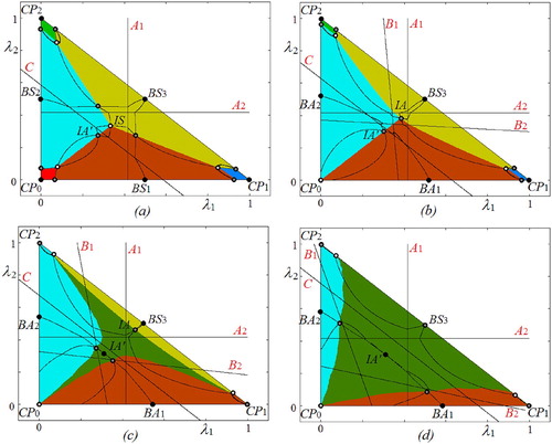
In Figure 4(a) we have chosen parameter values according to the first scenario mentioned above: the interior symmetric fixed point, $IS$, is unstable and the possible constellations of equilibria prior the splitting of the integration area involve full or partial agglomeration. Figure 2(a) allows one to determine the respective trade patterns. The consequences of a soft separation (involving a small change of $T_{EX}$) on industry location can be seen by comparing Figure 4(a) with (b); comparing Figure 4(a) with (d) reveals the consequences of a hard separation (involving a large change of $T_{EX}$) on industry location; the corresponding trade patterns are found in Figure 2(c):

• First consider the situation before separation where industry is agglomerated in only one region, that is, one of the CP fixed points $C{P}_0,$ $C{P}_1,$ $C{P}_2$ in Figure 4(a) prevails. The trade structure is of the $NS7$ type, that is, the industrialized core exports to both peripheral regions (whose reciprocal trade cannot occur since industry is absent). If the core was in the Union (i.e., in $C{P}_1$ or $C{P}_2$), this state may continue after a mild separation (analogous to the soft Brexit scenario), as shown in Figure 4(b), but notice the smaller basins of attraction of $C{P}_1$ and $C{P}_2$. With a sufficiently big shock or if the core was in $C{P}_0$, that is, located in the leaving region $R_3$, $B{A}_1$ or $B{A}_2$ will be the long-run outcome: some firms leave the industrialized core and move to one of the other regions, although it is now more distant (because of the higher trade costs), in order to gain market access. In fact, firms’ relocation replaces the export link and the trade pattern changes to the $NS4$ type; the former core region and the newly industrialized region export to the remaining peripheral region. Figure 4(d) shows the situation after a substantial separation (as in a hard Brexit scenario). If the core was located in the Union (in $C{P}_1$ or $C{P}_2$) and in the absence of large shocks (notice the smaller basins of attraction of $B{A}_1$ and $B{A}_2$), the long-run configuration that we have just discussed also applies in this case of a hard separation. However, if the shocks are large or if the core was located in the leaving region $R_3$, a hard separation may induce firms, that leave the industrialized core, to move to both other regions. The equilibrium will be $I{A}^{\mathrm{\prime }}$, and the trade pattern changes to the $NS3$ type, where only the two regions in the Union trade with each other. If the core was in region $R_3$, firm relocation (following market access) substitutes export links (that now involve higher trade costs) and $R_3$ changes from being the only exporting region to autarkic region. Interestingly, if the core was in the Union, firm relocation to the peripheral region within the Union does not destroy the trade link (that has unchanged trade costs).

• Alternatively, consider a situation before separation where industry is partly agglomerated in two regions, that is, one of the symmetric border equilibria $B{S}_1,$ $B{S}_2$ and $B{S}_3$ prevails (Figure 4(a)). The trade network is of type $NS4$ and involves only exports from the two industrialized towards the peripheral region. If $R_3$ is one of the industrialized region, a soft separation (Figure 4(b)) induces some $R_3$ firms to move to the Union’s industrialized region (in order to gain market access). Thus, the border equilibria $B{A}_1$ and $B{A}_2$ become increasingly asymmetric; in addition, their basin of attraction increases. The same applies in the case of a hard separation (Figure 4(d)), but now $B{A}_1$ and $B{A}_2$ have a reduced basin of attraction. Instead, if industry was only located within the Union, a soft separation does not induce firm relocation and $B{S}_3$ prevails (Figure 4(b)), though it has a smaller basin of attraction. In all these cases, trade patterns continue to be of the $NS4$ type. With large shocks or if industry was only located within the Union, a hard separation (Figure 4(d)) will push the economy to $I{A}^{\mathrm{\prime }}$ and some firms will move from the two industrialized regions to the periphery. Note that firm relocations destroy again export links between the Union and the leaving region (that involve increased trade costs) and trade networks are of the $NS3$ type. The incentives for firm relocation are worth noticing. If industry was located only within the Union, after a hard separation some firms leave the Union in order to locate in $R_3$, where they find less competition. The larger $T_{EX}$ the stronger this incentive becomes. If instead the peripheral region was in the Union, it attracts industry both from the leaving region $R_3$ because it provides access to the Union market, and from the Union’s industrialized region, because the overall market is now smaller (since $R_3$ is more difficult to be reached and has less firms) and it is no longer sufficient to sustain agglomeration within the Union.

To sum up: before the splitting, the Union was well integrated and – corresponding to an NEG logic – agglomeration in one or two regions was a very likely outcome. With a soft separation, CP outcomes become less likely, as well as agglomeration in the two regions in the Union. With a hard separation, the equilibrium $I{A}^{\mathrm{\prime }}$, in which industry is located in all three regions, becomes more likely. Thus, with a hard separation, peripheral regions that did not have industry can attract firms. Note that only the two regions in the Union trade, whereas $R_3$ becomes autarkic.

Considering the second scenario before the splitting of the integration area, we assume $L=30$. In this scenario, markets are larger and trade costs are not sufficiently low to make the Union a well-integrated area. NEG models predict dispersion of economic activity. Indeed, Figure 5(a) illustrates that for $T_{EX}=T_U=0.325$, the map $Z$ has a unique attractor, which is the interior symmetric fixed point $IS$.¹⁵ Figure 3(a) shows that when $L$ is sufficiently large, the bifurcation structure becomes quite complicated involving attracting cycles of different periods (given that the value of $\gamma$ is sufficiently large).

Figure 5. Attractors of map $Z$ for $T_U=0.325,$ $L=30$ and $T_{EX}=0.325$ in (a); $T_{EX}=0.37$ in (b); and $T_{EX}=0.4$ in (c). The other parameters are fixed as in (17).

Interestingly, separation, that is, increasing $T_{EX}$, does not destroy the symmetry between the two regions remaining in the Union, that is, ${\lambda }_1={\lambda }_2={\lambda }_D$ holds along the long-period attractor. We exploit this property and focus on the dynamics of the 1D map, which is a restriction of map $Z$ to the diagonal. This will allow for a neater description of the bifurcation sequence occurring by increasing $T_{EX}$. These bifurcations – illustrated in the 1D bifurcation diagram of ${\lambda }_1$ versus $T_{EX}$ for ${\lambda }_1={\lambda }_2$ and $T_U<T_{EX}<0.4$ presented in Figure 6 – affect not only industry location but also trade patterns (which can be determined using the lines $A$, $B$ and $C$, which correspond, respectively, to the intersections between the lines $A_1$ and $A_2$, $B_1$ and $B_2$ and the line $C$ and the diagonal line).

Figure 6. One-dimensional (1D) bifurcation diagram ${\lambda }_1$ versus $T_{EX}$ of a 1D map which is a restriction of map $Z$ to the diagonal ${\lambda }_1={\lambda }_2$; here $L=30$ and $T_U<T_{EX}<0.4$ (see the horizontal arrow drawn at $L=30$ in Figure 3(a)). All the other parameters are fixed as in (17).

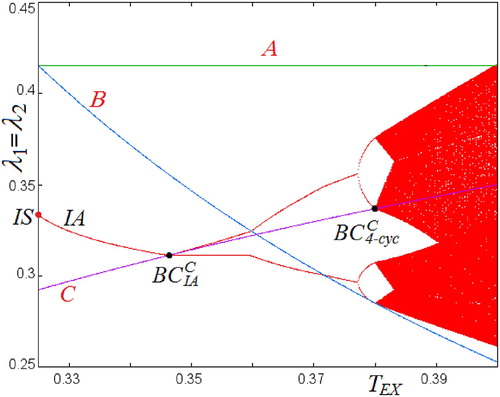
As one can see in Figure 6, with a moderate increase in $T_{EX}$, the interior fixed point $IA$ remains stable. Such a soft separation increases the incentive for firms to leave the Union and to move to region $R_3$ (where they are sheltered from competition). In the situation before separation and for a moderated increase in $T_{EX}$, ${\lambda }_D$ lies between the $B$ and $C$ lines; this corresponds to $NS10$ and we observe a full trade network.

When $IA$ collides with the border $C$, a bifurcation occurs,¹⁶ after which $IA$ has lost stability and the economy fluctuates between two points, corresponding to the dark dots (in the printed version of the paper) or to the yellow dots (in the online version of the paper) close to $IA$ in Figure 5(b), which still belong to the diagonal (Figure 5(b), where $T_{EX}=0.37$). That is, the unique attractor of $Z$ is a cycle of period 2 (or two-cycle). We denote these two points belonging to the two-cycle by ${\lambda }_{D0}$ and ${\lambda }_{D1}$, with ${\lambda }_{D0}>{\lambda }_{D1}.$ ${\lambda }_{D0}$ continues to lie in $NS10$, whereas ${\lambda }_{D1}$ lies below the $C$ line in the $NS7$ area: the Union’s regions $R_1$ and $R_2$ trade with each other and $R_3$ exports to them; however, the regions in the Union do not export to $R_3$, since a low ${\lambda }_{D1}$ translates into a high number of firms in $R_3$ and to an intense competition. Then this cycle of period 2 collides with the border $B$. This collision does not lead to a qualitative change in the industry location (i.e., a persistence border collision occurs); trade patterns, however, do change. First, ${\lambda }_{D0}$ crosses the $B$ line and enters the area corresponding to $NS8$. The regions in the Union $R_1$ and $R_2$ are still trading with each other. Given the high value of ${\lambda }_{D0}$ and the corresponding high (low) number of firms in the Union ($R_3$), competition is high in the regions in the Union, but low in $R_3$; exporting to $R_3$ is attractive for firms located in regions in the Union, but exporting to the Union is not attractive for firms in $R_3$. ${\lambda }_{D1}$ continues to involve $NS7$. Next change in the trade pattern occurs when ${\lambda }_{D1}$ crosses the $B$ line and enters the area corresponding to $NS3$, implying that region $R_3$ is autarkic and does not trade at all – given $T_{EX}$, ${\lambda }_{D1}$ is in an intermediate range where there is no incentive for trade between $R_3$ and regions in the Union. The latter continue to trade with each other and ${\lambda }_{D0}$ remains in the area associated with $NS8$. Thus, over the cycle of period 2, which involves a switch between a high and a low number of firms within the Union, $R_1$and $R_2$ always trade with each other; they export to $R_3$ only in every other period, that is, in the period in which the number of firms (and thus competition) is low in $R_3$. However, the pattern of exports from $R_3$ to the Union’s regions changes markedly. Initially, $R_3$ always exports to the regions in the Union; then, only in every other period, that is, in periods in which the number of firms (and thus competition) in the regions in the Union is low (and in $R_3$ is high); and finally, they never export.

Further increasing $T_{EX}$ leads to a (flip) bifurcation of the two-cycle into an attracting cycle of period 4, a four-cycle: the economy fluctuates between four points, with now two of them in $NS8$ and two in $NS3$. The trade pattern does not change: $R_1$ and $R_2$ trade with each other; and they export to $R_3$ only in two of the four periods. As the amplitude of the four-cycle increases, the fourth point enters in $NS7$: over the cycle, the regions in the Union always trade with each other, export to $R_3$ in two periods, import from $R_3$ in one period and do not trade with $R_3$ in the last period.

By further increasing $T_{EX}$ the four-cycle collides with the border $C$ leading to a four-cyclic or four-piece chaotic attractor (the economy starts to experience irregular fluctuations), which then undergoes a merging bifurcation giving rise to a two-cyclic or two-piece chaotic attractor. This attractor in its turn also undergoes a merging bifurcation and is transformed into a one-piece chaotic attractor (Figure 5(c), where the middle grey points (in the printed version of the paper) or middle yellow points (in the online version of the paper) on the diagonal show a chaotic attractor for $T_{EX}=0.4$). For most $T_{EX}$ values the (multi- or single piece) chaotic attractor lies in $NS3$ and $NS8$, thus continuing the trade pattern found for lower $T_{EX}$ values. When the amplitude of the chaotic cycle is sufficiently large ($T_{EX}$ is around $0.4$), some of the points enter in $NS4$ (above line $A$), which involves no (bilateral) trade between the regions in the Union $R_1$ and $R_2$ and unilateral exports from the regions in the Union to $R_3$. Thus, that cycle involves $NS3$, $NS4$ and $NS8$, implying that not only are the export links between the regions in the Union and $R_3$ turned on and off, but also the bilateral trade links within the Union.¹⁷

Splitting of the integration area: phase 2

We now consider the hypothesis that after the splitting of the integration area, the Union integrates even more and $R_1$ and $R_2$ become closer. This corresponds to a reduction in $T_U$ for a given $T_{EX}$, therefore we assume $T_{EX}>T_{U.}$ As before, we study the dynamic properties of equilibria of different periodicity; we then discuss the economic meaning of the results. For reasons of space, we only consider the first prior separation scenario where $L=20$.

Below we comment a bifurcation sequence obtained by fixing $T_{EX}=0.45$ and decreasing $T_U$. Appendix A in the supplemental data online discusses in more detail the bifurcation structure of the $(T_{EX},T_U)$ parameter plane as reported in Figure 7.

Figure 7. (a) Bifurcation structure of the $(T_{EX},T_U)$ parameter plane for $L=20$ and other parameters fixed as in (17). The phase portraits associated with parameter points marked by blue circles are shown in Figure 8. (b–e) One-dimensional diagrams associated with the cross-sections marked by the arrows in (a) and related to $T_{EX}=0.36$ and $0.1<T_U<0.17$ (b); $T_{EX}=0.39$ and $0.25<T_U<0.3$ (c); $T_{EX}=0.45$ and $0.316<T_U<0.315$ (d); and $T_{EX}=0.45$ and $0<T_U<0.35$ (e). In particular, the 1D diagram ${\lambda }_1$ versus $T_U$ related to a 1D restriction of map $Z$ to the border $I_{b1}$ (the same dynamics occur for $I_{b2}$) is shown in (b, e) and to the border $I_{b3}$ in (c); and in (d) 1D diagram ${\lambda }_1$ versus $T_U$ of map $Z$.

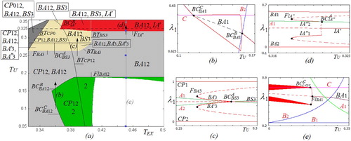
Indeed, in our interpretation, we focused on two options: a soft separation ($T_{EX}=0.35$) and a hard separation ($T_{EX}=0.45$). The former did not destroy agglomeration patterns and looking at Figure 7(a) confirms that a deeper integration within the Union may not bring major qualitative effects. Instead, a hard separation led to dispersion of industrial activity. Further integration within the Union will transform significantly this pattern and we analyse this case in more detail. We begin with the case shown in Figure 4(d) (where $L=20$, $T_{EX}=0.45$ and $T_U=0.325$) and decrease $T_U$, we discuss the most relevant points of the ensuing sequence of bifurcations (corresponding to the blue circles indicated in Figure 7(a)). At the beginning, this sequence leads to two new interior attracting fixed points,¹⁸ $I{A}_1^{\mathrm{\prime }\mathrm{\prime }}$ and $I{A}_2^{\mathrm{\prime }\mathrm{\prime }},$ and to the stability loss of the interior equilibrium $I{A}^{\mathrm{\prime }}$, after which map $Z$ has four attractors: the border equilibria $B{A}_1$ and $B{A}_2$ as well as the interior equilibria $I{A}_1^{\mathrm{\prime }\mathrm{\prime }}$ and $I{A}_2^{\mathrm{\prime }\mathrm{\prime }}$ (Figure 8(a), where $T_U=0.32$). After, the attracting ($I{A}_1^{\mathrm{\prime }\mathrm{\prime }}$ and $I{A}_2^{\mathrm{\prime }\mathrm{\prime }}$) and the saddle interior equilibria (which are visible but not labelled in Figures 4(d) and 8(a)) merge in pairs and disappear,¹⁹ leaving only two stable equilibria, $B{A}_1$ and $B{A}_2$ (Figure 8(b), where $T_U=0.25$). By further decreasing $T_U$ the fixed points $B{A}_1$ and $B{A}_2$ undergo a flip bifurcation, so that attractors of $Z$ are two two-cycles on the borders $I_{b1}$ and $I_{b2}$ (Figure 8(c), where $T_U=0.186$). These two-cycles then collide with the border $C$, leading to chaos, namely, to the two-cyclic chaotic attractors on the borders $I_{b1}$ and $I_{b2}$. At the same time, the fixed points $C{P}_1$ and $C{P}_2$ become attracting. In Figure 8(d), drawn for $T_U=0.05$, the basins of $C{P}_1$ and $C{P}_2$ are shown in green (dark grey) and dark blue (light grey), respectively.²⁰

Figure 8. Coexisting attractors of map $Z$ and their basins for $T_{EX}=0.45,$ $L=20$ and (a) $T_U=0.32$, (b) $T_U=0.25$, (c) $T_U=0.186$ and (d) $T_U=0.05$ (see the blue circles in Figure 7(a)). The other parameters are fixed as in (17).

Recall (see Figure 4(d)) that a hard separation may lead to two different outcomes. The first possibility is the equilibrium $I{A}^{\mathrm{\prime }}$, industry is located in all regions and the trade network structure is of the $NS3$ type, that is, bilateral between the regions in the Union, while $R_3$ is autarkic. Alternatively, a hard separation may lead to $B{A}_1$ or $B{A}_2$, where industry is located in $R_3$ and in only one of the regions in the Union (while the other is left peripheral and without industry) and trade involves only exports from the two industrialized regions towards the peripheral region within the Union ($NS4$).

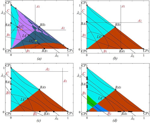
All panels in Figure 8 start from a hard separation scenario (i.e., $T_{EX}=0.45$); the panels depict an increasing internal integration ($T_U$ reduces from $0.32$ to $0.05$). Notice that in all panels $I{A}^{\mathrm{\prime }}$ has lost stability; thus, the Union’s deeper integration after a hard separation destabilizes the symmetric location of industry across the Union. Looking at Figure 8(a), two additional results emerge. First, two new interior fixed points off the diagonal appear that introduce an asymmetry between the regions in the Union. They are located in area $NS2$, where only one-way trade occurs within the Union, from the more to the less industrialized region; $R_3$ remains autarkic (as in $I{A}^{\mathrm{\prime }}$). Second, the basins of attraction of these two equilibria show an intermingled structure, implying that it is difficult to predict which of the two regions will attract the larger industry share (this holds in particular for initial conditions close to $B{S}_3$, in which the regions in the Union are almost symmetric). These additional new equilibria disappear for an even deeper integration within the Union.

The two other possible equilibria, $B{A}_1$ and $B{A}_2$, persist – first as fixed points coexisting with the new interior fixed points (Figure 8(a)); then as the only fixed points (Figure 8(b)); after they lose stability and are substituted first by cycles of period 2 (Figure 8(c)) and finally by two-piece chaotic attractors that coexist with the stable $C{P}_1$ and $C{P}_2$ equilibria. Figure 7(e), that focuses on $B{A}_1$ ($B{A}_2$ is symmetric), allows one to analyse these equilibria in more detail (recall that for the hard separation scenario depicted in Figure 4(d), $T_{EX}=0.45$ was assumed).

First, note that deeper integration within the Union will attract firms from region $R_3$ to the industrialized region within the Union, its share in industry increases. Second, and most interestingly, the trade pattern changes as well, as can easily be seen from Figure 7(e) (note that the $A_1$ line is not relevant, since the equilibrium $B{A}_1$ does not involve industry in $R_2$): initially, for $T_U=0.325$ (Figure 4(d)) and $T_U=0.32$ (Figure 8(a)), ${\lambda }_1$ was on the right of the $B_1$ line and below the $B_2$ line, corresponding to $NS4$ (involving one-way trade from the two industrialized regions to the peripheral region within the Union). Reducing $T_U$, the trade pattern changes, once ${\lambda }_1$ has crossed the $B_2$ line and enters the area $NS2$ ($T_U=0.25$, Figure 8(b); see also Figure 2(d)): the one-way trade from the industrialized region in the Union to the peripheral one continues, but $R_3$ is autarkic and does not export anymore to the peripheral region. $B{A}_1$ and $B{A}_2$ lose stability and give rise to cyclical behaviour. In Figure 8(c), the two-cycles do not collide yet with the border $C$ and the trade pattern does not change: these cycles still involve only trade from $R_1$ to $R_2$ (in $B{A}_1$) or from $R_2$ to $R_1$ (in $B{A}_2$). As $T_U$ is further reduced, the period 2 cycles hit the border $C$. Some of the points of the ensuing two-piece chaotic attractor lie above the $C$ border, thus in $NS8$. In these points, the share of firms located in $R_3$ is sufficiently small that firms located in $R_1$ find it profitable to export towards $R_3$ as well.

Thus, if one of the regions in the Union is peripheral without industry, it will always import from the other region in the Union. $R_3$ does not export to the industrialized region in the Union. With deeper integration in the Union, $R_3$ will stop exporting to the peripheral region in the Union; it is autarkic for some values of $T_U$, before it starts importing from the industrialized region in the Union. As shown in Figure 8(d), other possible outcomes are $C{P}_1$ and $C{P}_2$, whose basins of attraction are intermingled, making the prediction of the long-run position more difficult the closer the initial condition is to $C{P}_0$. In $C{P}_1$ and $C{P}_2$, the core, which is in the Union, exports to the other two regions.

In summary, deeper integration of the Union after a hard separation involves a loss of stability for the interior equilibrium $I{A}^{\mathrm{\prime }}$. One interesting result is that the reduction in $T_U$ may destroy reciprocal trade within the Union. It also reduces the likelihood of $R_3$ exporting towards the Union and increases that of non-trading or importing. Other interesting phenomena can emerge like cyclical or even chaotic behaviour, intermingled basins of attraction and unpredictability of long-run outcomes concerning the location of industry and the patterns of trade.

CONCLUSIONS

As many empirical studies suggest, Brexit will deeply affect Europe’s economic landscape, in particular firm location and trade patterns will change substantially with marked differences between the regions. Empirical studies treat these two dimensions as rather unrelated, whereas an NEG perspective suggests that they are intimately related. In this paper, taking inspiration from the Brexit issue, we fill a gap in the literature exploring the consequences of splitting an integration area or “Union”. To this purpose, we developed a three-region FE model with linear demand functions that allows an explicit analysis of changes in trade patterns. Given the notorious analytic complexity of multiregional NEG models, we primarily present simulation results.

In order to structure our analysis, we differentiated the two situations before separation that are quintessential from an NEG perspective. The relation between market size and trade costs was initially such that the Union was a well-integrated economic area. In that case, NEG models predict (partial or full) agglomeration of economic activity; indeed, we found four agglomeration patterns that are different from an economic point of view. We introduced the splitting of an integration area as an increase in trade cost towards the exiting region (whereas the trade costs remain fixed within the Union); and we differentiated between a soft and a hard separation (in analogy with the two Brexit options), the latter involving a more pronounced increase in trade costs. Our analysis suggests a reduction of trade between the Union and the leaving region, and an intensification of trade within the Union; in many cases firms relocate from the exiting region towards the Union in order to gain market access – in these cases, firm relocation replaces an export link. Remarkably, even a region that was peripheral before separation with no industry may gain industry after separation (being now a region offering access to the Union’s market as well as offering low local competition). In some cases, we also found firm relocation from within the Union to the exiting region, seeking shelter from the intensive competition within the Union.

Alternatively, the ante separation relation between market size and trade costs was initially such that the Union was less integrated. An NEG perspective suggests dispersion of economic activity and a full trade network, which we represented by our second parameter set. In that case, disintegration does only gradually affect industry location; all regions maintain industry, though asymmetries between the leaving and the remaining regions will develop (the latter maintain their symmetry). With a soft separation, the leaving region actually gains industry (firms seeking shelter from competition), the full trade network continues to exist. A harder separation involving a more pronounced increase in trade cost will destabilize the equilibrium and cyclical or chaotic patterns of industry location emerge. Most interesting, these changes in the number of firms and thus in the degree of local competition will also affect trade patterns: bilateral trade within the Union will persist; (unilateral) trade between the regions in the Union and the exiting region will only happen with low competition in the destination region (i.e., a low number of firms). With very high trade costs, firms in the exiting region will stop to export.

Finally, we studied the effects of a deeper integration within the Union after one of the regions has left the Union, starting from a scenario before separation where a well-integrated economic area displays agglomeration features. We find that deeper integration within the Union may actually reverse the effect of a hard separation on industry location, the peripheral region may again (partly or fully) lose their industry. Trade patterns, however, will continue to show a rather isolated position of the exiting region.

Economic disintegration will change trade costs implying corresponding changes in trade patterns and industry location. As a consequence, economic agents’ welfare will change accordingly, since the range of available commodities will vary together with their price (due to transport costs and more/less intense local competition), for the mobile factor – entrepreneurs – profit income changes as well. The overall effect is difficult to ascertain, and we leave this to further research. However, in many instances we found for the leaving region a reduction in trade, in the number of firms and thus in local competition. These factors – taken in isolation – reduce welfare in the leaving region, an aspect that deserves more attention in any discussions on situations of trade disintegration analogous to the Brexit case.

ACKNOWLEDGEMENTS

The authors thank the participants at The Economy as a Spatial Complex System (ESCoS-CICSE 2018) conference, Naples, Italy, and at workshops in Ancona (Italy), Nottingham (UK) and Urbino (Italy). I. Sushko thanks the University of Urbino for the hospitality experienced during her stay there as a visiting professor. I. Kubin thanks the University of Urbino and the University of Nottingham for their hospitality during her research stay.

DISCLOSURE STATEMENT

No potential conflict of interest was reported by the authors.

Additional information

Funding

This work was supported by the WU Vienna University of Economics and Business and by the Austrian National Bank.

Notes

1 NUTS = Nomenclature of Territorial Units for Statistics.

2 Our contribution is in the spirit of Oyama (2009), where, in the context of a two-region FE model with isoelastic demand functions, asymmetric trade costs are introduced. Thus, trading between regions is more or less costly depending on the direction of trade.

3 That remoteness does not necessarily represent a disadvantage has been stressed also by Behrens, Gaigne, Ottaviano, and Thisse (2006) in a two-country/four-region FE model. Their framework of analysis differs from that in this paper in some very relevant respects: (1) firms cannot move across all regions (their mobility being allowed only within a country); and (2) trade costs are sufficiently low to allow for bilateral trade between any pair of regions, so that only a unique trade network structure is possible, that is, the full trade network.

4 The assumption $\text{β}>\delta$ also ensures that the utility function (1) is strictly concave, which is needed for interior solutions to the utility maximization problem (see also Behrens, 2004, p. 89).

5 These network structures are known in the language of SNA as triads.

6 More in detail: crossing $A_1$, if ${\lambda }_1\ge (<)\tilde{\lambda }$, trade from $R_2$ to $R_1$ it is not allowed (it is allowed); crossing $A_2$, if ${\lambda }_2\ge (<)\tilde{\lambda }$, trade from $R_1$ to $R_2$ it is not allowed (it is allowed); crossing $B_1$, if ${\lambda }_1\ge (<)\overline{\lambda }-k{\lambda }_2$, trade from $R_3$ to $R_1$ it is not allowed (it is allowed); crossing $B_2$, if ${\lambda }_2\ge (<)\overline{\lambda }-k{\lambda }_1$, trade from $R_3$ to $R_2$ it is not allowed (it is allowed); and crossing $C$, if ${\lambda }_1\le (>)1-\overline{\lambda }-{\lambda }_2$, trade from $R_1$ to $R_3$ and from $R_2$ to $R_3$ it is not allowed (it is allowed).

7 As would be expected, the transition from more to less connected network structures mostly involves the loss of links connecting the exiting region ($R_3$) with one or both the regions in the Union ($R_1$ and $R_2$).

8 Property 2 implies that the phase portrait of map $Z$ is symmetric with respect to $D$, that is, any invariant set $\mathcal{A}$ is either itself symmetric with respect to $D$ or there exists one more invariant set ${\mathcal{A}}^{\mathrm{\prime }}$ symmetric to $\mathcal{A}$.

9 Figures 3–8 are in colour in the online version and are in greyscales in the printed version.

10 An attractor according to the topological definition is a closed invariant set with a dense orbit, which has a neighbourhood, each point of which is attracted to the attractor. An attractor in the Milnor sense (Milnor, 1985) does not require the existence of such a neighbourhood, but only a set of points of positive measure, attracted to the attractor.

11 For short, we say that an invariant set is M attractor if it is attracting in the Milnor sense, but not in a sense of the topological definition.

12 For example, the boundaries denoted by $BT$ and $F$ correspond to the so-called border-transcritical and fold bifurcations, respectively, which involve a change in the stability of the fixed points. The type of fixed point is indicated in the subscript.

13 Given the highly abstract nature of NEG models, it is always difficult to put numbers to the parameters and we do not claim to have calibrated our model. However, Eurostat (2019b) reports that the percentage with a tertiary education of total employment is about 34% in the EU (ranging from almost 50% to a bit more than 20%). Thus, our ratios 1/3 (33%) and 1/4 (25%) appear to be in a reasonable range.

14 This bifurcation sequence can also be understood by looking at Figure 3(a,b) in correspondence of $L=20$ and by increasing $T_{EX}$ starting from 0.325. We see that $C{P}_0$ becomes unstable when the boundary $B{T}_{CP0}$ is crossed, undergoing a border-transcritical bifurcation. $I{A}^{\mathrm{\prime }}$ becomes stable when $T_{EX}$ collides with $B$ (not marked in the Figure), generating a border collision bifurcation (BCB) entering the region $I{A}^{\mathrm{\prime }}$ shown in red. Notice that at the same bifurcation point, a couple of new interior saddle fixed points are born. Finally, the fixed point $B{S}_3$ loses its stability due to a border-transcritical bifurcation when the boundary $B{T}_{BS3}$ is crossed.

15 Border fixed points have already lost their stability via a so-called flip bifurcation, so that on the borders of the triangle $S$ there are saddle cycles (i.e., cycles stable only along one direction) of period 2. In Figure 5(a), these unstable period 2 cycles are represented by dots (grey and orange or blue, respectively) around the corresponding border symmetric fixed point ($B{S}_1$, $B{S}_2$ and $B{S}_3$); in Figure 5(b), when $T_{EX}=0.37$, the two-period cycles around $B{A}_1$ and $B{A}_2$ are replaced by two-piece 1D chaotic attractors on $I_{b1}$ and $I_{b2}$; and in Figure 5(c), when $T_{EX}=0.4$, by a one-piece 1D chaotic attractors on $I_{b1}$ and $I_{b2}$.

16 Specifically, a flip BCB takes place.

17 When $T_{EX}$ is increased even further, the attractor on the diagonal disappears (more precisely, it is transformed into a chaotic repellor) due to a contact with the border $I_{b3}$ (when the parameter point enters the pink region $M$ in Figure 3(a)) after which almost all the initial points of $S$ are attracted to an M attractor belonging to $I_{b3}$ (a 1D chaotic attractor whose points are characterized by no industry in $R3$). This attractor eventually disappears due to a contact with the fixed points $C{P}_1$ and $C{P}_2$, so that they become M attracting. All industry is located in one region of the Union, $R_1$or $R_2$.

18 More specifically, considering the range $0.316<T_U<0.325$ represented in Figure 7(d), a fold BCB gives rise to two couples of interior fixed points (see the label $B{C}_{I{A}^{\mathrm{\prime }\mathrm{\prime }}}^A$) leading to two new interior attracting fixed points, $I{A}_1^{\mathrm{\prime }\mathrm{\prime }}$ and $I{A}_2^{\mathrm{\prime }\mathrm{\prime }},$ and two saddles; these saddles quite soon merge with the fixed point $I{A}^{\mathrm{\prime }}$ and this fixed point loses stability, that is, a reverse pitchfork bifurcation occurs. A maximum of four stable fixed points exists in this range.

19 This occurs via a reverse fold bifurcation (when the curve $F_{I{A}^{\mathrm{\prime }\mathrm{\prime }}}$ is crossed, see also the label $F_{I{A}^{\mathrm{\prime }\mathrm{\prime }}}$ in Figure 7(d)).

20 More specifically, they become M attracting (see note 7 above). This is because the flat branches of the functions defining map $Z$ ‘enter’ the triangle $S.$ Evolution of the attractors on the borders $I_{b1}$ and $I_{b2}$ can be clarified by means of the 1D bifurcation diagram ${\lambda }_1$ versus $T_U$ shown in Figure 7(e) (recall that due to the symmetry of the map the same dynamics is observed on the border $I_{b2}$). In this diagram one can see that a contact of the two-cycle with the border $C$ indeed leads to the two-cyclic chaotic attractor.

REFERENCES

- Ago, T., Isono, I., & Tabuchi, T. (2003). Locational disadvantage and losses from trade, three regions in economic geography. Discussion Paper CIRJE-F-224.
- Ago, T., Isono, I., & Tabuchi, T. (2006). Locational disadvantage of the hub. The Annals of Regional Science, 40(4), 819–848. doi: 10.1007/s00168-005-0030-x
- Baldwin, R., Forslid, R., Martin, P., Ottaviano, G., & Robert-Nicoud, F. (2003). Economic geography and public policy. Princeton, NJ: Princeton University Press.
- Barbero, J., & Zofío, J. L. (2016). The multiregional core–periphery model: The role of the spatial topology. Networks and Spatial Economics, 16(2), 469–496. doi: 10.1007/s11067-015-9285-7
- Behrens, K. (2004). Agglomeration without trade: How non-traded goods shape the space-economy. Journal of Urban Economics, 55(1), 68–92. doi: 10.1016/j.jue.2003.06.003
- Behrens, K. (2005). How endogenous asymmetries in interregional market access trigger regional divergence. Regional Science and Urban Economics, 35(5), 471–492. doi: 10.1016/j.regsciurbeco.2004.06.002
- Behrens, K. (2011). International integration and regional inequalities: How important is national infrastructure? The Manchester School, 79(5), 952–971. doi: 10.1111/j.1467-9957.2009.02151.x
- Behrens, K., Gaigne, C., Ottaviano, G. I., & Thisse, J. F. (2006). Is remoteness a locational disadvantage? Journal of Economic Geography, 6(3), 347–368. doi: 10.1093/jeg/lbi024
- Castro, S. B. S. D., Correia-da-Silva, J., & Mossay, P. (2012). The core–periphery model with three regions and more. Papers in Regional Science, 91(2), 401–418.
- Commendatore, P., Filoso, V., Kubin, I., & Grafeneder-Weissteiner, T. (2015). Towards a multiregional NEG framework: Comparing alternative modelling strategies. In P. Commendatore, S. S. Kayam, & I. Kubin (Eds.), Complexity and geographical Economics: Topics and Tools (pp. 13–50). Heidelberg: Springer.
- Commendatore, P., Kubin, I., & Sushko, I. (2018a). Dynamics of a developing economy with a remote region: Agglomeration, trade integration and trade patterns. Communications in Nonlinear Science and Numerical Simulation, 58, 303–327. doi: 10.1016/j.cnsns.2017.04.006
- Commendatore, P., Kubin, I., & Sushko, I. (2018b). Emerging trade patterns in a 3-region linear NEG model: Three examples. In P. Commendatore, I. Kubin, S. Bougheas, A. Kirman, M. Kopel, & G. I. Bischi (Eds.), The economy as a complex spatial system: Macro, meso and micro perspectives (pp. 38–80). Cham: Springer.
- Commendatore, P., Kubin, I., & Sushko, I. (2018c). The impact of Brexit on trade patterns and industry location: an NEG analysis. Department of Economics Working Paper Series, 267. WU Vienna University of Economics and Business, Vienna.
- Eurostat. (2019a). Regional GDP per capita ranged from 31% to 626% of the EU average in 2017. Eurostat Newsrelease, 34.
- Eurostat. (2019b). Retrieved from https://ec.europa.eu/eurostat/data/database?node_code=lfsi_educ_a
- Gaspar, J. M. (2018). A prospective review on new economic geography. The Annals of Regional Science, 61, 237–272. doi: 10.1007/s00168-018-0866-5
- Gaspar, J. M., Castro, S. B. S. D., & Correia-da-Silva, J. (2019). The footloose entrepreneur model with a finite number of equidistant regions. International Journal of Economic Theory, online first: 1–27. doi: 10.1111/ijet.12215
- Ikeda, K., Akamatsu, T., & Kono, T. (2012). Spatial period-doubling agglomeration of a core–periphery model with a system of cities. Journal of Economic Dynamics and Control, 36(5), 754–778. doi: 10.1016/j.jedc.2011.08.014
- Ikeda, K., Murota, K., & Takayama, Y. (2017). Stable economic agglomeration patterns in two dimensions: Beyond the scope of central place theory. Journal of Regional Science, 57(1), 132–172. doi: 10.1111/jors.12290
- Ikeda, K., Onda, M., & Takayama, Y. (2018). Spatial period doubling, invariant pattern, and break point in economic agglomeration in two dimensions. Journal of Economic Dynamics and Control, 92, 129–152. doi: 10.1016/j.jedc.2018.05.002
- Krugman, P. R. (1980). Scale economies, product differentiation, and the pattern of trade. American Economic Review, 70(5), 950–959.
- Krugman, P. R. (1991). Increasing returns and economic geography. Journal of Political Economy, 99(3), 483–499. doi: 10.1086/261763
- Macron, E. (2017). Initiative for Europe. Speech at La Sorbonne, Sept. 26, 2017. English transcript. Retrieved from https://www.diplomatie.gouv.fr/IMG/pdf/english_version_transcript_-_initiative_for_europe_-_speech_by_the_president_of_the_french_republic_cle8de628.pdf
- Milnor, J. (1985). On the concept of attractor. Communications in Mathematical Physics, 99, 177–195. doi: 10.1007/BF01212280
- Ottaviano, G. I., Tabuchi, T., & Thisse, J. F. (2002). Agglomeration and trade revisited. International Economic Review, 43(2), 409–435. doi: 10.1111/1468-2354.t01-1-00021
- Oyama, D. (2009). History versus expectations in economic geography reconsidered. Journal of Economic Dynamics and Control, 33(2), 394–408. doi: 10.1016/j.jedc.2008.06.007
- Tabuchi, T., Thisse, J. F., & Zeng, D. Z. (2005). On the number and size of cities. Journal of Economic Geography, 5(4), 423–448. doi: 10.1093/jnlecg/lbh060