Integrating macroeconomics and economic geography: the neoclassical growth model in spatial general equilibrium

ABSTRACT

The neoclassical growth model and the Roback model of spatial general equilibrium (SGE) are integrated to study the joint determination of macroeconomic phenomena (gross domestic product (GDP) and the rate of interest) and spatial economic phenomena (the spatial distribution of gross regional product (GRP), employment and capital). If internal capital mobility is perfect and regional savings rates are homogeneous, GDP depends on SGE, but SGE does not depend on GDP. If saving rates are spatially heterogeneous, GDP and the rate of interest depend on SGE, but SGE does not depend on the rate of interest and GDP. If in addition capital is imperfectly mobile, macroeconomic outcomes such as GDP, the rate of interest and SGE are jointly determined. In general, therefore, the dichotomy between macroeconomics and economic geography breaks down.

KEYWORDS:

• spatial general equilibrium
• neoclassical growth model
• Roback model
• integrating macroeconomics and economic geography

JEL:

• O18
• O41
• R13

1. INTRODUCTION

Macroeconomic theory has by default treated space as a seamless whole. By implication it makes no macroeconomic difference where productivity or other macroeconomic shocks occur. By contrast, it has been difficult for economic geographers to avoid macroeconomics because the gross domestic product (GDP) is the sum of gross regional products (GRPs). However, they have stopped short of synthesising economic geography with canonical macroeconomic issues such as the determination of interest rates. Nor have they studied the dependence of the spatial economy on these macroeconomic phenomena. The two-way integration of macroeconomics and economic geography remains a theoretical lacuna, which is our focus here.

Spatial general equilibrium (SGE) theory (Krugman, 1991; Roback, 1982) has been largely concerned with the spatial distribution of economic activity in general and the spatial distribution of people in particular. This tradition dates back to Hicks (1932) who drew attention to internal labour mobility for the spatial distribution of wages and economic activity. Roback and Krugman gave formal expression to this tradition; the former by assuming that the ‘quality of life’ varies across space, trade is costless and competition is perfect, and the latter by assuming trade is costly, competition is imperfect and the quality of life is homogeneous. Both Roback and Krugman did not consider the role of capital and related macroeconomic phenomena such as national savings and investment, the rate of interest and economic growth.

Subsequently, Krugman’s ‘New Economic Geography’ (NEG) model was developed and modified for different purposes. A disadvantage of NEG over Roback is that NEG is not amenable to analytical solution; it has to be simulated numerically. Attempts to simplify NEG to make it amenable to analytical solution undermined its spirit by abstracting from internal labour mobility (Beenstock, 2020). The same criticism applies to the extensive literature on the implications of NEG for endogenous economic growth reviewed below. Whereas the mobility of capital and goods and the immobility of labour are standard assumptions in open-economy macroeconomics, the mobility of labour is a feature sine qua non of SGE theory. In any case there is more to macroeconomics than economic growth.

In summary, there is currently no NEG-type model that combines the mobility of labour, capital and goods. There is certainly no NEG-type model, which integrates saving, investment, the rate of interest and economic growth. Economic geography and macroeconomics remain apart.

Whereas NEG has attracted much attention in the literature, Beenstock (2020) extended the Roback model to include capital mobility, which intensifies the effect of local productivity shocks on GDP. These results demonstrated theoretically and empirically (Beenstock, 2021) that the spatial economy matters for aggregate supply. However, these efforts assumed that the spatial distribution of economic activity is independent of macroeconomic developments.

This paper attempts to integrate macroeconomics and SGE theory in both directions. A full integration between macroeconomics and SGE requires a self-contained macroeconomic model as well as an SGE model in which goods, labour and capital are internally mobile. The present paper does this for the first time. Specifically, the neoclassical single sector growth model is ‘spatialised’ so that macroeconomic and spatial equilibrium are jointly determined. The model refers to a closed economy in which labour and capital are spatially mobile, and frictionless trade takes place in the single good. As in Beenstock (2020) spatial heterogeneity in the quality of life implies that labour mobility is imperfect. At first capital is assumed to be perfectly mobile. Subsequently, the latter assumption is relaxed on the grounds that the productivity of capital may be location specific; just as wages are not equated across space, nor are returns to capital. Also, savings ratios are assumed to be spatially heterogeneous. The capital market is open internally so savers may invest in locations in which they do not reside.

These assumptions provide the theoretical underpinnings for the mutual integration of macroeconomics, as represented by neoclassical growth theory, and SGE as represented by the extended Roback model. The joint determination of macroeconomic phenomena such the rate of interest, saving, investment and economic growth, are mutually integrated with spatial phenomena such GRP and the spatial distribution of labour, capital, wages and profits.

Regional economists have applied the neoclassical growth model in regional contexts with the intention of introducing dynamics into models of spatial equilibrium (Harris, 2011). However, this literature treats regions as independent economies between which labour and capital are immobile. The present paper complements this literature by relaxing the restrictions that labour and capital are internally immobile.

Several new theoretical results are established. First, if savings rates are spatially homogeneous and capital is perfectly mobile, the rate of interest is independent of SGE, but GDP is not. Second, if capital is perfectly mobile, but regional savings rates are heterogeneous, both GDP and the rate of interest depend on SGE, but there is still no feedback from macroeconomics to SGE. Third, if additionally, capital is imperfectly mobile, GDP and the rate of interest depend upon SGE, and SGE depends upon the rate of interest. Macroeconomic theory and SGE theory are mutually inseparable. Fourth, the way in which they are mutually inseparable depends on the spatial distribution of total factor productivity (TFP) and savings rates.

Although these results may be model specific, our purpose here is to establish preliminary conditions under which the traditional dichotomy between macroeconomics, represented by the neoclassical growth model, and economic geography, represented by the Roback model, is breached. Section 2 sets out the basic theory when there are two spatial units. Subsequently, we discuss generalisations. The basic theory concerns the determination of the rate of interest when aggregate supply depends upon SGE, but not the other way around. In section 3, conditions are established under which SGE depend on the rate of interest. Section 4 studies the macroeconomy and the spatial economy under joint macroeconomic and SGE.

The present paper has most in common with Rappaport (2004) who investigated the relation between a small open region characterised by Roback, and a large region characterised by the neoclassical growth model. Capital, goods and labour are mobile between the large and small region. What happens in the small region depends on the large region, but not vice versa. By contrast, the present paper allows both regions to be mutually dependent; hence the rate of interest determined by the neoclassical growth model depends on developments in both regions.

2. LITERATURE REVIEW

International economic theory studies the dependence between countries induced by cross-border trade and capital movements in the absence of international migration, but when countries have different exchange rates. SGE theory studies the dependence between regions induced by internal migration, trade and capital mobility when regions share common exchange rates. The canonical NEG model is concerned with trade and internal migration, in the absence of capital. There are two sectors, ‘manufactures’ in which competition is imperfect, and ‘agriculture’ in which competition is perfect. Agriculture and manufactures are produced in different regions and are produced with skilled and unskilled labour. Skilled labour is mobile between regions but unskilled labour is immobile. Interregional trade in agriculture is costless, but trade in manufactures is costly.

Numerous variants of the NEG model have been proposed. However, there is no variant, which combines internal migration, trade and capital mobility. Whereas all variants refer to trade, variants which combine capital mobility (Baldwin & Martin, 2004; Baldwin et al., 2003, ch. 2; Davis & Hashimoto, 2014, 2015; Yamamoto, 2003) assume that labour is internally immobile, and variants which combine internal migration (Baldwin & Forslid, 2000; Bond-Smith, 2021; Bond-Smith et al., 2018; Kichko, 2018) ignore capital and its mobility. Yet further variants have neither labour mobility nor capital mobility (Davis, 2009). Rappaport (2004) is the only study to combine trade, internal migration and capital mobility in a small region, when the spatial equilibrium in the large region is exogenous.

In their final chapter, Brakman et al. (2009) discuss the implications of NEG for economic growth in reference to Baldwin and Forslid (2000) and Baldwin and Martin (2004). The latter is based on the ‘footloose capital’ model (Baldwin et al., 2003, ch. 3; Forslid & Ottaviano, 2003) in which skilled labour is assumed to be immobile between regions, but capitalists are perfectly mobile. Since the immobility of skilled labour is a major departure from the NEG model, the implications of these studies for economic growth are arguably too removed from the original (Beenstock, 2020).

Davis and Hashimoto (2015) refer to ‘footloose capital’ as ‘footloose production’ where firms relocate costlessly to regions where production costs are lowest. ‘Footloose firms’ morph into ‘footloose skilled labour’ where skilled labour is defined as entrepreneurs who engage in the development of new products, which are produced by unskilled labour (Bond-Smith et al., 2018; Bond-Smith & McCann, 2020). Unsurprisingly, these semantic roles attributed to skilled labour as well as the assumptions regarding costless relocation generate analytical solutions, but they are arguably significant departures from the NEG model.

Matters are different for Baldwin and Forslid (2000) who extend the canonical NEG model by assuming that there is a fixed cost to establishing new varieties of manufactures. They also assume that this fixed cost varies inversely with the number of local varieties plus a spillover factor multiplied by the number of varieties in other regions. Hence, as the number of varieties grows, it becomes cheaper to establish new varieties. If the local region is initially more populated, it has a growth advantage, which induces inward migration and agglomeration.

This mechanism of endogenous growth is borrowed from first-generation non-spatial endogenous growth theory. Bond-Smith (2021) has noted that this practice ignores the fact that Marshallian and Jacobs scale effects are peculiarly local; unlike blueprints they are not spatially transferable. First generation endogenous growth theory assumed fixed populations because population growth induced ever increasing economic growth. Bond-Smith notes that these scale effects induce unintended economic growth in agglomerating regions. By contrast, semi-endogenous non-spatial growth theory (Jones, 1995) is scale-neutral because it assumes that innovation becomes increasingly costly, whereas Young (1998) and Peretto (1998) proposed a fully endogenous second-generation growth model without scale effects. Bond-Smith (2021) has suggested combining the latter in SGE theory of endogenous growth which is quintessentially spatial.

In summary, there is no version of NEG that combines internal mobility of labour and capital and in which endogenous growth is inherently spatial. Also, economic growth is driven by the accumulation of knowledge because there is no capital in NEG. These extensions of NEG do not engage with mainstream macroeconomics. They may shed light on spatial aspects of endogenous growth, but they can hardly be considered as contributions to macroeconomic theory. Perhaps this explains why this literature has been overlooked by macroeconomists.

3. SINGLE-SECTOR TWO-REGION ‘ROBACK’ NEOCLASSICAL GROWTH

Representing macroeconomics by the neoclassical single sector growth model, and SGE by the two-location Roback model makes for a minimalist theory in which to study the mutual dependence between macroeconomics and economic geography.

3.1. Indirect utility and residency irrelevance

Individuals are assumed to behave as in the Ramsey (1928) model; they save in order to maximise the present value of consumption discounted by the rate of time preference ρ. In the present context, income from capital originates either from where they work and live, or it originates from elsewhere. Since they have free access to capital markets they do not have to live in a location to own capital there. However, to access labour markets they must live in the location where they work because there is no commuting. Residency irrelevance applies to income from capital but not from labour.

Their indirect utility function for choosing to live in location j is: (1a) $U_{\mathrm{ij}}=u[(1-s_j)(w_j+c_i)]+q_{\mathrm{ij}}$(1a) where i labels individuals, w_j denotes the wage in location j, s_j denotes the steady-state savings rate in location j, and q_ij denotes the unobserved quality of life (in the sense of Roback) experienced by individual i from living in location j. Income from capital (c) does not depend on j because of residency irrelevance. It comprises income from capital in the location of residence as well as from other locations. Its determination is discussed in detail below. Equation (1a) assumes that individuals assimilate to the steady-state savings rate in their chosen location.

Let j = 1, 2 because there are two locations, and assume for the moment that s₁ = s₂ = s. Individual i chooses to reside in location 1 during period t if U_i1t > U_i2t. If u( ) is separable, for example, $u_t=\theta \ln [(w_{\mathrm{jt}}(1-s_j)]+\varphi \ln [c_t(1-s_j)]$, individual i resides in location 1 during period t when: (1b) $U_{i1t}-U_{\mathrm{ist}}=\mathrm{\theta ln}{\displaystyle \frac{w_{1t}(1-s_1)}{w_{2t}(1-s_2)}+q_{i1t}-q_{i2t}>0}$(1b) Notice that capital income does not feature in equation (1b) due to ‘residency irrelevance’. The expected value of q_i1 – q_i2 is zero with standard deviation σ if it is normally distributed, and with standard deviation $\mathrm{\pi \sigma }/\sqrt{3}$ if it is logistically distributed. The latter exceeds σ due to its fatter tails. Equation (1b) implies that relocation costs are zero. It also implies that infra-marginal individuals (where the sign of U₁ – U₂ may fluctuate) relocate frequently. However, if q_ij is time invariant, relocation depends only on changes in relative wages.

3.2. Spatial general equilibrium (SGE)

In what follows Y, A and L denote homogenous output, total factor productivity (TFP) and employment, respectively. Gross regional products (GRP) are produced by Cobb–Douglas technologies, and GDP (Y) is the sum of GRPs: (2) $Y_t=A_1({\kappa }_t{K}_t{)}^{\alpha }({\pi }_t{L}_t{A}_t{)}^{1-\alpha }+A_2[(1-{\kappa }_t)K_t{]}^{\alpha }[(1-{\pi }_t)L_t{A}_t{]}^{1-\alpha }$(2) where κ denotes the share of capital located in region 1 and π denotes its population share. For simplicity, we assume that TFP in regions 1 and 2 grows at the same exogenous rate (a), hence A_t = A₀exp(a_t), but the levels of TFP differ because A₁ and A₂ differ. Note that despite appearances, technical progress is not necessarily labour augmenting since $a=[\mathrm{\alpha b}+(1-\alpha )\lambda ]/(1-\alpha )$ where b and λ denote the rates of capital and labour augmenting technical progress (Barro & Sala-i-Martin, 2004, p. 79).

Equation (2) may be expressed in terms of national output per head and the capital–labour ratio in terms of efficiency units: (2a) ${\tilde{y}}_t={\displaystyle \frac{Y_t}{A_0\exp (\mathrm{at})L_t}={\mathrm{\Omega }}_t{\tilde{k}}_t^{\alpha }}$(2a) (2b) ${\mathrm{\Omega }}_t=A_{1t}{\omega }_{1t}+A_{2t}{\omega }_{2t}$(2b) (2c) ${\omega }_{1t}={\kappa }_t^{\alpha }{\pi }_t^{1-\alpha }{\omega }_{2t}=(1-{\kappa }_t{)}^{\alpha }(1-{\pi }_t{)}^{1-\alpha }$(2c)

We refer to Ω as the ‘SGE factor’ because it reflects the spatial distribution of capital, labour and TFP. Beenstock (2020) has demonstrated that when capital is perfectly mobile, and q_i1 – q_i2 has an extreme value type 1 distribution (logit), equations (1b) and (2) imply the following solutions for relative wages and savings rates, and the shares of labour and capital in location 1: (3a) $R={\displaystyle \frac{w_1(1-s_1)}{w_2(1-s_2)}={\displaystyle \frac{1-s_1}{1-s_2}{\left({\displaystyle \frac{A_1}{A_2}}\right)}^{\frac{1}{1-\alpha }}}}$(3a) (3b) $\pi ={\displaystyle \frac{1}{1+\exp \left(-{\displaystyle \frac{\theta \sqrt{3}}{\mathrm{\pi \sigma }}\mathrm{lnR}}\right)}}$(3b) (3c) ${\displaystyle \frac{\kappa }{1-\kappa }={\displaystyle \frac{\pi }{1-\pi }R}}$(3c)

Equation (3a) states that the relative wage in region 1 varies directly with its relative TFP for given steady-state savings rates. Equation (3b) states that when people are imperfectly mobile because they have preferences for location specific amenities (quality of life) region 1’s population share varies directly with its relative wage and inversely with its relative steady-state savings rate, and it varies inversely with σ. The latter effect arises because when σ is larger fewer individuals satisfy equation (1b) conditional on the relative wage. It is well known (Maddala, 1983, pp. 22–23; Greene, 2012, p. 726) that θ and σ cannot be identified with binary data, but θ/σ is clearly identified in equation (3b). Notice that due to residency irrelevance, capital income does not feature in equation (3b). Equation (3c) states that when capital is perfectly mobile, the ratio of regional capital shares varies proportionately with the ratio of population shares, the wage ratio net of savings.

If TFP and steady-state savings rates are the same in regions 1 and 2 (A₁ = A₂, s₁ = s₂), wages are equated (R = 1), population and capital shares are the same (π = κ = 0.5) and Ω = A.

Since relocation costs are zero and capital is perfectly mobile, equations (3) apply in every time period; hence, time subscripts are dropped. Equations (3) characterise the SGE for Cobb–Douglas technologies in which π, κ and R depend only on relative TFP (A₁/A₂). Since relative TFP is fixed by assumption, Ω is independent of time. For this reason, it is also independent of capital accumulation.

For Cobb–Douglas technologies in which the elasticity of substitution between labour and capital is one, Ω is independent of population and capital shares because ω₁ + ω₂ = 1. For CES technologies the SGE parameter (Ω) varies directly with region 1’s factor shares when the elasticity of substitution exceeds 1 and inversely when it is less than 1 (Beenstock, 2020). Here, for expositional simplicity, we focus on the Cobb–Douglas case.

The SGE factor (Ω) is entirely endogenous. The spatial distribution of TFP and steady-state savings rates determines the spatial distribution of labour (π) and capital (κ), which determines Ω as in equation (2b).

3.3. Spatial and macroeconomic growth equilibria

Locations 1 and 2 are initially assumed to share a common savings rate (s). In the steady-state, national savings equal investment: (4a) $s{\tilde{y}}_t=(n+\delta +a){\tilde{k}}_t$(4a) where n denotes the rate of national population growth and δ the rate of capital depreciation. Substituting equation (2a) into equation (4) solves for the steady-state solution for the capital–labour ratio in terms of efficiency units: (4b) ${\tilde{k}}^{\ast }={\left({\displaystyle \frac{s\mathrm{\Omega }}{n+\delta +a}}\right)}^{\frac{1}{1-\alpha }}$(4b)

The equilibrium capital–labour ratio varies directly with the savings ratio, and inversely with n + δ + a, as expected in the Solow–Swan neoclassical growth model. However, it also varies directly with Ω, which depends on the regional distributions of capital, labour and TFP.

The same applies to ‘golden rule’ savings rates in which the gross marginal productivity of capital equals n + δ + a. Hence, the steady-state solution in equation (4b) implies that consumers dynamically optimise consumption and the capital stock is a state variable, which grows at the rate of n + a in the steady state. GDP and GRP per capita grow at the rate a in the steady state, and Ω does not change because relative TFP remains constant between locations. In the steady-state the marginal productivity of capital is constant at: (4c) $\alpha \mathrm{\Omega }({\tilde{k}}^{\ast }{)}^{\alpha -1}=\mathrm{MP}{K}^{\ast }$(4c)

Consequently, the rate of interest in the steady-state equals $r^{\ast }=\mathrm{MP}{K}^{\ast }-\delta$, at which national saving equals investment. Substituting equation (4b) into equation (6c) establishes that the rate of interest (r) is independent of the SGE factor (Ω): (4d) $r=\alpha {\displaystyle \frac{n+\delta +a}{s}-\delta }$(4d)

As usual in neoclassical growth models, the rate of interest varies directly with the rates of population growth and technical change, and it varies inversely with the rate of depreciation if $<s$. In summary, levels of GDP and capital depend on the SGE factor (Ω) but growth rates and the rate of interest do not. Also, Ω depends entirely on relative TFP between regions 1 and 2. If relative TFP increases when TFP in region 1 is larger than in region 2, the capital stock increases, which raises GDP both directly and indirectly via equation (2b). The relative wage in region 1 increases via equation (3a), which increases region 1’s population share via equation (3b), and its capital share via equation (3c).

In the Ramsey–Cass neoclassical growth model, in which the rate of saving is optimal, the steady-state saving rate is: (5a) $s=\alpha {\displaystyle \frac{\delta +a+n}{\delta +\rho +\mathrm{\epsilon a}}}$(5a) where the marginal utility of consumption (ϵ) and the rate of time preference (ρ) are assumed to be constant (Barro and Sala-i-Martin, 2004, p. 100). Substituting equation (5a) into equation (4d) implies that the rate of interest is: (5b) $r=\delta +\rho +\mathrm{\epsilon a}$(5b) and the marginal productivity of capital in the steady state is: (5c) $\mathrm{MP}{K}^{\ast }=\rho +\mathrm{\epsilon a}$(5c)

Since the steady-state savings rates are assumed here to be the same, the rate of time preference (ρ) and ϵ are the same in both locations.

3.4. Regional savings rates

Savings rates differ when ϵ and ρ differ between locations. By implication when individuals relocate they assimilate by adopting ϵ and ρ in their new location. When savings rates differ, residency depends on savings rates through equation (1b) because indirect utility varies inversely with savings rates. If savings rates happen to differ between regions, it may be shown that the rate of interest is no longer independent of SGE. In this case, equation (4b) becomes: (6a) $r=\alpha \left({\displaystyle \frac{\mathrm{\Omega }(n+\delta +a)}{s_1{A}_1{\omega }_1+s_2{A}_2{\omega }_2}}\right)-\delta$(6a) where s₁ and s₂ denote savings rates in regions 1 and 2. Note that when the savings rates are the same, equation (6a) reverts to equation (4d). An increase in TFP in region 1 induces an increase in ω₁ and an equivalent decrease in ω₂ (in the Cobb–Douglas case). Note that ω₁ varies inversely and ω₂ directly with the relative savings rate in location 1. Equation (6a) implies that the effects of productivity shocks on the rate of interest are ambiguous. By differentiating equation (6a) with respect to A₁, it may be shown the rate of interest varies inversely with TFP in location 1 when: (6b) $[{\omega }_2(A_1-A_2)(s_1{A}_1-s_2{A}_2)+A_1{A}_2(s_2-s_1)]{\displaystyle \frac{\mathrm{\partial }{\omega }_1}{\mathrm{\partial }{A}_1}<0}$(6b) where $\mathrm{\partial }{\omega }_1/\mathrm{\partial }{A}_1>0$ is positive according to equations (3) and ω₂ is a fraction. Equation (6b) implies, as expected, that if TFP is the same, productivity shocks in location 1 reduce the rate of interest if the savings rate in location 1 is larger than in location 2. The same applies when productivity weighted savings rates are the same. If TFP and the savings rate in location 1 are larger than in location 2, equation (6b) implies that the rate of interest varies directly with TFP in location 1 provided the difference between the savings rates is sufficiently small. More generally, equation (6b) implies that the effect of productivity shocks on the rate of interest is ambiguous.

3.5. Gross domestic and gross national regional products

Let GDRP denote gross ‘domestic’ regional product and GNRP denote gross ‘national’ regional product, defined as in standard national income accounting as GDRP plus net factor income from other locations. Let K₁₂ denote the capital in location 2 owned by residents of location 1. Hence, the GNRPs in locations 1 and 2 are: (7a) $\mathrm{GNR}{P}_1=\mathrm{GDR}{P}_1+K_{12}\mathrm{MPK}$(7a) (7b) $\mathrm{GNR}{P}_2=\mathrm{GDR}{P}_2-K_{12}\mathrm{MPK}$(7b) where, if capital is freely mobile, MPK denotes the common return on capital in both locations. Since the national economy is closed GDP = GNP = GDRP₁ + GDRP₂ = GNRP₁ + GNRP₂.

K denotes the national capital stock, of which κK is located in location 1 and (1 – κ)K is located in location 2. The steady-state share of national capital owned by residents of location 1, denoted by φ, depends on the share of location 1’s savings in national savings: (7c) $\phi ={\displaystyle \frac{s_1{A}_1{\omega }_1}{s_1{A}_1{\omega }_1+s_2{A}_2{\omega }_2}}$(7c) which varies directly with relative savings rates, relative TFP and relative ω. Hence, K₁₂ equals: (7d) $K_{12}=(\phi -\kappa )K$(7d)

Notice that if φ > κ, K₁₂ is positive; residents of location 1 own more capital than is located in location 1 in which event GNRP in location 1 is greater than GDRP. If φ > κ, K₁₂ is negative; residents of location 2 own more capital than is located in location 2, in which event GNRP in location 1 is less than GDRP.

In the previous subsection savings were assumed to depend on GDRP. When savings depend on GNRP the rate of interest depends on the ownership of capital as well as its location. The counterpart to equation (4a) is: (7e) $[s_1{A}_1{\omega }_1+s_2{A}_2{\omega }_2+\mathrm{MPK}(\phi -\kappa )(s_1-s_2)]{\tilde{k}}^{\alpha }=(n+a+\delta )\tilde{k}$(7e) Notice that when φ = κ, equation (7e) reduces to equation (6a) as the solution for the rate of interest; because both locations own their own capital, they are autarkic. Notice also that when φ and κ differ, equation (7e) is non-linear in $\tilde{k}$ because $\mathrm{MPK}=\alpha \mathrm{\Omega }{\tilde{k}}^{\alpha -1}$. Substituting for MPK in equation (7e) generates the following quadratic equation in ${\tilde{k}}^{\alpha -1}$: (7f) $\alpha \mathrm{\Omega }(\phi -\kappa )(s_1-s_2){\tilde{k}}^{2(\alpha -1)}+(s_1{A}_1{\omega }_1+s_2{A}_2{\omega }_2){\tilde{k}}^{\alpha -1}-(n+a+\delta )=0$(7f) The positive root (ρ₊) of equation (7f) is: (7g) ${\tilde{k}}^{\alpha -1}={\displaystyle \frac{-(s_1{A}_1{\omega }_1+s_2{A}_2{\omega }_2)+\sqrt{{(s_1{A}_1{\omega }_1+s_2{A}_2{\omega }_2)}^2+4(n+a+\delta )\alpha \mathrm{\Omega }(\phi -\kappa )(s_1-s_2)}}{2\alpha \mathrm{\Omega }(\phi -\kappa )(s_1-s_2)}}$(7g) Finally, the rate of interest is: (7h) $r=\alpha \mathrm{\Omega }{\rho }_{+}-\delta$(7h) Table 1 compares the solutions for equations (6a) and (7h) under the assumptions A₁ = A₂ = 1, (hence, ω₁ = ω₂ = κ = 0.5 and Ω = 1), δ = 0.1, α = 0.3 and n + a = 0.03 for different assumptions about savings rates. The examples in Table 1 imply φ is greater than κ, hence, residents of location 1 own capital in location 2, in which event GNRP in location 1 exceeds its GDRP.

Table 1. Rate of interest according to equations (6a) and (7h).

s1	s2	7h	6a
0.40	0.20	0.0355	0.0300
0.35	0.20	0.0684	0.0418
0.40	0.25	0.0410	0.0248

Table 1 shows, as expected, that the rate of interest varies inversely with average savings rates. It also shows that when savings depend on GNRP the rate of interest tends to be larger than when savings depend on GDRP.

We have focused here on heterogeneous saving rates when TFP is homogeneous. Qualitatively different results are obtained when savings rates are homogeneous but TFP is heterogeneous. If A₁ is larger than A₂ φ increases directly and it increases indirectly through ω₁ relative to ω₂. It may be shown that φ – κ equals: (7i) $\phi -\kappa ={\displaystyle \frac{1}{1+{\displaystyle \frac{1}{R^{\alpha }{e}^{\mathrm{\theta lnR}}}}}-{\displaystyle \frac{1}{1+{\displaystyle \frac{1}{R{e}^{\mathrm{\theta lnR}}}}}}}$(7i) where the relative wage (R) in location 1 varies directly with relative TFP in equation (3a). Equation (7i) equals zero when R = 1, as expected, because both φ and κ equal 0.5. However, when R exceeds 1, φ increases by more than κ so that residents in location 1 own capital in location 2. However, when saving rates are the same (s₁ = s₂) equation (7h) reverts to equation (6a). Capital ownership ceases to matter for interest rates when savings rates are homogeneous.

4. DEPENDENCE OF SGE ON MACROECONOMICS

4.1. Friction in capital mobility

Thus far, macroeconomic variables such as GDP, capital and the rate of interest depend on SGE, but SGE does not depend upon macroeconomics. This result follows from the assumption that capital is perfectly mobile between regions 1 and 2 and that regional marginal products of capital equal the cost of capital (r + δ). Suppose that this applies in region 1 (MPK₁ = r + δ) but not in region 2 where MPK₂ = (r + δ)(1 + ψ) > MPK₁, that is, the absolute difference between the MPKs varies directly with the rate of interest (MPK₂ – MPK₁ = ψ(r + δ)). By way of motivation, suppose the return to capital in location 2 depends on unpredictable weather conditions whereas in location 1 the weather is predictable. Since the return to capital is risky in location 2, ψ represents a risk premium. If ψ = 0 MPK₁ = MPK₂ as in the previous section.

If ψ is positive, equation (3b) remains unchanged because of residency irrelevance. Equation (3a) becomes: (8a) $\mathrm{R}={\displaystyle \frac{1-s_1}{1-s_2}{\left({\displaystyle \frac{A_1}{A_2}}\right)}^{\frac{1}{1-\alpha }}(1+\psi {)}^{\frac{\alpha }{1-\alpha }}}$(8a) that is, the relative wage in region 1 varies directly with ψ because its share of the capital stock increases as may be seen in equation (8b), which replaces equation (3c): (8b) ${\displaystyle \frac{\kappa }{1-\kappa }={\displaystyle \frac{\pi }{1-\pi }R(1+\psi )}}$(8b)

Equation (8b) shows that region 1’s share of the capital stock increases for three reasons relative to the previous section. First, it varies directly with the relative wage (R) and relative savings rates. Second, it varies directly with ψ. Third, it varies directly with region 1’s population share, which via equation (3b) varies directly with its relative wage. Note that when ψ = 0 equation (8a) reverts to equation (3a) and equation (8b) reverts to equation (3c), as expected.

These results would not apply if the risk premium (ψ) did not interact positively with the rate of interest. By way of further motivation suppose that a dollar of investment yields MPK₂ with probability 1 – p and it yields nothing otherwise. In the former case the payoff is MPK₂ – (r + δ), In the latter case the investor has to return the principal plus interest, hence the payoff is –(1 + r). An alternative risk-free investment pays MPK₁ – (r + δ). Assuming power utility with γ < 1 the expected utility from the risky investment should equal the utility from the risk-free investment: (8c) $-p(1+r{)}^{\gamma }+(1-p)(\mathrm{MP}{K}_2-r-\delta {)}^{\gamma }=(\mathrm{MP}{K}_1-r-\delta {)}^{\gamma }$(8c)

Since MPK₁ = r + δ the solution for MPK₂ is: (8d) $\mathrm{MP}{K}_2=\mathrm{MP}{K}_1+(1+r){\left({\displaystyle \frac{p}{1-p}}\right)}_{}^{\frac{1}{\gamma }}$(8d)

As expected, MPK₂ equals MPK₁ in the absence of risk. Otherwise, MPK₂ exceeds MPK_1. The difference between MPK₂ and MPK₁ varies directly with p and the rate of interest. Hence ψ varies directly with the rate of interest. Intuitively, the risk exposure varies directly with the rate of interest, inducing a positive interaction between the risk premium (ψ) and the rate of interest.

In summary, if the risk premium depends on the rate of interest and savings rates differ, mutual dependence is induced between macroeconomics and economic geography. GDP and the rate of interest depend on SGE, and SGE depends on the rate of interest.

4.2. Mutual dependence between macroeconomic and SGE

The joint determination of the rate of interest and Ω is depicted in Figure 1, which is drawn assuming TFP in location 1 is larger than in location 2. Schedule A represents equation (6a), which is drawn (linearly) assuming equation (6b) is negative so that r varies inversely with Ω. Schedule A would be flat if equation (6b) is zero and it would slope upwards if equation (6b) is positive. If n + a increases or δ decreases, schedule A shifts upwards to A´. Schedule B represents equation (8b) assuming ψ varies directly with the rate of interest, hence schedule B slopes upwards. An increase in TFP in region 1 shifts schedule B rightwards because factors of production gravitate to region 1 through equations (3b) and (8b), which increases Ω through equation (2b). If, instead, TFP in region 1 is smaller than in region 2, schedule B would shift to the left.

Figure 1. Joint determination of the rate of interest and Ω.

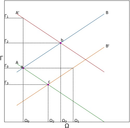
Macroeconomic and spatial general equilibrium (MSGE) are determined at point a where schedules A and B intersect. Faster population growth or technical progress shifts schedule A to A´. The new MSGE is at point b at which the rate if interest and Ω are larger (r₂ and Ω₃). If TFP in region 1 is larger than in region 2, a TFP shock in region 1 shifts schedule B to B´ at which the new equilibrium is at point c, at which the rate of interest is smaller and Ω is larger.

If equation (6b) is positive instead of negative, schedule A would slope downwards instead of upwards. If schedule A is flatter than schedule B, point b continues to lie north-east of point a as drawn. If schedule A is steeper than schedule B, point b would lie south-west of point a. If ψ happened to vary inversely with the rate of interest, schedule B would slope downwards instead of upwards as drawn. In general, schedules A and B may slope upwards or downwards, be steeper or flatter. This means that the taxonomy of MSGE is large.

A related result applies if rates of capital depreciation happen to vary between locations due for example, to meteorological or similar physical conditions. Equation (3c) becomes: (9) ${\displaystyle \frac{\kappa }{1-\kappa }={\left[{\displaystyle \frac{A_2}{A_1}{\left({\displaystyle \frac{1-\pi }{\pi }}\right)}^{1-\alpha }+{\displaystyle \frac{{\delta }_1-{\delta }_2}{\alpha A_1}{\left({\displaystyle \frac{1-\kappa }{\pi }}\right)}^{1-\alpha }}}\right]}^{{\displaystyle \frac{1}{\alpha -1}}}}$(9) If capital depreciates faster in region 2 than in region 1 (δ₂ > δ₁) region 1’s share of capital increases. Notice that if the rates of depreciation are the same, equation (9) reverts to equation (3c) as expected. Equation (9) implies that schedule B in Figure 1 is flat unless rates of depreciation vary with the rate of interest. Hence, the increase in n + a, which shifted schedule A to A´ in Figure 1 would not induce an increase in the rate of interest. On the other hand, a decrease in the rate of depreciation, which favoured location 1 (δ₁ – δ₂ decreases) would also induce a rightward shift in schedule B so that the MSGE would be determined by the intersection between schedules A´ and B´ at which the rate of interest would increase as drawn.

In summary, SGE and macroeconomic equilibrium are jointly determined. The rate of interest depends on SGE through Ω in equation (6a) when savings rates differ, and Ω depends on the rate of interest through equation (8b). If savings rates are the same, the rate of interest does not depend on SGE because equation (4d) applies instead of equation (6a), but SGE continues to depend on the rate of interest through equation (8b).

5. DISCUSSION

The present paper integrates SGE theory and macroeconomic theory. Since GDP is the sum of GRPs, there is an obvious link between the two bodies of theory. Beenstock (2020) explored some implications of SGE theory for aggregate supply, where the analysis was one way from economic geography to macroeconomics. The present paper complements the previous one in two main respects. First, it is two way: it explores the joint determination of SGE and macroeconomic equilibrium, and breaks the mutual dichotomy between economic geography and macroeconomics. Second, whereas there was no economic growth in the previous paper, the present paper integrates SGE theory with the theory of economic growth.

‘Macroeconomics’ is represented by the neoclassical growth model and ‘economic geography’ is represented by Roback (1982). Since both models are neoclassical and involve only one good, this marriage has intellectual appeal. Although the integrated model that results is very simple, it involves the key linkages between the spatial economy and the macroeconomy. Specifically, GDP and the rate of interest depend on SGE, and the spatial distribution of labour and capital depend on the rate of interest. The main results are as follows:

• If savings rates are spatially homogeneous and capital is perfectly mobile, the rate of interest is independent of SGE, but GDP is not.

• If capital mobility equates marginal products of capital, but regional savings rates are heterogeneous, both GDP and the rate of interest depend on SGE, but there is still no feedback from macroeconomics to SGE.

• If, marginal products of capital are not equated in equilibrium, GDP, the rate of interest and SGE are mutually dependent. Macroeconomic theory and SGE theory are mutually inseparable.

• The direction, however, is ambiguous depending on the correlation between regional savings rates and TFP. This result depends critically on the assumption that risk premia for the returns to capital vary directly with the rate of interest, as predicted by expected utility theory.

Although perfect internal capital mobility is a standard feature in SGE theory, empirical evidence suggests otherwise (Beenstock, 2017). Hence, the last result is empirically relevant.

Extending the number of locations beyond two complicates matters, but does not raise new conceptual issues. However, the ambiguity in the dependence of SGE on the rate of interest increases, depending on the correlation matrix between savings rates and TFP.

The analysis focuses on steady-state equilibria; it does not discuss transitional paths between equilibria, which is left for a separate occasion. Transitional dynamics in the neoclassical growth model have been widely studied, and transitional dynamics and multiple equilibria in SGE theory have been studied for the Roback model (Beenstock, 2020; Beenstock & Felsenstein, 2010) and for the NEG model (Brakman et al., 2009; Combes et al., 2008). We do not suspect that transitional dynamics in the integrated model should raise particular difficulties.

A related matter is that the analysis is entirely secular, partly because the integrated model is ‘real’ and partly because transitional dynamics have been ignored. A straightforward extension would be to introduce real business cycle theory (Romer, 2019) into the integrated model. Real business cycle theory is based on the idea that capital depreciates slowly and adjusting capital stocks is costly. In the present study relocation has been costless for labour as well as capital. Integrating RBC theory into present efforts by introducing frictions in labour as well as capital mobility would shed new light on the relation between business cycles and the spatial economy.

Another extension would be to introduce money and financial assets into the neoclassical growth model (Foley & Sidrausky, 1970; Johnson, 1967) so that real and nominal interest rates may be distinguished. A further extension would be to replace exogenous growth with endogenous growth, and to allow for spatial spillover in TFP shocks (Beenstock, 2020).

The NEG model serves as an alternative paradigm to Roback’s model. We have chosen Roback over NEG for several reasons. First, it is analytically tractable whereas NEG typically requires computer simulation (Brakman et al., 2009; Combes et al., 2008). Attempts to make NEG analytically tractable have been only partially successful, as noted in section 2. A marriage between Roback and the neoclassical growth model is more natural than one with NEG, since NEG involves multiple sectors, imperfect competition and frictions, which do not feature in the neoclassical growth model. The integration of macroeconomic theory with NEG requires a suitable macroeconomic partner such as the New Keynesian model (Romer, 2019; Walsh, 2017), which like NEG is based on the theory of imperfect competition and the New Theory of international trade. The driving force in the New Keynesian model is price stickiness, which by default, is assumed to be spatially homogeneous. A promising development, which would enrich New Keynesian business cycle theory, would be to allow price stickiness to be spatially heterogeneous.

6. CONCLUSIONS

Whereas macroeconomists have abstracted from economic geography by relating to space as a seamless whole, spatial economists have been unable to avoid macroeconomics because GDP is the sum of GRPs. On the other hand, they have been more concerned with studying the implications of spatial spillovers in knowledge for endogenous growth than engaging with macroeconomics proper, including savings and investment and the determination of the rate of interest. In the present paper I have tried to break this solipsism by integrating Roback’s ideas on SGE with the influential neoclassical growth model from macroeconomics. I have focused on the mutual relation between the rate of interest and the spatial distribution of economic activity. Thus far, it has been easier to relate macroeconomics to SGE than the other way around. The latter requires introducing imperfect capital mobility across space in a way that depends on the rate of interest.

The sine qua non for integrating macroeconomics and SGE theory include internal labour mobility and capital mobility as well, of course, internal trade. Labour, capital and goods markets lie at the heart of macroeconomics. So, do financial and money markets, which have been ignored here. Hence, the present study has been concerned with ‘real’ theory rather than ‘monetary’ theory. For this reason, the focus has been limited to secular theory rather than business cycle theory. Also, it has referred to a closed economy; so, there is no exchange rate or balance of payments. Nor has there been a government or a central bank. These omissions have been made to get started in the belief that one begins with the basics of the real economy before moving on. Obviously, much remains to be done.

DISCLOSURE STATEMENT

No potential conflict of interest was reported by the author.

REFERENCES

- Baldwin, R., & Forslid, R. (2000). The core–periphery model and endogenous growth: Stabilizing and destabilizing integration. Economica, 67(267), 307–324. https://doi.org/10.1111/1468-0335.00211
- Baldwin, R., Forslid, R., Martin, P., Ottaviano, G., & Robert-Nicoud, F. (2003). Economic geography and public policy. Princeton University Press.
- Baldwin, R., & Martin, P. (2004). Agglomeration and growth. In V. Henderson & J. Thisse (Eds.), The handbook of regional and urban economics (Vol. 6, pp. 2671–2712). Amsterdam: Elsevier.
- Barro, R. J., & Sala-i-Martin, X. (2004). Economic growth. MIT Press.
- Beenstock, M. (2017). How internally mobile is capital? Letters in Spatial and Resource Science, 10(3), 361–374. https://doi.org/10.1007/s12076-017-0190-1
- Beenstock, M. (2020). Aggregate supply in spatial general equilibrium. Spatial Economic Analysis, 15(4), 374–391. https://doi.org/10.1080/17421772.2020.1742928
- Beenstock, M. (2021). Macroeconomics meets regional science: How national economic activity is related to regional economic activity. International Regional Science Review. https://doi.org/10.1177/01600172611034140
- Beenstock, M., & Felsenstein, D. (2010). Marshallian theory of agglomeration. Papers in Regional Science, 89(1), 155–172. https://doi.org/10.1111/j.1435-5957.2009.00253.x
- Bond-Smith, S. (2021). The unintended consequences of increasing returns to scale in geographical economics. Journal of Economic Geography, 21(5), 653–681. https://doi.org/10.1093/jeg/lbab023
- Bond-Smith, S., & McCann, P. (2020). A multisector model of relatedness, growth and industry clustering. Journal of Economic Geography, 20(5), 1145–1163. https://doi.org/10.1093/jeg/lbz031
- Bond-Smith, S., McCann, P., & Oxley, L. (2018). A regional model of endogenous growth without scale effects. Spatial Economic Analysis, 13(1), 5–35. https://doi.org/10.1080/17421772.2018.1392038
- Brakman, S., Garretsen, H., & Van Marrewijk, C. (2009). The New introduction to geographical economics (2nd ed.). Cambridge University Press.
- Combes, P.-P., Mayer, T., & Thisse, J.-F. (2008). Economic geography: The integration of regions and nations. Princeton University Press.
- Davis, C. R. (2009). Interregional knowledge spillovers and occupational choice in a model of free trade and endogenous growth. Journal of Regional Science, 49(5), 855–876. https://doi.org/10.1111/j.1467-9787.2009.00612.x
- Davis, C. R., & Hashimoto, K.-I. (2014). Patterns of technology, industry concentration and productivity growth without scale effects. Journal of Economic Dynamics and Control, 40, 266–278. https://doi.org/10.1016/j.jedc.2014.01.010
- Davis, C. R., & Hashimoto, K.-I. (2015). Industry concentration, knowledge diffusion and economic growth without scale effects. Economica, 82(328), 769–789. https://doi.org/10.1111/ecca.12129
- Foley, D., & Sidrausky, M. (1970). Portfolio choice, investment and growth. American Economic Review, 60, 44–63.
- Forslid, R., & Ottaviano, G. (2003). An analytically solvable core–periphery model. Journal of Economic Geography, 3(3), 229–240. https://doi.org/10.1093/jeg/3.3.229
- Greene, W. A. (2012). Econometric analysis (7th ed.). Pearson.
- Harris, R. (2011). Models of regional growth: Past, present and future. Journal of Economic Surveys, 25(5), 913–951. https://doi.org/10.1111/j.1467-6419.2010.00630.x
- Hicks, J. R. (1932). The theory of wages. Macmillan.
- Johnson, H. G. (1967). Money in a neoclassical one-sector growth model. Essays in monetary economics. Allen and Unwin.
- Jones, C. I. (1995). R&D based models of economic growth. Journal of Political Economy, 103(4), 759–784. https://doi.org/10.1086/262002
- Kichko, S. (2018). Trade costs, regional inequality and the home market effect. Spatial Economic Analysis, 13(4), 387–399. https://doi.org/10.1080/17421772.2018.1500026
- Krugman, P. (1991). Geography and trade. MIT Press.
- Maddala, G. S. (1983). Limited-dependent variables and qualitative variables in econometrics. Cambridge University Press.
- Peretto, F. P. (1998). Technological change and population growth. Journal of Economic Growth, 3(4), 283–311. https://doi.org/10.1023/A:1009799405456
- Ramsey, F P. (1928). A mathematical theory of saving. The Economic Journal, 38, 543–559.
- Rappaport, J. (2004). Why are population flows so persistent? Journal of Urban Economics, 56(3), 554–580. https://doi.org/10.1016/j.jue.2004.07.002
- Roback, J. (1982). Wages, rents and the quality of life. Journal of Political Economy, 90(6), 1257–1278. https://doi.org/10.1086/261120
- Romer, D. (2019). Advanced macroeconomics (5th ed.). McGraw Hill.
- Walsh, C. E. (2017). Monetary theory and policy (4th ed.). MIT Press.
- Yamamoto, K. (2003). Agglomeration and growth with innovation in the intermediate goods sector. Regional Science and Urban Economics, 33(3), 335–360. https://doi.org/10.1016/S0166-0462(02)00032-7
- Young, A. (1998). Growth without scale effects. Journal of Political Economy, 106(1), 41–63. https://doi.org/10.1086/250002