The social footprint of globalisation: towards the introduction of strategic industries in quantitative trade models

ABSTRACT

We argue that our understanding of industrial policy in the presence of ‘strategic’ industries that exert positive externalities on the national economy may benefit from an extension of quantitative general equilibrium trade models making the extent and pattern of trade-induced reallocations more salient. To make these features relevant for national welfare, we introduce the notion of the ‘social footprint’ of globalisation as the result of suboptimal trade-induced structural transformation in the presence of externalities. For proof of concept, we use simple workhorse models featuring two countries and two industries (only one of which is ‘strategic’) to highlight the role of the ‘scale elasticity’ of the strategic industry and the consequences of the most common assumptions on market structure in quantitative trade analyses.

KEYWORDS:

• Globalisation
• quantitative trade models
• trade liberalisation
• market structure
• externalities
• strategic industries

JEL:

• F11
• F12
• F17
• F15
• F62

1. INTRODUCTION

Industrial policy has become a priority for Western governments. In May 2021 the European Union updated the industrial strategy it had unveiled the previous year with the aim of supporting the twin green and digital transitions, making EU industry more competitive globally, and enhancing Europe’s open strategic autonomy. The European approach emphasises government intervention in strategic areas in order ‘to develop activities that would not develop otherwise’,¹ such as those concerning processors and semiconductor technologies. In September 2022, on the other side of the pond, the US Department of Commerce unveiled its plan to spend 50 billion dollars of taxpayer money to scale up the American semiconductor industry, arguably the US’s biggest effort to shape a strategic industry as well as its most significant investment in industrial policy in at least fifty years.

The economic weight of the countries involved and the sheer amount of money committed will likely have seismic consequences beyond the targeted industries, both at home and abroad. To understand and evaluate such local and global consequences of industrial policy, traditional partial equilibrium models of industrial organisation should be complemented with general equilibrium mechanisms operating both within and across country borders. In this respect, new quantitative models recently introduced in the field of international trade (see, e.g., Costinot & Rodríguez-Clare, 2014) hold a lot of promise. The aim of this paper is to discuss how their potential could be developed, expanding on the discussion on the backlash of globalisation in Colantone et al. (2022).

New quantitative trade models combine features borrowed from Armington (1969), Krugman (1980), Eaton and Kortum (2002) and Melitz (2003). They rely on four common primitive assumptions, which are Dixit-Stiglitz preferences, one factor of production, linear cost functions, and perfect or monopolistic competition. They also comply with three common aggregate restrictions, requiring trade to be balanced, aggregate profits to be a constant share of aggregate revenues and the import demand system to exhibit constant elasticity of substitution (CES). Calibrated with several countries, several sectors and rich input-output linkages, they have been applied to quantify how trade policy shocks affect national welfare, usually measured as per-capita real consumption or expenditures (Caliendo & Parro, 2022).²

Current versions of those models exhibit, however, three main limitations with respect to the analysis of industrial policy. First, for practical purposes, trade scholars have been driven by the desire to identify as few as possible sufficient statistics in order to reduce the amount of information needed for the quantitative assessment of the welfare effects of enacted or counterfactual policies. This has led them to look more at the similarities between the implications of different modelling assumptions than at their differences. From the perspective of industrial policy, an important example of the unintended consequences of such a reductionist approach is the conventional wisdom that assuming perfect or monopolistic competition has no qualitative, and at most only small quantitative implications for the analysis. Second, the CES assumption implies that the market outcome is efficient not only with perfect competition, but also with monopolistic competition at least within industries, while between industries the extent of market inefficiency is regulated only by differences in the elasticity of substitution, which is an unlikely industrial policy parameter. Third, there is no way some industries can be singled out as ‘strategic’. Consider, for example, the effects of trade liberalisation, which is the most studied type of policy intervention. While trade liberalisation generates gains from trade arising from more efficient specialisation in production, richer product variety and tougher firm selection, the extent and the pattern of the implied trade-induced intersectoral reallocations of resources are inconsequential, as trade liberalisation increases national welfare independently of the resulting industry specialisation. In this respect, the notion of ‘strategic’ industry is immaterial and thus necessarily left out of the picture.

To overcome those limitations, we propose to operationalise the notion of strategic industry in a way that can be readily introduced in the quantitative trade models, making its concrete relevance an empirical issue linked to the estimation of an industry scale parameter conditional on the choice of industry market structure. This is achieved by defining as ‘strategic’ for a country an industry that generates positive nation-wide externalities, that is, unpriced costs and benefits to national welfare arising as effects of its activity. Being unpriced, such costs and benefits do not enter the individual decisions of households and firms, which drives a wedge between private and social evaluations and thus justifies policy action to realign them.

For ease of comparison with the trade literature, we then investigate the effects of trade liberalisation and study specifically how it affects the welfare consequences of the wedge between private and social incentives. We call these consequences the ‘social footprint of globalisation’ as permanent suboptimal results for society of the trade-induced structural transformation in the presence of externalities. For proof of concept, our investigation relies on simple workhorse versions of the models by Armington (1969), Krugman (1980), Eaton and Kortum (2002) and Melitz (2003), featuring two industries, one of which is strategic, and two countries, one of which has a locational advantage in the strategic industry. We compare two types of locational advantage (comparative advantage and market access) and the two types of market structure (perfect competition and monopolistic competition). In all cases, as trade gets freer, the strategic industry relocates from the country with a locational disadvantage to the country with a locational advantage. Due to the positive externality characterising the strategic industry, such relocation reduces the welfare gains from trade in the former country and amplifies them in the latter. However, with perfect competition in the strategic industry, the country where that industry shrinks suffers less from the weakened externality if trade liberalisation is deeper, whereas with monopolistic competition it suffers less if trade liberalisation in shallower. The reason for such asymmetry is that under monopolistic competition structural transformation gains momentum as trade gets freer, whereas the opposite happens under perfect competition. This shows that the way in which market structure is modelled may matter much more than generally understood in the literature on quantitative trade models.

The rest of the paper is organised as follows. Section 2 presents the main features of the workhorse models, highlighting their common and exclusive features. Section 3 activates the externality in the strategic industry and introduces the notion of ‘social footprint’ of globalisation by showing how trade gains may come together with trade pains. Section 4 derives and compares the welfare effects of trade liberalisation across models highlighting the role of the strategic sector’s scale elasticity. Section 5 concludes.

2. WORKHORSE MODELS

The most popular trade models used for quantitative analysis are those put forth by Armington (1969), Krugman (1980), Eaton and Kortum (2002) and Melitz (2003). In recent years, through the sufficient statistics approach of Arkolakis et al. (2012), various combinations of these models have been calibrated and used to structurally quantify the general equilibrium effects of both factual and counterfactual trade-related shocks – including the North American free trade agreement (NAFTA) (Caliendo & Parro, 2015), Brexit (Dhingra et al., 2017) and the rise of China as global actor (Caliendo et al., 2019) – for which standard econometric approaches are of limited use due to lack of data. These quantitative applications consider many sectors and regions connected by complex networks of input-output relations. Yet, for our purposes, it is more useful to follow Colantone et al. (2022) and rely on simpler, but more analytically transparent versions featuring two countries, two sectors and one productive factor only.

We call the two countries $H$ (‘home’) and $F$ (‘foreign’) and assume that they are inhabited by fixed ‘numbers’ of consumers/workers $L_H$ and $L_F$. Each worker supplies one unit of labour inelastically so that $L_H$ and $L_F$ are also the countries’ labour endowments. We focus on country $H$, with symmetric expressions holding for country $F$. The two sectors are designed so that, in terms of national welfare, the international distribution of production is important for a sector but irrelevant for the other. We bring the former sector to the forefront, dubbing it ‘strategic’ for the sake of brevity and using $L_H^d$ and $L_F^d$ to denote country $H$’s and country $F$’s employment in that sector. The reason why its international distribution matters is that the strategic sector generates a positive nation-wide externality.

2.1. Common features

The preferences of the representative consumer are captured by the nested Cobb–Douglas CES utility function, (1) $U_H^c=B_H(Q_H^c{)}^{\alpha }(O_H^c{)}^{1-\alpha },$(1) with upper-tier CES quantity index, (2) $Q_H^c={\left[{(Q_{\mathrm{HH}}^c)}^{\frac{\sigma -1}{\sigma }}+{(Q_{\mathrm{FH}}^c)}^{\frac{\sigma -1}{\sigma }}\right]}^{\frac{\sigma }{\sigma -1}},$(2) and lower-tier CES quantity indexes, (3) $\begin{array}{ccc}{Q}_{\mathrm{HH}}^c& ={\left[{\int }_0^{N_H}{(q_{\mathrm{HH}}^c(\omega ))}^{\frac{\sigma -1}{\sigma }}\mathrm{d\omega }\right]}^{\frac{\sigma }{\sigma -1}},& \\ Q_{\mathrm{FH}}^c& ={\left[{\int }_0^{N_F}{(q_{\mathrm{FH}}^c(\omega ))}^{\frac{\sigma -1}{\sigma }}\mathrm{d\omega }\right]}^{\frac{\sigma }{\sigma -1}}.& \end{array}$(3) Where $B_H=(L_H^d{)}^{\gamma }$, with scale elasticity $\gamma >0$, is the positive nation-wide externality arising from employment in the strategic sector, $Q_H^c$ is consumption of a basket of home and foreign produced varieties of a horizontally differentiated good, $Q_{\mathrm{HH}}^c$ ($Q_{\mathrm{FH}}^c$) is consumption of the sub-basket of $N_H$ ($N_F$) home (foreign) produced varieties, and $q_{\mathrm{HH}}^c(\omega )$ ($q_{\mathrm{FH}}^c(\omega )$) is consumption of home (foreign) produced varieties. As for $O_H^c$, this is consumption of a homogeneous good (‘outside good’). Parameters satisfy the restrictions $\alpha \in (0,1)$ and $\sigma >1$ so that varieties are more substitutable with one another than with the outside good. Different models activate different tiers. $B_H$ can be equivalently interpreted as a consumption externality or a production externality given that (1) can also represent the aggregate production function for a final, non-tradable, good that enters utility linearly. In standard quantitative trade models there is no such externality: $\gamma =0$ and thus $B_H=1$ hold.

Basket $Q_H^c$ as well as sub-baskets $Q_{\mathrm{HH}}^c$ and $Q_{\mathrm{FH}}^c$ have associated exact price indices, (4) $P_H=[{(P_{\mathrm{HH}})}^{1-\sigma }+{(P_{\mathrm{FH}})}^{1-\sigma }{]}^{\frac{1}{1-\sigma }}$(4) for the upper tier and (5) $\begin{array}{ccc}{P}_{\mathrm{HH}}& ={\left[{\int }_0^{N_H}{(p_{\mathrm{HH}}(\omega ))}^{1-\sigma }\mathrm{d\omega }\right]}^{\frac{1}{1-\sigma }},& \\ P_{\mathrm{FH}}& ={\left[{\int }_0^{N_F}{(p_{\mathrm{FH}}(\omega ))}^{1-\sigma }\mathrm{d\omega }\right]}^{\frac{1}{1-\sigma }},& \end{array}$(5) for the lower tier, where $p_{\mathrm{HH}}(\omega )$ and $p_{\mathrm{FH}}(\omega )$ are the delivered prices of home and foreign produced varieties. Hence, using $E^c$ to denote consumer expenditure, the consumer constraint can be stated as, (6) $P_H{Q}_H^c+P_H^o{O}_H^c=P_{\mathrm{HH}}{Q}_{\mathrm{HH}}^c+P_{\mathrm{FH}}{Q}_{\mathrm{FH}}^c+P_H^o{O}_H^c=E^c$(6) where $P_H^o$ is the delivered price of the outside good.

Denoting aggregate consumption levels by $Q_{\mathrm{HH}}=Q_{\mathrm{HH}}^c{L}_H$, $Q_{\mathrm{FH}}=Q_{\mathrm{FH}}^c{L}_H$, $Q_H=Q_H^c{L}_H$ and $O_H=O_H^c{L}_H$, maximisation of utility (1) subject to the budget constraint (6) implies that aggregate expenditure $E_H=E_H^c{L}_H$ is split between the differentiated basket and the outside good according to $\alpha E_H=P_H{Q}_H$ and $(1-\alpha )E_H=P_H^o{O}_H^c$ respectively. Indirect utility can then be rewritten as $W_H=B_H{V}_H$ with real consumption (or expenditure) per capita as (7) $V_H={\alpha }^{\alpha }(1-\alpha {)}^{1-\alpha }{\displaystyle \frac{E_H/L_H}{{(P_H)}^{\alpha }{(P_H^o)}^{1-\alpha }}.}$(7) The markets for labour and the outside good are perfectly competitive while the market of the differentiated good is either perfectly or monopolistically competitive depending on the models. Free entry then implies that expenditure equals labour income: (8) $E_H=w_H{L}_H$(8) where $w_H$ is the wage.

The outside good is produced employing $1$ unit of labour per unit of output so that its marginal cost is equal to the wage. This good is freely traded and chosen as numeraire, implying that its price is the same in both countries: $P_H^O=P_F^O=P^O=1$. Moreover, as profit is maximised by marginal cost pricing ($P^O=w_H=w_F$), also wages are equalised across countries: $w_H=w_F=w=1$. Wage equalisation holds as long as both countries produce the outside good, which happens when neither country on its own can supply world demand for that good even if fully specialised in its supply. This is the case when condition $\alpha <min\left[{\displaystyle \frac{L_H}{L_H+L_F},{\displaystyle \frac{L_F}{L_H+L_F}}}\right]$holds, which we assume henceforth. Designing the outside good sector this way vastly simplifies the analysis.

In equilibrium, market clearing requires that a country’s labour income from the differentiated varieties equals the world’s expenditures on those varieties, (9) $L_H^d={\lambda }_{\mathrm{HH}}\alpha L_H+{\lambda }_{\mathrm{HF}}\alpha L_F,$(9) where ${\lambda }_{\mathrm{HH}}$ and ${\lambda }_{\mathrm{HF}}$ are the shares of domestic and foreign expenditures on country $H$’s varieties such that ${\lambda }_{\mathrm{HH}}={\left({\displaystyle \frac{P_{\mathrm{HH}}}{P_H}}\right)}^{1-\sigma }\mathrm{and}{\lambda }_{\mathrm{HF}}={\left({\displaystyle \frac{P_{\mathrm{HF}}}{P_F}}\right)}^{1-\sigma }.$

Then, price and wage equalisation $P_H^O=w_H=1$ allows us to rewrite real consumption (7) as (10) $V_H={\alpha }^{\alpha }(1-\alpha {)}^{1-\alpha }(P_{\mathrm{HH}}{)}^{-\alpha }({\lambda }_{\mathrm{HH}}{)}^{-\frac{\alpha }{\sigma -1}}.$(10) When there is no externality from the strategic industry to the national economy, $\gamma =0$ and thus $B_H=1$ hold so that real consumption and indirect utility coincide ($W_H=V_H$). Otherwise for $\gamma >0$, and thus $B_H\ne 1$, $W_H=B_H{V}_H$ implies that indirect utility evaluates to: (11) $W_H={\alpha }^{\alpha }(1-\alpha {)}^{1-\alpha }{B}_H(P_{\mathrm{HH}}{)}^{-\alpha }({\lambda }_{\mathrm{HH}}{)}^{-\frac{\alpha }{\sigma -1}}.$(11) which we take as our measure of national welfare.

2.2. Exclusive features

Beyond their common features, the simplified versions of the four most popular trade models can be divided into two pairs according to their specific assumptions on the production technologies of the differentiated varieties and the corresponding market structures.

2.2.1. Constant returns to scale and perfect competition

Constant-return technologies and perfectly competitive market structures characterise the models by Armington (1969) and Eaton and Kortum (2002). In Armington (1969) only the upper-tier basket (2) is activated with $c_H$ and $c_F$ units of labour required per unit of output. International shipments incur iceberg trade costs such that τ $>1$ units have to be shipped for one unit to reach its destination. Country $H$ is always the lowest price supplier of the home produced sub-basket everywhere, with prices set at delivered marginal cost $P_{\mathrm{HH}}=c_H$ and $P_{\mathrm{HF}}=$ τ$P_{\mathrm{HH}}$. Country $F$ is always the lowest price supplier everywhere of the foreign produced sub-basket, with prices set at delivered marginal cost $P_{\mathrm{FF}}=c_F$ and $P_{\mathrm{FH}}=$ τ$P_{\mathrm{FF}}$. Given the upper-tier CES basket (2), expenditure shares evaluate to (12) $\begin{array}{ccc}{\lambda }_{\mathrm{HH}}& ={\displaystyle \frac{{(P_{\mathrm{HH}})}^{1-\sigma }}{{(P_{\mathrm{HH}})}^{1-\sigma }+{(P_{\mathrm{FH}})}^{1-\sigma }}={\displaystyle \frac{a}{a+\varphi },}}& \\ {\lambda }_{\mathrm{HF}}& ={\displaystyle \frac{{(P_{\mathrm{HF}})}^{1-\sigma }}{{(P_{\mathrm{HF}})}^{1-\sigma }+{(P_{\mathrm{FF}})}^{1-\sigma }}={\displaystyle \frac{\mathrm{a\varphi }}{1+\mathrm{a\varphi }},}}& \end{array}$(12) where $a=(c_F/c_H{)}^{\sigma -1}$ measures country $H$’s comparative advantage ($a>1$) or disadvantage ($a<1$) in the production of the differentiated good (as the outside good’s unit labour requirement is the same in the two countries) and $\varphi =$ τ${}^{1-\sigma }\in [0,1]$ measures the freeness of trade, with $\varphi =0$and $\varphi =1$ corresponding to autarky and free trade respectively. Hence, in autarky we have ${\lambda }_{\mathrm{HH}}=1$ and ${\lambda }_{\mathrm{HF}}=0$. Together with market clearing (9) and analogous expressions for country $F$, shares (12) imply that equilibrium employment in ‘strategic’ differentiated production evaluates to (13) $L_H^d=\alpha L_H-{\displaystyle \frac{\varphi }{a+\varphi }\alpha (L_H-L_F)+{\displaystyle \frac{\varphi (a^2-1)}{(a+\varphi )(1+\mathrm{a\varphi })}\alpha L_F.}}$(13) This expression shows that in autarky ($\varphi =0$) differentiated employment equals a share $\alpha$ of the workforce, as the country spends a share $\alpha$ of its income on the differentiated basket and the basket has to be entirely supplied domestically. Otherwise ($\varphi \in (0,1]$), differentiated employment deviates from its autarkic level due to two forces: differences in market size ($L_H\ne L_F$) and comparative advantage ($a\ne 1$). In particular, we have $L_H^d>\alpha L_H$ if, relative to autarky, lost domestic demand is more than compensated by gained foreign demand, that is, if comparative advantage ($a>1$) is strong enough or the size advantage of the foreign market ($L_F/L_H>1$) is large enough.³ When that is the case, we say that country $H$ has a locational advantage in the strategic industry.

Expression (13) reveals what we may call a ‘reverse home market effect’: without comparative advantage ($a=1$), the larger country is an importer of the differentiated basket. Sectoral specialisation is always incomplete as (13) implies $L_H^d>0$ and an analogous expression for country $F$ implies $L_F^d>0$. Intuitively, this derives from the fact that each country is always the lowest price supplier everywhere of its own sub-basket. Finally, larger $\varphi$ reinforces the effects of both market size asymmetry and comparative advantage.

Given (10), marginal cost pricing $P_{\mathrm{HH}}=c_H$ and expenditure share (12) imply that the ratio of real consumption with trade freeness $\varphi$ to real consumption with ${\varphi }^{\mathrm{\prime }}$ evaluates to: (14) ${\displaystyle \frac{V_H(\varphi )}{V_H({\varphi }^{\mathrm{\prime }})}={\left({\displaystyle \frac{{\lambda }_{\mathrm{HH}}(\varphi )}{{\lambda }_{\mathrm{HH}}({\varphi }^{\mathrm{\prime }})}}\right)}^{-\frac{\alpha }{\epsilon }},}$(14) where $\epsilon =\sigma -1$ is the trade elasticity, which by (12) measures the percentage fall in bilateral trade for a one percent increase in the iceberg cost controlling for origin and destination characteristics (Head & Mayer, 2014).

Differently from Armington (1969), Eaton and Kortum (2002) also activate the lower-tier sub-baskets (3) with fixed $N_H=N_F=1$. Moreover, which country is the lowest price supplier of either sub-basket is uncertain. Specifically, country $H$ has probability $(c_H{)}^{-\theta }/[{(c_H)}^{-\theta }+{(c_F)}^{-\theta }$ τ${}^{-\theta }]$ to be the lowest price supplier of any variety to $H$ as delivered prices at marginal cost $P_{\mathrm{HH}}=c_H$ and $P_{\mathrm{HF}}=$ τ$P_{\mathrm{HH}}$ are determined by a random unit labour requirement $c=1/z$, with efficiency $z$ drawn from a Fréchet (or extreme value) distribution with cumulative density function: $F_H(z)=e^{-{(c_{H}z)}^{-\theta }}\mathrm{for}z\in [0,\mathrm{\infty }),$where $c_H>0$ is the scale parameter (larger $c_H$ shifts density towards the lower bound of the support, making higher efficiency draws less likely) and $\theta >0$ is the shape parameter (larger $\theta$ reduces the heterogeneity of efficiency draws around the mode of the distribution). Analogous expressions hold for country $F$. Yet, the equilibrium expenditure shares, differentiated employment and relative real consumption are still given by (12), (13) and (14) respectively, the only difference with respect to Armington (1969) being that the trade elasticity $\epsilon =\theta$ is now determined by the heterogeneity of efficiency draws rather than the elasticity of substitution. Specialisation is also always incomplete in Eaton and Kortum (2002) as both countries always have a positive probability of being the lowest price supplier of each lower-tier sub-basket.

2.2.2. Monopolistic competition and increasing returns to scale

Increasing-return technologies and monopolistically competitive market structure characterise the models by Krugman (1980) and Melitz (2003). As in Eaton and Kortum (2002) but differently from Armington (1969), both models also activate the lower-tier sub-baskets (3). However, differently from Eaton and Kortum (2002), the numbers of varieties of $N_H$ and $N_F$ are endogenous due to free entry and each variety is produced by a monopolistically competitive firm under increasing returns to scale, rather than by a mass of perfectly competitive firms under constant returns to scale. Moreover, while in Krugman (1980), as in Armington (1969), there is no ex-ante uncertainty about efficiency in production, in Melitz (2003), as in Eaton and Kortum (2002), uncertainty is there.

In Krugman (1980), increasing returns at the firm level derive from the presence of a fixed labour requirement for production. Specifically, supplying $q$ units of output requires ${\ell }_H(q)=f+c_{H}q$ units of labour. International shipments of the differentiated varieties again incur iceberg trade costs such that τ $>1$ units have to be shipped for one unit to reach its destination. Varieties are priced at constant markup $\sigma /(\sigma -1)$ over delivered marginal cost (‘mill pricing’). Using ${\tilde{p}}_{\mathrm{HH}}$ to denote the mill price, we have ${\tilde{p}}_{\mathrm{HH}}=c_H\sigma /(\sigma -1)$ and ${\tilde{p}}_{\mathrm{HF}}=$ τ${\tilde{p}}_{\mathrm{HH}}$. Zero profit, due to free entry, then implies that all firms operate at the same scale, $q_H=f(\sigma -1)/c_H$, so that they also share the same employment level, ${\ell }_H=\mathrm{f\sigma }$. The number of firms is therefore a linear function of total employment in the differentiated goods sector: $N_H=L_H^d/(\mathrm{f\sigma })$. Hence, given sub-baskets (2) and (3), expenditure shares evaluate to: (15) $\begin{array}{ccc}{\lambda }_{\mathrm{HH}}& =& {\displaystyle \frac{N_H{({\tilde{p}}_{\mathrm{HH}})}^{1-\sigma }}{N_H{({\tilde{p}}_{\mathrm{HH}})}^{1-\sigma }+N_F{({\tilde{p}}_{\mathrm{FH}})}^{1-\sigma }}={\displaystyle \frac{a{L}_H^d}{a{L}_H^d+\varphi L_F^d},}}\\ {\lambda }_{\mathrm{HF}}& =& {\displaystyle \frac{N_H{({\tilde{p}}_{\mathrm{HF}})}^{1-\sigma }}{N_H{({\tilde{p}}_{\mathrm{HF}})}^{1-\sigma }+N_F{({\tilde{p}}_{\mathrm{FF}})}^{1-\sigma }}={\displaystyle \frac{\mathrm{\varphi a}{L}_H^d}{\mathrm{\varphi a}{L}_H^d+L_F^d},}}\end{array}$(15) as we have $(P_{\mathrm{HH}}{)}^{1-\sigma }=N_H({\tilde{p}}_{\mathrm{HH}}{)}^{1-\sigma }$ and $(P_{\mathrm{HF}}{)}^{1-\sigma }=N_F({\tilde{p}}_{\mathrm{FH}}{)}^{1-\sigma }$. Together with market clearing (9) and analogous expressions for country $F$, (15) shares imply that equilibrium employment in ‘strategic’ differentiated production equals: (16) $L_H^d=\alpha L_H+{\displaystyle \frac{\mathrm{a\varphi }}{1-\mathrm{a\varphi }}\alpha (L_H-L_F)+{\displaystyle \frac{\varphi (a^2-1)}{(a-\varphi )(1-\mathrm{a\varphi })}\alpha L_F.}}$(16)

This expression shows that in autarky ($\varphi =0$), differentiated employment is again equal to a share $\alpha$ of the workforce. Otherwise ($\varphi \in (0,1]$), as in the case of perfect competition, differentiated employment deviates from its autarkic level due to two forces: differences in market size ($L_H\ne L_F$) and comparative advantage ($a\ne 1$). In particular, we have $L_H^d>\alpha L_H$ if, relative to autarky, domestic demand grows relative to foreign demand, which happens if the domestic price index falls more than the foreign one, that is, if comparative advantage ($a>1$) is strong enough or the home market ($L_H/L_F>1$) is large enough.⁴ When this is the case we say, as before, that country $H$ has a locational advantage in the strategic industry.

Differently from the case of perfect competition, there is what Krugman (1980) calls a ‘home market effect’: without comparative advantage ($a=1$), the larger country is an exporter of the differentiated basket. Incomplete sectoral specialisation requires $L_H^d>0$ and $L_F^d>0$, which is the case if asymmetries between countries in technology as well as market size are not too large and the degree of trade freeness is not too high: (17) $\varphi {\displaystyle \frac{a-\varphi }{1-\mathrm{a\varphi }}<{\displaystyle \frac{L_F}{L_H}<{\displaystyle \frac{1}{\varphi }{\displaystyle \frac{a-\varphi }{1-\mathrm{a\varphi }},}}}}$(17) with necessary condition $(a-\varphi )/(1-\mathrm{a\varphi })>0$, that is, $\varphi <a<1/a$ if $a<1$ and $\varphi <1/a<a$ if $a>1$. Finally, when (17) holds, (16) also shows that, as with perfect competition, larger $\varphi$ reinforces the effects of both market size and technology asymmetries. However, compared with perfect competition, reinforcement is stronger in the case of comparative advantage and also, in the case of size asymmetries, for $a>(1-\varphi )/(1+\varphi )$.

Together with analogous expressions for country $F$, ${\tilde{p}}_{\mathrm{HH}}=c_H\sigma /(\sigma -1)$, ${\tilde{p}}_{\mathrm{HF}}=$ τ${\tilde{p}}_{\mathrm{HH}}$, $N_H=L_H^d/(\mathrm{f\sigma })$, (5) and (16) allow us to write the ratio of real consumption with trade freeness $\varphi$ to real consumption with trade freeness ${\varphi }^{\mathrm{\prime }}$ as (18) ${\displaystyle \frac{V_H(\varphi )}{V_H({\varphi }^{\mathrm{\prime }})}={\left({\displaystyle \frac{L_H^d({\varphi }^{\mathrm{\prime }})}{L_H^d(\varphi )}{\displaystyle \frac{{\lambda }_{\mathrm{HH}}(\varphi )}{{\lambda }_{\mathrm{HH}}({\varphi }^{\mathrm{\prime }})}}}\right)}^{-\frac{\alpha }{\epsilon }},}$(18) where $\epsilon =\sigma -1$ is again the trade elasticity. Comparing (18) with (14) shows that, unlike with perfect competition, monopolistic competition employment in the strategic sector matters for real consumption beyond its implicit relevance through the domestic expenditure share. This, together with the different behaviour of $L_H^d$ as a function of $\varphi$ in (13) and (16), implies a negative correlation of welfare gains across countries between market structures (Colantone et al., 2022). That is, countries that witness relatively higher welfare gains (or lower losses) under perfect competition tend to display relatively lower welfare gains (or higher losses) under monopolistic competition.

Differently from Krugman (1980), in Melitz (2003) firms enter the market under a veil of ignorance about their efficiency. They are thus ex-ante identical but ex-post heterogeneous as in Eaton and Kortum (2002). However, while in Eaton and Kortum (2002) many firms with the same efficiency supply any given variety, in Melitz (2003) as in Krugman (1980) only one firm supplies such variety. Specifically, in Melitz (2003) a firm incurs a sunk labour requirement $f_e$ to enter the market. By hiring $f_e$ workers the firm invents its own variety and discovers its efficiency $z=1/c$ in supplying it. Production of $q$ units of output then requires $f+\mathrm{cq}$ units of labour, as in Krugman (1980). Efficiency $z$ is unknown to the firm before paying $f_e$ and, upon entry, it is drawn from a Pareto distribution with scale parameter $1/c_H$ and shape parameter $\theta \ge 1$. This implies that the unit labour requirement $c$ is itself determined as the realisation of a random variable with cumulative density function, (19) $G_H(c)={\left({\displaystyle \frac{c}{c_H}}\right)}^{\theta }\mathrm{for}c\in [0,c_H].$(19) While larger $c_H$ makes higher efficiency draws less likely, larger $\theta$ reduces the heterogeneity of efficiency draws away from the mode $c_H$. Exporting incurs not only an iceberg trade cost τ $>1$ but also a fixed export cost $f_x=f$.

Ex ante, an entrant expects to sell a variety in the domestic and foreign markets with probabilities $(c_{\mathrm{HH}}/c_H{)}^{\theta }$ and τ${}^{-\theta }(c_{\mathrm{FF}}/c_H{)}^{\theta }$ respectively. Ex post, these probabilities translate into the fractions of entrants that produce and of entrants that export. This is due to the law of large numbers and holds for the ex-ante expected and ex-post average values of all variables. Varieties produced are priced on average at constant markup over expected delivered marginal costs ${\tilde{p}}_{\mathrm{HH}}=\frac{\sigma }{\sigma -1}{\tilde{c}}_H$ and ${\tilde{p}}_{\mathrm{HF}}=$ τ${\tilde{p}}_{\mathrm{HH}}$ with (20) ${\tilde{c}}_H={\left[{\int }_0^{c_{\mathrm{HH}}}{c}^{1-\sigma }d{\left({\displaystyle \frac{c}{c_{\mathrm{HH}}}}\right)}^{\theta }\right]}^{\frac{1}{1-\sigma }}={\displaystyle \frac{\theta }{\theta -\sigma +1}{c}_{\mathrm{HH}},}$(20) where $c_{\mathrm{HH}}$ is the domestic cutoff marginal cost corresponding to zero domestic demand, (21) $c_{\mathrm{HH}}={\left[{\displaystyle \frac{f_e}{f}{\displaystyle \frac{\theta -\sigma +1}{\sigma -1}{\displaystyle \frac{1-\varphi {\left({\displaystyle \frac{c_F}{c_H}}\right)}^{\theta }}{1-{\varphi }^2}}}}\right]}^{\frac{1}{\theta }}{c}_H,$(21) as firms drawing $c>c_{\mathrm{HH}}$ are too inefficient to generate the operating profit needed to cover the fixed cost of production and thus choose not to produce. Analogously, due to the fixed cost of export, there is also a cutoff marginal cost for zero foreign demand, which is related to the domestic cutoff in the destination market by $c_{\mathrm{HF}}=c_{\mathrm{FF}}/$τ. As analogous expressions also hold for country $F$, that implies ${\tilde{p}}_{\mathrm{HH}}={\tilde{p}}_{\mathrm{FH}}$ so that the expected price of varieties in the destination market does not depend on where they are sourced from.

Given free entry, an entrant’s expected profit is zero, which together with markup pricing determines the entrant’s expected employment ${\tilde{\ell }}_H=f_e\mathrm{\theta \sigma }/(\sigma -1)$. This is inclusive of labour hired for production and for the sunk labour requirement. As a result, the number of entrants is proportionate to differentiated employment: $N_H^e=[L_H^d/(f_e\theta )][(\sigma -1)/\sigma ]$. However, the number of entrants that eventually produce is smaller: $N_H=(c_{\mathrm{HH}}/c_H{)}^{\theta }{N}_H^e$ where, given (19), $(c_{\mathrm{HH}}/c_H{)}^{\theta }$ is the probability that an entrant draws a marginal cost below the cutoff (21). Accordingly, given baskets (2) and (3), the equilibrium expenditure shares, differentiated employment and relative real consumption are still given by (15), (16) and (18) respectively, the only difference being that the trade elasticity $\epsilon =\theta$ is determined by the heterogeneity of efficiency draws rather than the elasticity of substitution. In this respect, the model by Melitz (2003) is a stochastic version of the model by Krugman (1980), as the model by Eaton and Kortum (2002) is a stochastic version of the model by Armington (1969). Henceforth, we restrict the feasible values of the trade elasticity to $\epsilon \ge 1$ in order to make them compatible with all four models. This is the more stringent constraint of the model by Melitz (2003), while in the other models the trade elasticity would have to meet the less stringent constraint $\epsilon >0$.

3. TRADE GAINS AND TRADE PAINS

We can use the workhorse models to define the gains and pains from trade, and study in detail how these evolve with trade freeness.

3.1. Gains from trade

Following Arkolakis et al. (2012), let us define a country’s ‘gains from trade’ as the loss in real consumption that would occur if the country went from the current situation to a counterfactual autarkic situation. In the workhorse models this exercise can be readily performed by evaluating (14) and (18) at current trade freeness ($\varphi >0$) and autarkic trade freeness (${\varphi }^{\mathrm{\prime }}=0$) given equilibrium expenditure shares (12) and (15), plus differentiated employment (16) in the case of monopolistic competition. Accordingly, for perfect competition ($\mathrm{PC}$) and monopolistic competition ($\mathrm{MC}$) respectively, the gains from trade amount to, (22) $\mathrm{GF}{T}_H^{\mathrm{PC}}(\varphi )={\displaystyle \frac{V_H^{\mathrm{PC}}(\varphi )}{V_H^{\mathrm{PC}}(0)}={\left(1+{\displaystyle \frac{\varphi }{a}}\right)}^{\frac{\alpha }{\epsilon }}}$(22) and (23) $\mathrm{GF}{T}_H^{\mathrm{MC}}(\varphi )={\displaystyle \frac{V_H^{\mathrm{MC}}(\varphi )}{V_H^{\mathrm{MC}}(0)}={\left(1+\varphi {\displaystyle \frac{a-\varphi }{1-\mathrm{a\varphi }}}\right)}^{\frac{\alpha }{\epsilon }}}$(23) with $\alpha /\epsilon <1$ given $\alpha \in (0,1)$ and $\epsilon \ge 1$. Both $\mathrm{GF}{T}_H^{\mathrm{PC}}(\varphi )$ and $\mathrm{GF}{T}_H^{\mathrm{MC}}(\varphi )$ are positive, larger than $1$ and increasing in trade freeness. This holds as long as specialisation is incomplete with monopolistic competition, which we assume henceforth. Inspecting (22) and (23) reveals the following results:

Proposition 1 – Trade gains, comparative advantage, and market structure. (A) Independently of market structure there are gains from trade as international trade improves real consumption relative to autarky and (B) the gains from trade are an increasing function of trade freeness. However, (C) under perfect competition the gains from trade are larger when the country has a comparative disadvantage in the strategic sector ($a<1$), whereas under monopolistic competition they are larger when the country has a comparative advantage in that sector ($a>1$).

Result (C) implies that, as described above, across countries the welfare gains under the two market structures are negatively correlated, which shows that the predictions of new quantitative trade models are inherently different under the alternative market structures. Moreover, while with perfect competition the gains from trade are a concave increasing function of trade freeness, with monopolistic competition they are a concave function of freeness if $a<1$ holds, but they can also be a convex increasing function of freeness if $a>1$ holds.⁵ Without comparative advantage ($a=1$) the two market structures deliver the same gains from trade.

3.2. Pains from trade

We have defined a country as having a locational disadvantage in the strategic industry if its employment in that industry falls as trade becomes freer. This is, however, immaterial for the country’s real consumption independently of market structure, and real consumption is all that matters for utility when there is no externality from the strategic sector ($\gamma =0$ and $B_H=1$) as commonly assumed in new quantitative trade models.

Let us now look at what changes when the externality is present ($\gamma >0$ and $B_H\ne 1$). In this case, the ratio $V_H(\varphi )/V_H(0)$ of real consumption with trade freeness $\varphi$ to real consumption with autarky (${\varphi }^{\mathrm{\prime }}=0$) is an imperfect measure of the corresponding ratio of indirect utilities. In particular, given $W_H(\varphi )/V_H(0)=B_H(\varphi )V_H(\varphi )/B_H(0)V_H(0)$, expression (11) implies that the indirect utility ratio equals (24) ${\displaystyle \frac{W_H(\varphi )}{W_H(0)}={\displaystyle \frac{B_H(\varphi )}{B_H(0)}{\left({\displaystyle \frac{{\lambda }_{\mathrm{HH}}(\varphi )}{{\lambda }_{\mathrm{HH}}(0)}}\right)}^{-\frac{\alpha }{\epsilon }},}}$(24) which differs from the real consumption ratio by a factor due to the gap that exists between the welfare value of the externality with trade freeness $\varphi$ ($B_H(\varphi )\equiv B(L_H^d(\varphi ))$) and its autarky value ($B_H(0)\equiv B(L_H^d(0))$). This gap is not considered in the individual decisions of firms and workers, which creates a divergence between the private and social costs and benefits of those decisions. We call $B_H(\varphi )/B_H(0)$ the ‘social footprint of globalisation’ as it measures such divergence. This social footprint amplifies the gains from trade for $B_H(\varphi )/B_H(0)>1$ and dampens them for $B_H(\varphi )/B_H(0)<1$. In the knife-edge case of $B_H(\varphi )/B_H(0)=1$, globalisation leaves no social footprint. When $B_H(\varphi )/B_H(0)<1$ holds, gains from trade come together with ‘pains from trade’. In this respect, as $B_H(\varphi )$ is larger (smaller) than $B_H(0)$ if and only if $L_H^d(\varphi )$ is larger (smaller) than $L_H^d(0)$, country $H$ suffers pains from trade whenever trade causes its strategic industry to shrink relative to autarky, that is, when it has a locational disadvantage in that industry.

By (13), (16), (22) and (23), the indirect utility ratio (24) evaluates to, (25) ${\displaystyle \frac{W_H^{\mathrm{PC}}(\varphi )}{W_H^{\mathrm{PC}}(0)}={\left\{1-{\displaystyle \frac{\varphi }{a+\varphi }{\displaystyle \frac{L_F}{L_H}\left[\left({\displaystyle \frac{L_H}{L_F}-1}\right)-{\displaystyle \frac{a^2-1}{1+\mathrm{a\varphi }}}\right]}}\right\}}^{\gamma }{\left(1+{\displaystyle \frac{\varphi }{a}}\right)}^{\frac{\alpha }{\epsilon }}}$(25) with perfect competition and (26) ${\displaystyle \frac{W_H^{\mathrm{MC}}(\varphi )}{W_H^{\mathrm{MC}}(0)}={\left\{1+{\displaystyle \frac{\varphi }{1-\mathrm{a\varphi }}{\displaystyle \frac{L_F}{L_H}\left[a\left({\displaystyle \frac{L_H}{L_F}-1}\right)+{\displaystyle \frac{a^2-1}{a-\varphi }}\right]}}\right\}}^{\gamma }{\left(1+\varphi {\displaystyle \frac{a-\varphi }{1-\mathrm{a\varphi }}}\right)}^{\frac{\alpha }{\epsilon }}}$(26) with monopolistic competition, where the terms between curly brackets capture the change of employment in the strategic industry from autarky as trade is liberalised. These expressions show that both comparative advantage and relative market size determine whether the social footprint amplifies or dampens the gains from trade. In particular, as discussed in Section 2.2, with perfect competition there is amplification if comparative advantage ($a>1$) is strong enough or the size advantage of the foreign market ($L_F/L_H>1$) is large enough to make the term between square brackets in (25) negative. With monopolistic competition there is amplification if comparative advantage ($a>1$) is strong enough or the home market ($L_H/L_F>1$) is large enough to make the term between square brackets in (25) positive. Another important difference between the two market structures is the extent to which employment in the strategic industry adjusts to trade liberalisation. This is regulated by the factors $\varphi /(a+\varphi )$ and $\varphi /(1-\mathrm{a\varphi })$ under perfect and monopolistic competition respectively. The former (latter) factor is an increasing concave (convex) function of $\varphi$. Hence, while with perfect competition the adjustment in employment decelerates as trade becomes freer, with monopolistic competition it accelerates. In other words, under perfect (monopolistic) competition, firms in the strategic industry become less (more) sensitive to comparative advantage and market size differences as trade is liberalised.

4. Trade liberalisation scenarios

To avoid an uninsightful taxonomy of possible cases, it is useful to focus on a situation where the social footprint of globalisation dampens country $H$’s gains from trade ($B_H(\varphi )/B_H(0)<1$), and to consider only two polar cases, where there is either no comparative advantage ($a=1$) or no market size difference ($L_H=L_F$).

4.1. No comparative advantage

With $a=1$, expressions (25) and (26) simplify to (27) ${{\displaystyle \frac{W_H^{\mathrm{PC}}(\varphi )}{W_H^{\mathrm{PC}}(0)}}|}_{a=1}={\left[1+{\displaystyle \frac{\varphi }{1+\varphi }\left({\displaystyle \frac{L_F}{L_H}-1}\right)}\right]}^{\gamma }(1+\varphi {)}^{\frac{\alpha }{\epsilon }}$(27) and (28) ${{\displaystyle \frac{W_H^{\mathrm{MC}}(\varphi )}{W_H^{\mathrm{MC}}(0)}}|}_{a=1}={\left[1-{\displaystyle \frac{\varphi }{1-\varphi }\left({\displaystyle \frac{L_F}{L_H}-1}\right)}\right]}^{\gamma }(1+\varphi {)}^{\frac{\alpha }{\epsilon }}$(28) where, as already noted, with no comparative advantage the gains from trade are the same for the two market structures.

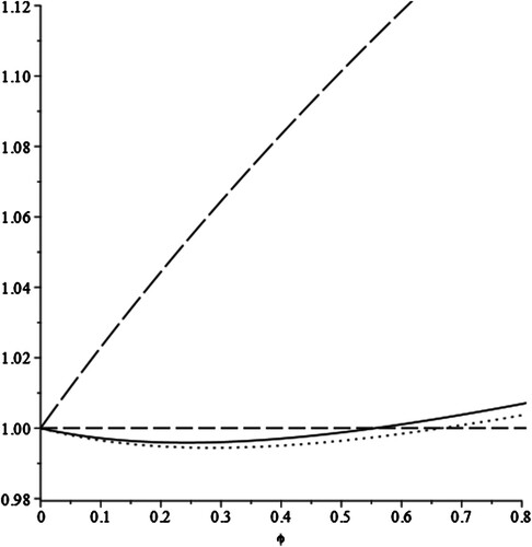
Figure 1 shows a graphical representation of the indirect utility ratio (27) as a function of trade freeness when smaller market size is the only source of country $H$’s locational disadvantage and market structure is perfectly competitive.⁶ With trade freeness measured along the horizontal axis, the two convex curves correspond to two indirect utility ratios evaluated for a smaller value of $\gamma$ (solid line style) and a larger value of $\gamma$ (dotted line style). The horizontal dashed line is the unit benchmark. When the indirect utility ratio is above (below) that line, country $H$ is better (worse) off with trade than in autarky. For ease of comparison, the upward sloping long-dashed curve reports the gains from trade. The figure shows an interesting pattern: as the country starts to liberalise trade from autarky, initially the pains from trade due to the contraction of the strategic industry dominate the gains from trade leading to lower indirect utility than in autarky. Only later on, as trade liberalisation proceeds, the situation is reversed with the gains dominating the pains from trade. By making the pains from trade more salient, a larger value of $\gamma$ increases the degree of trade freeness that has to be attained before the gains start to dominate the pains.

Figure 1. Indirect utility ratio and trade freeness (perfect competition without comparative advantage).

Read the detailed description of this figure

Graph with trade freeness on the horizontal axis and the indirect utility ratio on the vertical axis. There are three curves and a horizontal line. Two U-shaped curves correspond to two indirect utility ratios evaluated for a smaller value of γ (solid line style) and a larger value of γ (dotted line style). The horizontal dashed line is the unit benchmark. The third upward sloping long-dashed curve reports the gains from trade. The three curves and the horizontal line all originate from the same point on the vertical axis with value 1. Away from that point, the upward sloping long-dashed curve never crosses the horizontal dashed line. The two U shaped curves cut the horizontal line from below. This happens for a value of trade freeness that is smaller for the solid than for the dotted curve.

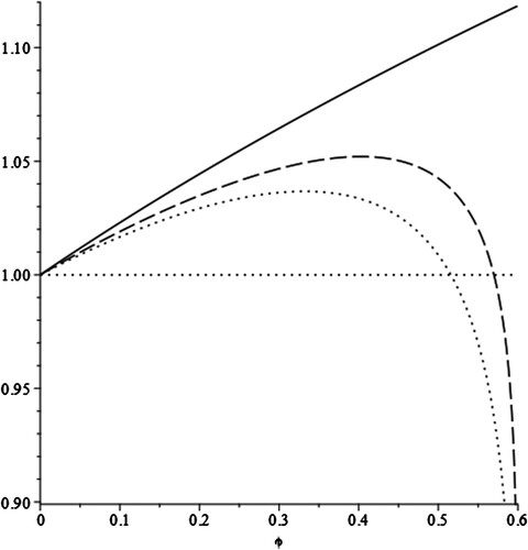
Figure 2 shows an analogous graphical representation of the indirect utility ratio (28) when market size market structure is monopolistically competitive.⁷ The two curves corresponding to the indirect utility ratios evaluated for smaller $\gamma$ (dashed line style) and larger $\gamma$ (dotted line style) are now concave. The horizontal dotted line is the unit benchmark while the upward sloping solid curve reports the gains from trade. The figure shows a different pattern than before: as the country starts to liberalise trade from autarky, initially the gains from trade dominate the pains from trade leading to higher indirect utility than in autarky. However, as trade liberalisation proceeds, the situation is reversed with the pains dominating the gains. The reason for this difference with respect to Figure 1 is that, as discussed above, under monopolistic competition structural transformation gains momentum as trade gets freer, whereas the oppositive happens under perfect competition. Moreover, as one would expect, a larger value of $\gamma$ decreases the degree of trade freeness that can be attained before the pains start to dominate the gains.

Figure 2. Indirect utility ratio and trade freeness (monopolistic competition without comparative advantage).

Read the detailed description of this figure

Graph with trade freeness on the horizontal axis and the indirect utility ratio on the vertical axis. There are three curves and a horizontal line. Two inverted U-shaped curves correspond to two indirect utility ratios evaluated for a smaller value of γ (dashed line style) and a larger value of γ (dotted line style). The horizontal dotted line is the unit benchmark. The third upward sloping solid curve reports the gains from trade. The three curves and the horizontal line all originate from the same point on the vertical axis with value 1. Away from that point, the upward sloping long-dashed curve never crosses the horizontal dashed line. The two inverted U-shaped curves cut the horizontal line from above. This happens for a value of trade freeness that is smaller for the dotted than for the dashed curve.

4.2. No market size difference

With $L_H=L_F$ expressions (25) and (26) simplify to (29) ${{\displaystyle \frac{W_H^{\mathrm{PC}}(\varphi )}{W_H^{\mathrm{PC}}(0)}}|}_{L_H/L_{F=1}}={\left[1+{\displaystyle \frac{\varphi }{(a+\varphi )(1+\mathrm{a\varphi })}(a^2-1)}\right]}^{\gamma }{\left(1+{\displaystyle \frac{\varphi }{a}}\right)}^{\frac{\alpha }{\epsilon }}$(29) and (30) ${{\displaystyle \frac{W_H^{\mathrm{MC}}(\varphi )}{W_H^{\mathrm{MC}}(0)}}|}_{L_H/L_{F=1}}={\left[1+{\displaystyle \frac{\varphi }{(a-\varphi )(1-\mathrm{a\varphi })}(a^2-1)}\right]}^{\gamma }{\left(1+\varphi {\displaystyle \frac{a-\varphi }{1-\mathrm{a\varphi }}}\right)}^{\frac{\alpha }{\epsilon }}$(30) respectively.

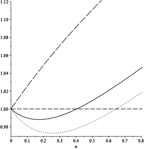
Figures 3 shows a graphical representation of the indirect utility ratio (29) as a function of trade freeness when comparative disadvantage is the only source of country $H$’s locational disadvantage and market structure is perfectly competitive.⁸ The figure exhibits the same qualitative features as Figure 1. As trade freeness starts to increase from autarky, the pains from trade initially dominate the gains from trade. Then, as trade liberalisation proceeds, the situation is reversed with the gains dominating the pains.

Figure 3. Indirect utility ratio and trade freeness (perfect competition without market size difference).

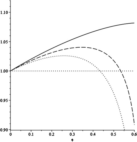
Analogously, Figure 4 shows a graphical representation of the indirect utility ratio (30) as a function of trade freeness when comparative disadvantage is the only source of country $H$’s locational disadvantage and market structure is monopolistically competitive.⁹ The figure exhibits the same qualitative features of Figure 2. As trade freeness starts to increase from autarky, the gains from trade initially dominate the pains from trade. Then, as trade liberalisation proceeds, the situation is reversed with the pains dominating the gains.

Figure 4. Indirect utility ratio and trade freeness (monopolistic competition without market size difference).

4.3. Role of scale elasticity

Beyond their graphical representations, expressions (25) and (26) can be used to further highlight the role of the scale elasticity $\gamma$ that regulates the strength of the positive nation-wide externality arising from employment in the strategic sector. In particular, they allow one to explicitly determine the threshold scale of elasticity above which the pains from trade dominate the gains from trade and below which the reverse holds.

Specifically, solving $W_H^{\mathrm{PC}}(\varphi )/W_H^{\mathrm{PC}}(0)=1$ and $W_H^{\mathrm{MC}}(\varphi )/W_H^{\mathrm{MC}}(0)=1$ for $\gamma$ determines the threshold scale elasticity as (31) ${\gamma }^{\mathrm{PC}}=-{\displaystyle \frac{\alpha }{\epsilon }{\displaystyle \frac{\ln \left(1+{\displaystyle \frac{\varphi }{a}}\right)}{\ln \left(1-{\displaystyle \frac{\varphi }{a+\varphi }{\displaystyle \frac{L_F}{L_H}\left[\left({\displaystyle \frac{L_H}{L_F}-1}\right)-{\displaystyle \frac{a^2-1}{1+\mathrm{a\varphi }}}\right]}}\right)}}}$(31) with perfect competition, and (32) ${\gamma }^{\mathrm{MC}}=-{\displaystyle \frac{\alpha }{\epsilon }{\displaystyle \frac{\ln \left(1+\varphi {\displaystyle \frac{a-\varphi }{1-\mathrm{a\varphi }}}\right)}{\ln \left(1+{\displaystyle \frac{\varphi }{1-\mathrm{a\varphi }}{\displaystyle \frac{L_F}{L_H}\left[a\left({\displaystyle \frac{L_H}{L_F}-1}\right)+{\displaystyle \frac{a^2-1}{a-\varphi }}\right]}}\right)}}}$(32) with monopolistic competition. For $\gamma ={\gamma }^{\mathrm{PC}}$ and $\gamma ={\gamma }^{\mathrm{MC}}$ gains and pains exactly offset each other so that country $H$ is indifferent between trade and autarky. The pains dominate the gains for $\gamma >{\gamma }^{\mathrm{PC}}$ and $\gamma >{\gamma }^{\mathrm{MC}}$, with the opposite happening for $\gamma <{\gamma }^{\mathrm{PC}}$ and $\gamma <{\gamma }^{\mathrm{MC}}$. With reference to the figures discussed in the previous section, ${\gamma }^{\mathrm{PC}}$ and ${\gamma }^{\mathrm{MC}}$ are the value of the scale elasticity corresponding to the intersections of the indirect utility ratios with the horizontal unit benchmark. Those figures show that, holding $\alpha /\epsilon$, $L_H/L_F$ and $a$ constant, the intersections depend on $\varphi$ as implied by (31) and (32).

Consider, now, the two polar cases. With no comparative advantage ($a=1$), for $B_H(\varphi )/B_H(0)<1$ to hold, country $H$ must be larger than country $F$ ($L_H>L_F$) with perfect competition, but smaller than country $F$ ($L_H<L_F$) with monopolistic competition. Expressions (31) and (32) evaluate to (33) ${\gamma }^{\mathrm{PC}}{|}_{a=1}=-{\displaystyle \frac{\alpha }{\epsilon }{\displaystyle \frac{\ln (1+\varphi )}{\ln \left(1-{\displaystyle \frac{\varphi }{1+\varphi }\left(1-{\displaystyle \frac{L_F}{L_H}}\right)}\right)}}}$(33) and (34) ${\gamma }^{\mathrm{MC}}{|}_{a=1}=-{\displaystyle \frac{\alpha }{\epsilon }{\displaystyle \frac{\ln (1+\varphi )}{\ln \left(1-{\displaystyle \frac{\varphi }{1-\varphi }\left({\displaystyle \frac{L_F}{L_H}-1}\right)}\right)}}}$(34) respectively. The fact that (33) is an increasing function of $\varphi$ implies that, as trade becomes freer, with perfect competition the scale elasticity required for the pains to dominate the gains rises. In other words, the range of values of $\gamma$ for which trade reduces indirect utility with respect to autarky becomes narrower when trade freeness increases. Therefore, when trade is already deeply liberalised, a given value of $\gamma$ is less likely to fall in the region where further trade deepening reduces the indirect utility ratio by downsizing the strategic industry. It is then harder to argue against trade based on a shrinking strategic industry when trade liberalization is deeper rather than shallower. In contrast, the fact that (34) is a decreasing function of $\varphi$ implies that, as trade becomes freer, with monopolistic competition the scale elasticity required for trade pains to dominate trade gains falls. The range of values for $\gamma$ for which trade reduces the indirect utility ratio is, therefore, wider for higher rather than lower trade freeness. It is then easier to argue against trade based on a shrinking strategic industry, for deeper rather than shallower trade liberalisation. Moreover, for given $\varphi$, with perfect (monopolistic) competition the larger is the market size difference between countries, the smaller (larger) is the scale elasticity required for the pains to dominate the gains.

With no market size difference ($L_H=L_F$), for $B_H(\varphi )/B_H(0)<1$ to hold, country $H$ must have a comparative disadvantage in the strategic industry ($a<1$). Expressions (31) and (32) then simplify to (35) ${\gamma }^{\mathrm{PC}}{|}_{L_H/L_{F=1}}=-{\displaystyle \frac{\alpha }{\epsilon }{\displaystyle \frac{\ln \left(1+{\displaystyle \frac{\varphi }{a}}\right)}{\ln \left(1-{\displaystyle \frac{\varphi }{a+\varphi }{\displaystyle \frac{1-a^2}{1+\mathrm{a\varphi }}}}\right)}}}$(35) and (36) ${\gamma }^{\mathrm{MC}}{|}_{L_H/L_{F=1}}=-{\displaystyle \frac{\alpha }{\epsilon }{\displaystyle \frac{\ln \left(1+\varphi {\displaystyle \frac{a-\varphi }{1-\mathrm{a\varphi }}}\right)}{\ln \left(1-{\displaystyle \frac{\varphi }{1-\mathrm{a\varphi }}{\displaystyle \frac{1-a^2}{a-\varphi }}}\right)}}}$(36) respectively. The former expression is an increasing function of $\varphi$ so that, as trade becomes freer, with perfect competition the scale elasticity required for the pains to dominate the gains also increases. The latter expression is a decreasing function of $\varphi$ and thus, as trade becomes freer, with monopolistic competition the scale elasticity required for the pains to dominate the gains decreases. As before, with perfect (monopolistic) competition it is harder (easier) to argue against trade based on a shrinking strategic industry for shallower (deeper) trade liberalisation. Moreover, for any given $\varphi$, with perfect (monopolistic) competition the stronger is the comparative disadvantage (smaller $a$) between countries, the smaller (larger) is the scale elasticity required for the pains to dominate the gains.

To summarise, no matter whether country $H$’s locational disadvantage arises from comparative advantage or market size difference, we can state:

Proposition 2 – Trade liberalization and national welfare. For a country with a locational disadvantage in the strategic industry, freer trade makes it more (less) difficult for the pains for trade to dominate the gains from trade under perfect (monopolistic) competition.

The reason for the asymmetry between perfect and imperfect competition arises from the fact that, as already discussed, under monopolistic competition firms in the strategic industry become more sensitive to comparative advantage and market size differences as trade is liberalised. As a result, structural change becomes more disruptive. The opposite holds under perfect competition.

5. CONCLUSION

We have modelled ‘strategic’ industries as exerting positive externalities on the national economy. We have argued that our understanding of the role of industrial policy in the presence of such industries may benefit from an extension of quantitative general equilibrium trade models making the extent and pattern of trade-induced reallocations more salient.

We have made those features relevant for national welfare by introducing the notion of the ‘social footprint’ of globalisation as the result of suboptimal, trade-induced, structural transformation in the presence of positive externalities from strategic industries.

For proof of concept, we have used simple workhorse versions of the most popular trade models featuring two countries and two industries, only one of which is ‘strategic’, to highlight the role of the elasticity of the externality to the scale of the strategic industry. We have also discussed the consequences of alternative assumptions on market structure, showing that how a market structure is modelled matters much more than generally understood in the literature on quantitative trade models.

The ‘scale elasticity’ of the strategic industry is a key parameter determining the unpriced costs and benefits of trade-induced structural change (and thus whether the country where the strategic industry shrinks gains at all from trade). Its value is not available off-the-shelf and how to estimate it is not straightforward and depends on the interpretation of the externality. Nonetheless, as highlighted by Colantone et al. (2022), in the case of technological spillovers a promising approach could be to find a way to extend the estimation strategy developed by Bartelme et al. (2019) for a closed-economy quantitative model from the structural estimation of intra-sectoral spillovers to that of inter-sectoral spillovers. This would provide the ingredients for computing the economy-wide scale elasticities of the different sectors and quantitatively assess their strategic relevance.

Hence, future developments of this line of research should focus on the structural estimation of intra- and inter-industry externalities to compute the nation-wide scale elasticities of the different industries and quantitatively assess their strategic relevance. Moreover, while for simplicity we have not considered the internal geography of countries, due attention should be paid to the spatial decay of those externalities as crucial determinants of the nation-wide scale elasticities.

ACKNOWLEDGEMENTS

We thank the editor and two anonymous reviewers for precious advice.

DISCLOSURE STATEMENT

No potential conflict of interest was reported by the author(s).

Additional information

Funding

This project has received funding from the European Research Council (ERC) under the European Union’s Horizon 2020 research and innovation programme (grant agreement number 789049-MIMAT-ERC-2017-ADG).

Notes

1 https://single-market-economy.ec.europa.eu/industry/strategy_en.

2 As discussed by Head and Mayer (2023), CES demand implies that substitution across products follows a simple share proportionality. In contrast, the demand systems typically used in industrial organisations allow for cross-elasticities that depend on a similarity in observable attributes. This is clearly more realistic but it is also more demanding in terms of data availability and computational challenges, especially when it comes to general equilibrium applications. Head and Mayer (2023) show that at the aggregate level the combination of CES and monopolistic competition can offer a useful approximation of the more complex demand systems and market structures found in the standard toolkit of industrial organisations.

3 Formally, $L_H^d>\alpha L_H$ holds if and only if $L_H/L_F<a(a+\varphi )/(1+\mathrm{a\varphi })$ is satisfied. Hence, even when country $H$ is larger ($L_H/L_F>1$), with trade it can still gain employment in the strategic industry if it has a strong enough comparative advantage ($a>1$). Vice versa, even when the country has a comparative disadvantage ($a<1$), with trade it can still gain employment in the strategic industry if it is smaller enough ($L_H/L_F<1$).

4 Formally, $L_H^d>\alpha L_H$ holds if and only if $L_H/L_F>(1-\mathrm{a\varphi })/[a(a-\varphi )]$ is satisfied. Hence, even when country $H$ is smaller ($L_H/L_F<1$), with trade it can still gain employment in the strategic industry if it has a strong enough comparative advantage ($a>1$). Vice versa, even when the country has a comparative disadvantage ($a<1$), with trade it can still gain employment in the strategic industry if it is larger enough ($L_H/L_F>1$).

5 Formally, with monopolistic competition $a<1$ is a sufficient condition for $d^2\mathrm{GF}{T}_H^{\mathrm{MC}}(\varphi )/d{\varphi }^2<0$, while $a>1$ is a necessary condition for $d^2\mathrm{GF}{T}_H^{\mathrm{MC}}(\varphi )/d{\varphi }^2>0$.

6 In Figure 1 the parameter values are $\alpha =0.5$, $\epsilon =2.1$, $a=1$, $L_H/L_F=1.5$, $\gamma =0.83$ (solid convex curve) or $\gamma$ $=0.85$ (dotted convex curve).

7 In Figure 2 the parameter values are $\alpha =0.5$, $\epsilon =2.1$, $a=1$, $L_H/L_F=0.6$, $\gamma =0.05$ (dashed concave curve) or $\gamma$ $=0.08$ (dotted concave curve).

8 In Figure 3 the parameter values are $\alpha =0.5$, $\epsilon =2.1$, $a=0.9$, $L_H/L_F=1$, $\gamma =2$ (solid convex curve) or $\gamma$ $=2.5$ (dotted convex curve).

9 In Figure 4 the parameter values are $\alpha =0.5$, $\epsilon =2.1$, $a=0.9$, $L_H/L_F=1.1$, $\gamma =0.1$ (dashed concave curve) or $\gamma$ $=0.2$ (dotted concave curve).

REFERENCES

- Arkolakis, C., Costinot, A., & Rodríguez-Clare, A. (2012). New trade models, same old gains? American Economic Review, 102(1), 94–130. https://doi.org/10.1257/aer.102.1.94
- Armington, P. S. (1969). A theory of demand for products distinguished by place of production. Staff Papers, 16(1), 159–178. https://doi.org/10.2307/3866403
- Bartelme, D., Costinot, A., Donaldson, D., & Rodríguez-Clare, A. (2019). The Textbook Case for Industrial Policy: Theory Meets Data. NBER WP 26193.
- Caliendo, L., Dvorkin, M., & Parro, F. (2019). Trade and labor market dynamics: General equilibrium analysis of the China trade shock. Econometrica, 87(3), 741–835. https://doi.org/10.3982/ECTA13758
- Caliendo, L., & Parro, F. (2015). Estimates of the trade and welfare effects of NAFTA. The Review of Economic Studies, 82(1), 1–44. https://doi.org/10.1093/restud/rdu035
- Caliendo, L., & Parro, F. (2022). Trade policy. In E. Helpman, G. Gopinath, & K. Rogoff (Eds.), Handbook of international economics (Vol. 5, pp. 219–295). International Trade and Investment.
- Colantone, I., Ottaviano, G., & Stanig, P. (2022). The backlash of globalization. In E. Helpman, G. Gopinath, & K. Rogoff (Eds.), Handbook of international economics (Vol. 5, pp. 405–477). Elsevier.
- Costinot, A., & Rodríguez-Clare, A. (2014). Trade theory with numbers: Quantifying the consequences of globalization. In E. Helpman, G. Gopinath, & K. Rogoff (Eds.), Handbook of international economics (Vol. 4, pp. 197–261). Elsevier.
- Dhingra, S., Huang, H., Ottaviano, G., Paulo Pessoa, J., Sampson, T., & Van Reenen, J. (2017). The costs and benefits of leaving the EU: Trade effects. Economic Policy, 32(92), 651–705. https://doi.org/10.1093/epolic/eix015
- Eaton, J., & Kortum, S. (2002). Technology, geography, and trade. Econometrica, 70(5), 1741–1779. https://doi.org/10.1111/1468-0262.00352
- Head, K., & Mayer, T. (2014). Gravity equations: Workhorse, toolkit, and cookbook. In E. Helpman, G. Gopinath, & K. Rogoff (Eds.), Handbook of international economics (pp. 131–195). Elsevier.
- Head, K., & Mayer, T. (2023). Poor substitutes? Counterfactual methods in IO and trade compared. Review of Economics and Statistics. https://doi.org/10.1162/rest_a_01369
- Krugman, P. (1980). Scale economies, product differentiation, and the pattern of trade. The American Economic Review, 70(5), 950–959.
- Melitz, M. J. (2003). The impact of trade on intra-industry reallocations and aggregate industry productivity. Econometrica, 71(6), 1695–1725. https://doi.org/10.1111/1468-0262.00467