Three-dimensional numerical simulations and proper orthogonal decomposition analysis of flow over different bottom-mounted ribs

ABSTRACT

Turbulent flow over bottom-mounted ribs is investigated using three-dimensional (3D) Spalart-Allmaras Delayed Detached-Eddy Simulations (SADDES). The ribs are subjected to a boundary layer flow with a thickness of δ/H=0.73 at Re=1∗106(Re=U∞H/ν), where U∞ is the free stream velocity, H is the rib height and ν is the fluid kinematic viscosity. Mesh and time step convergence studies are conducted to determine the grid and time step resolution. The numerical model is validated against the previous published experimental data and numerical results. The effects of different ribs geometries on drag and lift coefficients, the wake flow structures, and the dominant frequencies are discussed. Dominant flow features are investigated by carrying out Proper Orthogonal Decomposition (POD) and quadrant analysis of velocities and pressure in the wake flow.

KEYWORDS:

• Bottom-mounted ribs
• 3D turbulent flow
• SADDES
• proper orthogonal decomposition

1. Introduction

Bottom-mounted rib structures are widely used in many industries, such as subsea covers to protect pipelines, heat exchangers and gas turbines. These structures are often exposed to a high Reynolds number flow. It is of great significance to investigate the hydrodynamic forces on the structures. For example, subsea structures are commonly subjected to strong current and wave and should be kept on their installation positions. For design and optimisation with safe operation, it is necessary to obtain the drag and lift coefficients on the structures.

There are many experimental studies carried out to analyse the high Reynolds flow over surface-mounted structures over decades. Arie et al. (1975) studied the flow over wall-mounted rectangular cylinders subjected to turbulent boundary layer flow and concluded that the pressure coefficient on the structure surface is correlated with the thickness of the boundary layer. Fully developed turbulent channel flow around prismatic obstacles was investigated by Martinuzzi and Tropea (1993) and it was found that there is a nominally two-dimensional middle region in the wake about the plane of symmetry behind the structures with an aspect ratio larger than 6. Liu et al. (2008) studied the unsteady characteristics of the flow over a two-dimensional (2D) square rib and the flapping behaviour of the separation bubble behind the rib is analysed.

Numerical simulations have also been used to study the flow over wall-mounted structures. Utnes and Ren (1995) analysed the turbulent flow around a wall-mounted cube by using Reynolds-averaged Navier-Stokes (RANS) equations with the two-equation $k-ϵ$ turbulence model. The results were in good agreement with the experimental data reported by Castro and Robins (1997). Hwang et al. (1999) carried out 2D simulations of turbulent flow around ribs with varying length using RANS combined with the $k-ϵ$ model. It was found that the length of the recirculation region behind the rib is dependent on the rib width. The recirculation length decreases linearly with the increasing height-to-width ratio of the rib cross-section. Orellano and Wengle (2000) compared Large Eddy Simulation (LES) with Direct Numerical Simulation (DNS) for turbulent flow over a wall-mounted fence. LES was able to provide satisfying results compared with the reference data of DNS while using less than 5% of the computational requirement of DNS. Schmidt and Thiele (2002) conducted Detached Eddy Simulation (DES) of high Reynolds number flow over wall-mounted cubes and compared the results with those obtained by LES and RANS simulations. It was shown that DES was capable of capturing the unsteadiness of the wake flow behind the cubes. Frederich et al. (2008) compared DES and LES by carrying out numerical simulations of flow around a wall-mounted cylinder. DES and zonal DES of high Reynolds number flow around a bottom-mounted cube were performed by Haupt et al. (2011). It was found that DES can obtain better results than RANS compared with the experimental data reported by Hoxey et al. (2002). Tauqeer et al. (2017) carried out 2D RANS simulations of flow over wall-mounted square, triangular and semi-circular structures using $k-ϵ$ model. The results were in good agreement with the experimental data obtained by Liu et al. (2008). Also, the highest values of drag coefficient were obtained from the square structure and the highest lift coefficient was obtained from the semi-circular structure.

After performing the numerical simulations of the flow over the ribs, it is necessary to analyse the coherent structures behind the ribs in order to understand the dominant flow structures which will benefit the engineering design of the rib geometries. In the present study, a data-driven postprocessing technique called proper orthogonal decomposition (POD) is used to study the wake flow behind the ribs. It has been widely used to capture the temporal–spatial characteristics of large-scale coherent structures and build a low-dimensional representation of the turbulent flow fields using only a finite number of modes according to Podvin (2009) and Lehnasch et al. (2011). Subcritical flow around a square cylinder at different distances from the bottom-wall was investigated using experiments by Shi et al. (2010). Vortex shedding was found to be totally suppressed when the obstacle is located at distances lower than $0.4D$ to the wall. POD was used to analyse the flow structures in the wake region and low-order approximations of the flow were constructed using the two most energetic POD modes. Muld et al. (2012a) carried out POD analysis of the turbulent flow around a high-speed train and the method showed good capacity in extracting key coherent structures of the flow. He et al. (2016) carried out experimental analysis of the turbulent flow around a square rib under different gaps to the bottom-wall. POD analysis was performed to investigate the dominant coherent structures downstream the rib. The analysis of the first POD modes showed that they tend to appear in pairs indicating the downstream convective nature of the turbulent structures. A low-order approximation of the flow with the first four POD modes was built to represent the unsteadiness of the flow. The flow over a wall-mounted square cylinder was studied using experiments by Leite et al. (2018) and POD analysis was carried out to identify coherent structures in the wake region. It was concluded that the symmetrical and anti-symmetrical vortices in the cylinder wake flow can be captured by the first four POD modes. Amor et al. (2019) employed different decomposition techniques to analyse the flow over a bottom-mounted square cylinder and the relationship between the flow scales and different modes was discussed. Resolvent analysis was employed to investigate the turbulent flow over a square rib with different gap ratios between the obstacle and the wall by He et al. (2019). It was observed that the reconstruction of the flow field using the most five energetic resolvent modes is in good agreement with the POD modes. Ikhennicheu et al. (2019) studied the coherent flow structures downstream a bottom-mounted square cylinder at $Re=2.5\times {10}^5$ using experiments. POD analysis was used to identify the main coherent structures and study the trajectories of the large-scale vortices behind the cylinder. Mercier et al. (2020) carried out experiments and numerical simulations to analyse the coherent flow structures behind a bottom-mounted square cylinder. Large-scale Kelvin-Helmholtz (K-H) vortices were observed in the wake region and their frequencies were identified using wavelet decomposition.

The three-dimensional (3D) Spalart-Allmaras Delayed Detached-Eddy Simulations (SADDES) are carried out to investigate the flow over different bottom-mounted ribs at a high Reynolds number of $1\times {10}^6$ in the present study. To the authors’ knowledge, there are only few numerical studies that were carried out on the flow at such high Reynolds number. The effects of different bottom-mounted ribs (square, trapezoidal and rectangular) on the hydrodynamic quantities and the vortical structures in the wake region behind the ribs are discussed in detail. In addition, 2D POD analysis is employed to identify dominant coherent structures of the wake flow behind the ribs. Quadrant analysis is used to study the contribution of the dominant POD modes to the turbulence production in the wake flow. The paper is organised as follows: the mathematical formulation, numerical methods, computational overview, convergence studies and validation studies are presented in Section 2. The results and discussion are presented in Section 3. Lastly, the conclusion is given in Section 4.

2. Mathematical formulation, numerical method, computational overview, convergence and validation studies

2.1. Mathematical formulation

The filtered Navier-Stokes equations of incompressible and viscous fluid applied in DDES simulations can be written as: (1) $\frac{\mathrm{\partial }{u}_i}{\mathrm{\partial }{x}_i}=0$(1) (2) $\frac{\mathrm{\partial }{u}_i}{\mathrm{\partial }t}+\frac{\mathrm{\partial }{u}_i{u}_j}{\mathrm{\partial }{x}_j}=-\frac{\mathrm{\partial }p}{\mathrm{\partial }{x}_i}+\nu \frac{{\mathrm{\partial }}^2{u}_i}{\mathrm{\partial }{x}_j{x}_j}-\frac{\mathrm{\partial }{u}_i^{\mathrm{\prime }}{u}_j^{\mathrm{\prime }}}{\mathrm{\partial }{x}_j}$(2) where i,j = 1,2,3 represent the streamwise, cross-stream and spanwise directions, respectively. u₁, u₂, and u₃ (also denoted as u, v and w) are their corresponding resolved velocity components. The unresolved stresses $-〈u_i^{\mathrm{\prime }}{u}_j^{\mathrm{\prime }}〉$ can be defined as: (3) $-〈u_i^{\mathrm{\prime }}{u}_j^{\mathrm{\prime }}〉={\nu }_t\left(\frac{\mathrm{\partial }{u}_i}{\mathrm{\partial }{x}_j}+\frac{\mathrm{\partial }{u}_j}{\mathrm{\partial }{x}_i}\right)$(3)

The one equation Sparlat-Allmaras model solves the transport equation for the turbulent eddy viscosity (ν_t) which is described as: (4) ${\nu }_t=\tilde{\nu }{f}_{v1}{f}_{v1}=\frac{X^3}{X^3+C_{v1}^3}X=\frac{\tilde{\nu }}{{\nu }_t}$(4) where $\tilde{\nu }$ is the modified turbulence viscosity and the constant $C_{v1}=7.1$. DES is a hybrid approach where RANS method is applied in the near-wall region and LES is used far away from the wall. The distance to the wall (d̃) is given as: (5) $\tilde{d}=min\left(d,C_{DES}\mathrm{\Delta }\right)$(5) where the minimum distance from the nearest wall is represented as d and the constant C_DES= 0.65. The length scale associated with the local grid spacing is given as Δ: (6) $\mathrm{\Delta }=max\left({\mathrm{\Delta }}_x,{\mathrm{\Delta }}_y,{\mathrm{\Delta }}_z\right)$(6) where ${\mathrm{\Delta }}_x,{\mathrm{\Delta }}_y,{\mathrm{\Delta }}_z$ denote the dimension of the grid cell in the streamwise, cross-stream and spanwise directions, respectively.

An improved version of DES, SADDES, is used in the present study. It employs a modified DES limiter d̃ given in (5) in order to prevent grid-induced separation (Spalart et al. 2006): (7) $\tilde{d}=d-f_{d}max\left(0,d-C_{DES}\mathrm{\Delta }\right)$(7)

2.2. Numerical methods

The open source Computational Fluid Dynamics (CFD) code OpenFOAM v2.4 is used in the present study. The code is a customised C++ engine with noticeable application in CFD. Pressure-Implicit with Splitting of Operators (PISO) algorithm is used. The second order schemes for gradient and divergence are Gauss linear; for Laplacian and interpolation, Gauss linear corrected and linear schemes are employed, respectively. The time integration is conducted by using the second order Crank–Nicolson method.

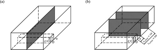
2.3. Computational overview

The computational domain used in this study is presented in Figure 1(a,b) and the height of the rib is denoted as H. Three different cross-section geometries are studied: square (with a bottom edge length of $B=H$), trapezoidal and rectangular. A bottom edge length of $B=4H$ is used for the trapezoidal and the rectangular ribs. The slope angle of the two sides of the trapezoidal rib is $\alpha ={45}^{\circ }$. The distance between the inlet and the centre of the rib bottom is $Lu=11.5H$ and the distance between the centre of the rib and the outlet is $Ld=40.5H$. The height of the computational domain is $Lh=20H$. According to Ong et al. (2010), a domain with $Lu=10H$, $Ld=20H$ and $Lh=10H$ is able to suppress the far-field effects on the structures. Therefore, the sizes of the XY domain in the present study can be considered sufficiently large. The spanwise length is $Lz=6H$, which is larger than that of $4H$ used in Prsic et al. (2019) and Tian et al. (2014).

Figure 1. Computational domain and boundary conditions: (a) 2D XY-plane and (b) 3D view.

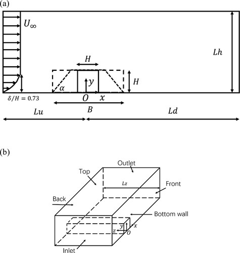
The boundary conditions are shown in Figure 1. The following boundary conditions are applied for all cases in this study:

•	At the inlet, a log profile for the fully developed boundary layer flow is used for the streamwise velocity, which is obtained by curve fitting of the experimental boundary layer profile reported by Arie et al. (1975). The vertical and spanwise velocities are set to zero. A boundary layer thickness of $\delta /H=0.73$ is employed, which is the same as that in the experiments carried out by Arie et al. (1975). A zero normal gradient is applied for the pressure at the inlet.
•	At the top boundary, the pressure and velocities are prescribed as zero normal gradient.
•	At the outlet, the velocities are prescribed as zero normal gradient and the pressure is set to be zero.
•	At the front and back boundary, periodic boundary conditions are used for all the quantities.
•	On the bottom wall and the surfaces of the structures, no-slip conditions are applied for the velocities and the pressure is set as zero normal gradient. The flow over the surfaces of the structures can be considered as fully developed turbulent. Therefore, a wall function based on the Spalding’s law of the wall (Spalding 1961) is used in the near-wall region.

2.4. Convergence studies

The mesh and time step convergence studies have been carried out. The results for each bottom-mounted rib are presented in Table 1. Two hydrodynamic quantities are analysed in this study: the time-averaged drag coefficient $\left(\overline{C_D}\right)$ in the streamwise direction and the time-averaged lift coefficient $\left(\overline{C_L}\right)$ in the cross-stream direction, which are given by: (8) $\overline{C_D}=\frac{\overline{F_X}}{{\displaystyle \frac{1}{2}\rho U_{\mathrm{\infty }}^2{A}_H}}\mathrm{a}\mathrm{n}\mathrm{d}\overline{C_L}=\frac{\overline{F_Y}}{{\displaystyle \frac{1}{2}\rho U_{\mathrm{\infty }}^2{A}_V}}$(8) where $\overline{F_X}$ is the time-averaged force acting on the rib surface in the streamwise direction while $\overline{F_Y}$ is the time-averaged force acting on the rib surface in the cross-stream direction, $\rho$ is the density of the fluid, $A_V$ is the vertical projected area and $A_H$ is the horizontal projected area of the ribs.

Table 1. Results for all the bottom-mounted ribs based on the mesh elements and the time-step.

Case		No. of cells	Grids in Z direction	Δt	$\overline{C_D}$	$\overline{C_L}$	Lw
	1	1,275,219	33	0.002	1.116	0.567	14.168
	2	1,652,970	33	0.002	1.121	0.572	13.626
Square rib	3	2,140,512	33	0.002	1.133	0.581	12.907
	4	2,140,512	33	0.001	1.132	0.580	12.907
	5	2,140,512	33	0.003	1.131	0.579	12.907
	6	3,113,472	48	0.002	1.133	0.581	13.172
	7	1,275,219	33	0.002	0.806	0.261	13.702
Trapezoidal rib	8	1,652,970	33	0.002	0.825	0.272	12.400
	9	2,140,512	33	0.002	0.844	0.287	10.195
	10	1,275,219	33	0.002	0.961	0.490	18.213
Rectangular rib	11	1,652,970	33	0.002	0.985	0.499	15.812
	12	2,140,512	33	0.002	1.006	0.527	11.755

For the XY-plane grid resolution study, three meshes with the same grid in the spanwise direction are used with an increment of 30% in the total number of elements between different cases for each rib: the square rib (Cases 1–3), the trapezoidal rib (Cases 7–9) and the rectangular rib (Cases 10–12). The results for $\overline{C_D}$ and $\overline{C_L}$ show good convergence for the square rib with relative differences around 1% between cases. Also, convergence for both trapezoidal and rectangular ribs has also been achieved, with the maximum relative differences of $\overline{C_D}$ being less than 3% and the maximum relative difference around 5% of $\overline{C_L}$ between cases. In addition, Cases 4 and 5 are simulated to show the dependence of the results on the time step resolution for the square cases with the same grid number as Case 3, which indicates that the relative differences of $\overline{C_D}$ and $\overline{C_L}$ are around 1% between cases. Finally, Case 6 is simulated with an increasing grid number in the spanwise direction and the relative differences are lower than 0.1% for $\overline{C_D}$ and $\overline{C_L}$, which shows that the grid number of 33 in the spanwise direction is enough. 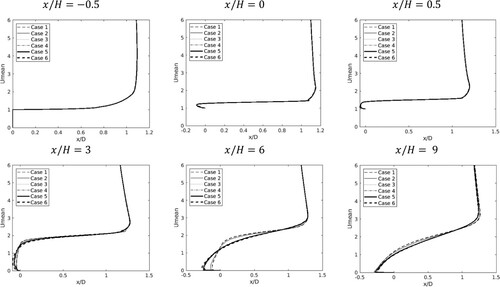Furthermore, the time- and spanwise-averaged streamwise velocity and pressure at $y/H=0.004$, which is close to the first layer above the bottom along the streamwise direction for the square rib (Cases 1–6), are shown in Figure 2. Both of the two profiles show good convergence between the different cases with similar recirculation lengths as shown in Figure 2(a). Likewise, a good agreement between Cases 1–6 for the pressure distribution is also displayed in Figure 2(b). The time- and spanwise-averaged streamwise velocity profiles in Figure 3 at different streamwise locations show that a good convergence has been achieved for Cases 1–6.

Figure 2. Profiles of the time- and spanwise-averaged (a) streamwise velocity and (b) pressure at $y/H=0.004$ for Cases 1–6.

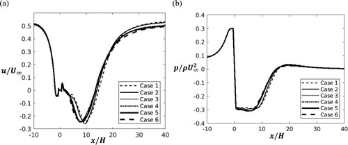
Figure 3. Time- and spanwise-averaged streamwise velocity profiles of Cases 1–6.

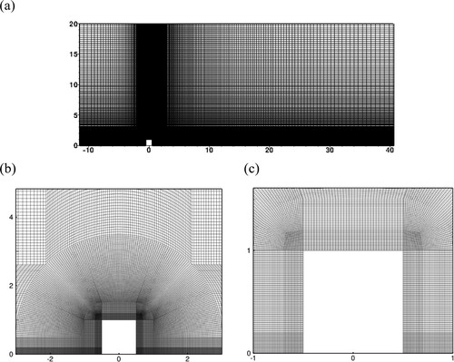
Therefore, based on these results, it can be concluded that a satisfactory grid and time step resolution have been achieved in Cases 3, 9 and 12 for the square rib, the trapezoidal rib and the rectangular rib, respectively and the results for the grid and the time step of these cases are analysed in the following sections. An example of the mesh is displayed in Figure 4 which shows the XY-plane of the converged Case 3.

Figure 4. Computational mesh of the square rib (Case 3): (a) full XY-plane domain and (b, c) closer view around the rib.

2.5. Validation studies

In order to validate the present SADDES numerical model at a high Reynolds number, the converged results of the flow over the square rib (Case 3) are compared with the experimental data reported by Liu et al. (2008). The time- and spanwise-averaged streamwise velocity profiles at different locations of the present results are compared with those of the experiments in Figure 5. It can be seen that the velocity profiles are overall in good agreement with the experimental data. The streamwise velocity profiles of the present numerical simulation display great similarity with the experimental data upstream and on the top of the square rib, while in the wake region behind the rib there are slight discrepancies between the present results and the experimental data. However, the negative parts of velocity profiles are well captured. The minor differences may be due to the difference of the Reynolds number between the experiment done by Liu et al. (2008) and the present numerical simulation. In addition, the recirculation zone behind the square rib of the present study is compared with the results reported by Liu et al. (2008). The recirculation zone is identified by using the wall-normal positions of the local maximum time- and spanwise-averaged root-mean-square value of streamwise velocity fluctuations as shown in Figure 6. It can be seen that the present predicted recirculation zone is almost the same as that obtained using experiments reported by Liu et al. (2008). Moreover, the drag coefficient and the recirculation length of Case 3 are compared with the published numerical results in Table 2. It can be seen that the present predicted values of $C_D$ and the recirculation length $L_w$ of the wake flow behind the square rib are in good agreement with those reported by Tauqeer et al. (2017).

Figure 5. Time-averaged streamwise velocities of Case 3 compared with the experimental data reported by Liu et al. (2008).

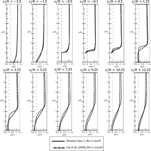
Figure 6. Wall-normal positions of the local maximum time- and spanwise-averaged root-mean-square value of the streamwise velocity fluctuations.

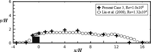
Table 2. Comparison of Case 3 with the numerical results reported by Tauqeer et al. (2017).

Configuration	Author	Flow conditions	$C_D$	$L_w$
Square	Case 3	$Re=1\times {10}^6$, $\delta /H=0.73$	1.133	12.907
	Tauqeer et al. (2017)	$Re=1\times {10}^6$, $\delta /H=0.73$	1.16	12.02

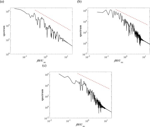
In addition, the spectra of the resolved streamwise velocity fluctuations obtained at $y/H=0.5$ with a distance of $0.5H$ to the back face of the three different ribs are shown in Figure 7. It is shown that the three spectra are observed to be close to the −5/3 slope in the inertial range, which indicates that the turbulence spectrum can be properly captured by the current simulations.

Figure 7. Power spectra of the velocity fluctuations at $y/H=0.5$ with a distance of $0.5H$ to the back face of the ribs for (a) square, (b) trapezoidal and (c) rectangular ribs. The red lines represent the −5/3 law. (This figure is available in colour online.)

3. Results and discussion

3.1. Hydrodynamic forces and flow field

The time histories of the hydrodynamic quantities $C_D$ and $C_L$ of the converged cases (Cases 3, 9 and 12) of the three ribs are shown in Figure 8 together with the phase-space plots of the two force coefficients. It can be seen that there exists unsteadiness in the time histories of the force coefficients which has also been reported in Tian et al. (2014) and Wu et al. (2020). The force coefficients of the trapezoidal rib show the weakest unsteadiness and the rectangular rib displays the strongest unsteadiness. 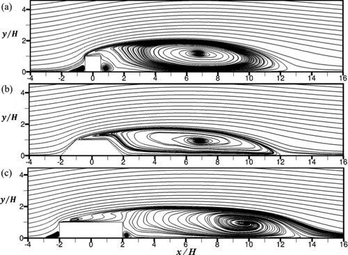Approximate linear correlations between the envelops of $C_D$ and $C_L$ are observed. The streamlines of the time- and spanwise-averaged flow are shown in Figure 9. For the three ribs, a large recirculation motion is observed behind the ribs. The recirculation motion is the longest for the square rib among the three ribs. For the square and rectangular ribs, there also exist two small recirculation motions in front of the ribs and in the corner of the back face of the ribs. The first one is caused by the downward flow to the bottom wall when the flow hits the front face of the rib, while the second one has similar behaviour when the flow hits the back face of the rib. Due to the inclination, the flow is more attached to the trapezoidal rib and the two small recirculation motions disappear.

Figure 8. Time histories of $C_D$, $C_L$ for (a) the square rib of Case 3; (c) the trapezoidal rib of Case 9 and (e) the rectangular rib of Case 12 and phase-space plots of $C_D$, $C_L$ for (b) the square rib; (d) the trapezoidal rib and (f) the rectangular rib.

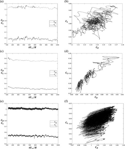
Figure 9. The streamlines of the time- and spanwise-averaged flows for (a) the square rib of Case 3; (b) the trapezoidal rib of Case 9; (c) the rectangular rib of Case 12.

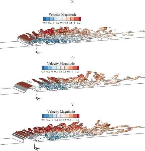
The three-dimensional instantaneous vortex structures identified by the $Q$ criterion proposed by Hunt et al. (1988) for the three ribs are shown at $t{U}_{\mathrm{\infty }}/H=1000$ in Figure 10. The $Q$ is given by: (9) $Q=\frac{1}{2}\left({\parallel \mathbf{\Omega }\parallel }^2-{\parallel \mathit{S}\parallel }^2\right)$(9) where $\mathit{S}$ is the rate of strain tensor and $\mathbf{\Omega }$ is the vorticity tensor. It can be seen that shear layers stem from the leading edges of the ribs where the flows separate and roll up in to small-scale streamwise vortices further downstream. It is observed that the complexity of the vortex structures is reduced for the rectangular and the trapezoidal ribs compared with the square rib. The vorticities behind the rectangular and the trapezoidal ribs are lower than that behind the square rib, which results in a reduced pressure difference between the front and back faces of the ribs and thus leads to lower drag coefficients for the two ribs than that of the square rib as shown in Figure 8. For the trapezoidal rib, as the flow is more attached to the rib surfaces, the small-scale vortex structures move further from the back face of the rib compared with the other ribs. For the rectangular rib, the shear layer on the top of the rib undergoes instability which may result in the strong unsteadiness of the hydrodynamic quantities as shown in Figure 8(e,f).

Figure 10. Instantaneous iso-surface of $Q=0.25$ at $t{U}_{\mathrm{\infty }}/H=1000$ for (a) the square rib of Case 3; (b) the trapezoidal rib of Case 9; (c) the rectangular rib of Case 12. (This figure is available in colour online.)

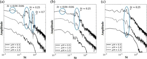
3.2. Spectral analysis

A Power Spectral Density (PSD) analysis is performed to obtain the dominant frequencies of the turbulent flow in the wake region. The cross-stream velocity signals are obtained at three streamwise positions and three heights at the middle of the spanwise direction ($z/H=3$). These points are at $L_x/H=0.5,3$ and 5.5 after the back face of the ribs and $y/H=0.5,1$ and 1.5. PSD of the cross-stream velocity signals is carried out by employing the Welch’s method (Welch 1967).

The frequency spectra of the cross-stream velocity for the three ribs are shown in Figures 11–13. For the square rib, a dominant frequency peak band is observed in Figure 11(a) centred at $St\approx 0.4$ close to the shear layer. This dominant frequency is associated with the Kelvin-Helmholtz (K-H) instability of the shear layer. This frequency value is close to that reported in Gu et al. (2017) ($St\approx 0.361$) and Gu et al. (2018) ($St\approx 0.42$) for the flow over bottom-mounted square ribs. At further downstream locations, as shown in Figure 11(b), the K-H instability becomes less obvious while another peak at $St\approx 0.2$ is observed. This frequency mode was also reported in Roos and Kegelman (1986) and Gu et al. (2018). According to their studies, the mode is related to vortex pairing in the separation bubble. For the trapezoidal rib as shown in Figure 12, a clear Strouhal number of $St\approx 0.3$ is observed close to the shear layer at $y/H=1.5$ for the three streamwise positions, which is associated with the K-H instability. The vortex pairing mode at $St\approx 0.15\sim 0.2$ is also shown at the three streamwise locations. According to Mercier et al. (2020), the energetic frequencies range between $St\approx 0.15$ and $St\approx 0.3$in the present study may indicate different patterns of K-H vortices emission with different time scales. For the rectangular rib as shown in Figure 13, the K-H instability mode is more obvious at a higher frequency of $St\approx 0.7$ compared with the other two ribs and the shear layer instability can be also observed in the vortical structures shown in Figure 10(c). The vortex pairing mode is observed at $St\approx 0.25$. Furthermore, there seems to be a low-frequency mode observed at $y/H=1.5$ for the three ribs. The low frequency is in the range of $St\approx 0.04\sim 0.06$. This low-frequency mode has been widely reported in Liu et al. (2008), Gu et al. (2018), Ikhennicheu et al. (2019) and Wu et al. (2020). According to Gu et al. (2018), this low frequency mode may be due to the flapping of the separation bubble.

Figure 11. Power spectra density of the cross-stream velocity ($v$) for the square rib at a distance of (a) $L_x/H=0.5$ (b) $L_x/H=3.5$ and (c) $L_x/H=5.5$ to the back face of the rib. (This figure is available in colour online.)

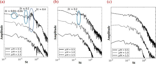
Figure 12. Power spectra density of the cross-stream velocity ($v$) for the trapezoidal rib at a distance of (a) $L_x/H=0.5$ (b) $L_x/H=3.5$ and (c) $L_x/H=5.5$ to the back face of the rib. (This figure is available in colour online.)

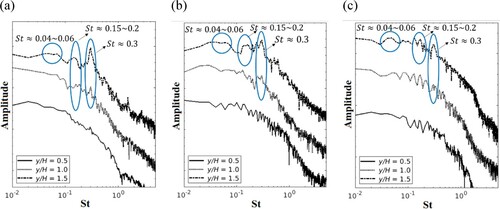
Figure 13. Power spectra density of the cross-stream velocity ($v$) for the rectangular rib at a distance of (a) $L_x/H=0.5$ (b) $L_x/H=3.5$ and (c) $L_x/H=5.5$ to the back face of the rib. (This figure is available in colour online.)

3.3. Proper orthogonal decomposition analysis

In order to analyse the complex flow structures behind the ribs, proper orthogonal decomposition is used to extract the energy containing structures in the wake region. This technique was proposed by Lumley (1967) to analyse the turbulent coherent structures. This method can also be applied to any scalar or vector quantities. In fluid mechanics, POD attempts to decompose a time-dependent flow variable $\mathit{q}\left(\mathit{\chi },t\right)$ (where $\mathit{\chi }$ denote the spatial coordinates and $t$ denotes the time, respectively) into a series of spatial modes ${\varphi }_{\mathit{j}}\left(\mathit{\chi }\right)$ and their corresponding temporal coefficients $a_j\left(t\right)$ as: (10) $\mathit{q}\left(\mathit{\chi },t\right)=\sum _j{a}_j\left(t\right){\varphi }_{\mathit{j}}\left(\mathit{\chi }\right)$(10) The POD modes ${\varphi }_{\mathit{j}}\left(\mathit{\chi }\right)$ are orthogonal satisfying ${\varphi }_{\mathit{i}}\left(\mathit{\chi }\right),{\varphi }_{\mathit{j}}\left(\mathit{\chi }\right)={\delta }_{ij}$ and can be obtained by eigenvalue decomposition of the spatial or temporal correlation matrix of the flow quantities as proposed by Lumley (1967), Sirovich (1987) and Meyer et al. (2007). As discussed in Taira et al. (2017), the modes can also be obtained by Singular Value Decomposition (SVD).

In the present study, POD analysis of the velocity components and the pressure at 2D planes shown in Figure 14 is carried out. The algorithm of the POD method is given as follows. The flow field data from the simulations is sampled and arranged in a matrix: (11) $\mathit{M}={\mathit{V}}_1^{\mathit{n}}=\left[{\mathit{v}}_1,{\mathit{v}}_2,\dots ,{\mathit{v}}_{\mathit{n}}\right]$(11) where ${\mathit{v}}_{\mathit{i}}$ ($i=1,2,3\dots n$) are column vectors containing the velocity components at each grid node in a 2D plane at the time step of $t_i\left(i=1,2,3\dots n\right)$ separated by the same time step $\mathrm{\Delta }{t}_{\mathrm{P}\mathrm{O}\mathrm{D}}$. The procedure is similarly applied for the pressure: (12) $\mathit{M}={\mathit{P}}_1^{\mathit{n}}=\left[{\mathit{p}}_1,{\mathit{p}}_2,\dots ,{\mathit{p}}_{\mathit{n}}\right]$(12)

Figure 14. Representation of the snapshots assembling along the (a) streamwise direction and the (b) spanwise direction.

The POD modes are obtained by applying SVD on the snapshot's matrix M: (13) $\mathit{M}=\mathit{U}\mathrm{\Sigma }{\mathit{V}}^{\mathit{T}}$(13) where U and V are the left and the right singular vectors of M, respectively. The column vectors of $\mathit{U}$are the POD modes ${\varphi }_{\mathit{j}}$ and the column vectors of $\mathit{V}$ denote the temporal coefficients $a_j\left(t\right)$ of the corresponding modes. They are both orthogonal matrices satisfying: (14) ${\mathit{V}}^{\mathit{T}}\mathit{V}=\mathit{I}$(14) (15) ${\mathit{U}}^{\mathit{T}}\mathit{U}=\mathit{I}$(15)

The diagonal matrix $\mathrm{\Sigma }=diag\left({\lambda }_1,{\lambda }_2,{\lambda }_3\dots {\lambda }_{\mathit{n}}\right)$ contains the singular values of the matrix $\mathit{M}$ and each diagonal value represents the energy carried by each POD mode. They are ordered as: (16) ${\lambda }_1>{\lambda }_2>{\lambda }_3>\dots >{\lambda }_{\mathit{n}}>0$(16)

In the present study, an economy-size SVD is performed by using the corresponding internal function in MATLAB, which means that for the rectangular matrix ${\mathit{M}}_{m\times n}$ with $m>n$, only the first $n$ columns of the left singular vectors are calculated and $\mathrm{\Sigma }$ is a $n\times n$ matrix.

3.3.1. Proper orthogonal decomposition analysis along the streamwise direction

In this section, POD analysis is made on a XY-plane in the middle of the spanwise direction at $z=3H$. The total number of spatial points of each snapshot is $m=129728$. According to Yang et al. (2017), the results obtained from POD analysis should be independent on the number of snapshots and the time step $\mathrm{\Delta }{t}_{\mathrm{P}\mathrm{O}\mathrm{D}}$ between the sampling flow fields snapshots. Therefore, a convergence study has to be done in order to determine the appropriate number of snapshots and the time step ($\mathrm{\Delta }{t}_{\mathrm{P}\mathrm{O}\mathrm{D}}$).

Due to the orthogonality of the POD modes, Muld et al. (2012a) proposed a method of the convergence study based on the orthogonality of the POD modes. If the scalar product between the leading POD modes defined as ${ϵ}_{ortho}=〈{\varphi }_{j,1},{\varphi }_{j,2}〉$ (1,2 denote different snapshots samples with different snapshots numbers and $j$ denotes the number of the modes) obtained using different numbers of snapshots equals 1, the POD modes have been fully converged. A similar test can also be conducted based on different time steps $\mathrm{\Delta }{t}_{\mathrm{P}\mathrm{O}\mathrm{D}}$ between snapshots. Figures 15 and 16 show the mean value of ${ϵ}_{ortho}$ of the ten most energetic velocities and pressure modes of all geometries. The value of ${ϵ}_{ortho}$ is obtained by comparing the POD modes based on different numbers of snapshots with the POD modes obtained based on the snapshots with the number of 800, which is used as the reference set of modes. This procedure is the same as done in Muld et al. (2012a, 2012b). A similar convergence test is done by calculating ${ϵ}_{ortho}$ comparing the POD modes based on different number of snapshots $S_{n\mathrm{P}\mathrm{O}\mathrm{D}}$ and time step $\mathrm{\Delta }{t}_{\mathrm{P}\mathrm{O}\mathrm{D}}$. The results given in Figures 15 and 16(a) are based on a reference snapshot of $S_{n\mathrm{P}\mathrm{O}\mathrm{D}}=800$with equal sampling time. The results shown in Figures 15 and 16(b) are based on a reference time step of $\mathrm{\Delta }{t}_{\mathrm{P}\mathrm{O}\mathrm{D}}=0.5H/U_{\mathrm{\infty }}$ and sampling time of $800H/U_{\mathrm{\infty }}$_. It can be seen that an acceptable convergence can be achieved when the number of snapshots is higher than 600 and $\mathrm{\Delta }{t}_{\mathrm{P}\mathrm{O}\mathrm{D}}$ is lower than $1H/U_{\mathrm{\infty }}$. A similar behaviour of the value ${ϵ}_{ortho}$ is also reported in Muld et al. (2012a, 2012b). Thus, the POD analyses of the present study are carried out using 1600 snapshots with $\mathrm{\Delta }{t}_{\mathrm{P}\mathrm{O}\mathrm{D}}=0.5H/U_{\mathrm{\infty }}$.

Figure 15. The mean value of ${ϵ}_{ortho}$ of the ten most energetic modes between different sets of snapshots of the velocity modes based on: (a) number of snapshots; (b) $\mathrm{\Delta }{t}_{\mathrm{P}\mathrm{O}\mathrm{D}}$ of the velocity modes.

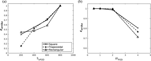
Figure 16. The mean value of ${ϵ}_{ortho}$ of the ten most energetic modes between different sets of snapshots of the pressure modes based on: (a) number of snapshots; (b) $\mathrm{\Delta }{t}_{\mathrm{P}\mathrm{O}\mathrm{D}}$ of the velocity modes.

3.3.1.1. The square rib

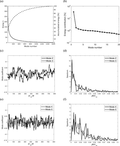
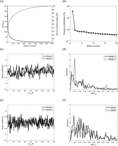
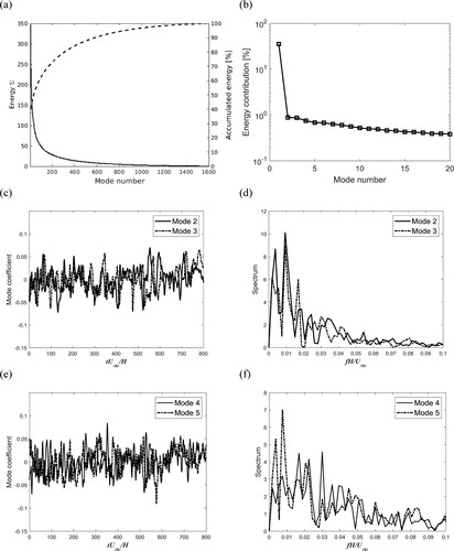
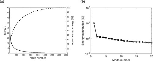
The energy distribution of all the velocity POD modes of the square rib is shown in Figure 17(a). It shows an exponential decay of the energy from the lower modes to the higher modes. The energy contribution of the first 20 POD modes is presented in Figure 17(b). The first POD mode corresponds to the mean flow containing almost 30% of the total energy of the velocity field in the 2D plane, while the following modes contribute less than 1% to the total energy. Figure 17(c,e) shows the temporal coefficients of Modes 2, 3 and Modes 4, 5. For Modes 2 and 3, a wave-like periodic behaviour is observed and the frequency spectrum of their temporal coefficients given in Figure 17(d) show similar peaks within the low frequency range. This indicates a large-scale travelling wave structure as reported in Semeraro et al. (2012) and Yang et al. (2017). The frequency spectra of mode temporal coefficients of Modes 4 and 5 are displayed in Figure 17(f) and a wide spectra distribution is observed, indicating a chaotic behaviour of Modes 4 and 5.

Figure 17. Modal decomposition of the velocities for the square rib: (a) energy of modes; (b) energy contribution of the 20 leading energetic modes; (c) temporal coefficients of Modes 2 and 3 and (d) frequency spectra of Modes 2 and 3; (e) temporal coefficients of Modes 4 and 5 and (f) frequency spectra of Modes 4 and 5.

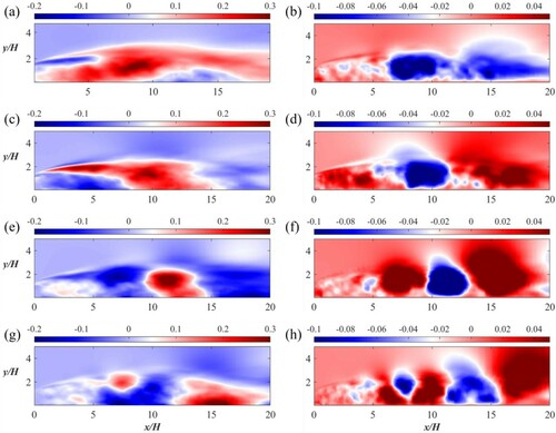
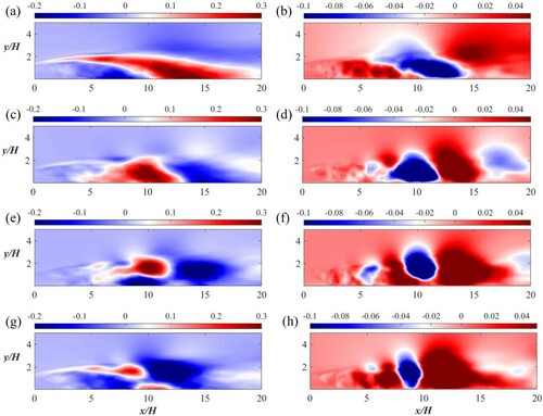
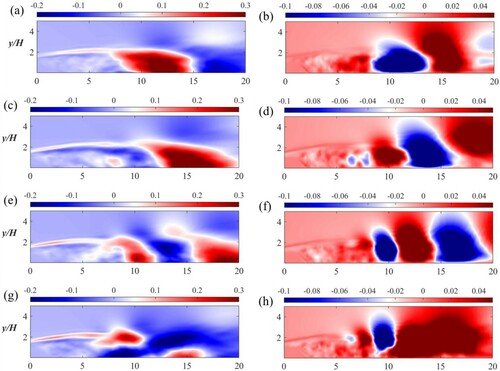
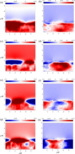
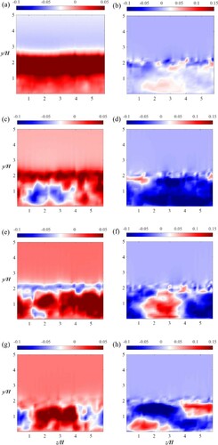
Contours of the POD velocity modes of the square rib are shown in Figure 18: (a) and (c) show the most energetic pair of the fluctuation modes (Modes 2 and 3), while (e) and (g) show the following pair (Modes 4 and 5) of the streamwise velocity. The pairs have similar level of energy as shown in Figure 17(b) indicating the downstream convection of the modes. The first pair of POD modes shows a strong shear layer around the edge of the wake flow, while the second pair shows positive and negative velocity regions with a shorter streamwise length scale compared with the first pair. Figure 18(b, d, f, h) displays the cross-stream velocity contours of Modes 2, 3 and Modes 4, 5. The positive and negative pairs are clearly seen and shorter length scale regions are also observed in the higher modes of Modes 4, 5 compared with those of Modes 2, 3.

Figure 18. POD modes of the streamwise (a, c, e, g) and cross-stream (b, d, f, h) velocities for the square rib: (a, b) POD Mode 2; (c, d) POD Mode 3; (e, f) POD Mode 4 and (g, h) POD Mode 5. (This figure is available in colour online.)

Figure 19(a) shows the $L_2$-norm distribution of all pressure POD modes for the square rib. The $L_2$-norm decays exponentially from the first modes to the following modes faster than the energy contained in the velocity modes as shown in Figure 17(a). The contribution of the most energetic modes is given in Figure 19(b). The first POD mode corresponds to the mean pressure and contains almost 35% of the total energy while the following fluctuation POD modes are much less energetic, with less than 2% of the total energy of the pressure field. The time histories of the coefficients of Modes 2 and 3 are shown in Figure 19(c) with the frequency spectra of the two modes in Figure 19(d). Different spectra of the two modes are shown, which indicates that the two modes cannot form a mode pair. A broadband distribution of the spectra is also observed within the low frequency range.

Figure 19. Modal decomposition of the pressure for the square rib: (a) energy of modes, (b) energy contribution of 20 most energetic modes (c) coefficients of Modes 2 and 3 and (d) frequency spectra of Modes 2 and 3.

Figure 20 displays the pressure contours of Modes 2–9 for the square rib which are fluctuation modes and contain 9.5% of the total energy of the pressure field in the 2D plane. Figure 20(a) shows a single large-scale pressure structure of Mode 2. Figure 20(b,c) shows the energetic pair of Modes 3 and 4, which display wave-packet form of structures with similar length scale of the structures and indicate downstream convection of the structures. Furthermore, the POD modes shown in Figure 20(d–g) also appear in pairs with a decreasing length scale of the turbulent structures that are mostly located on the shear layer behind the rib.

Figure 20. POD modes of the pressure for the square rib: (a) to (h) show POD Modes 2–9. (This figure is available in colour online.)

3.3.1.2. The trapezoidal rib

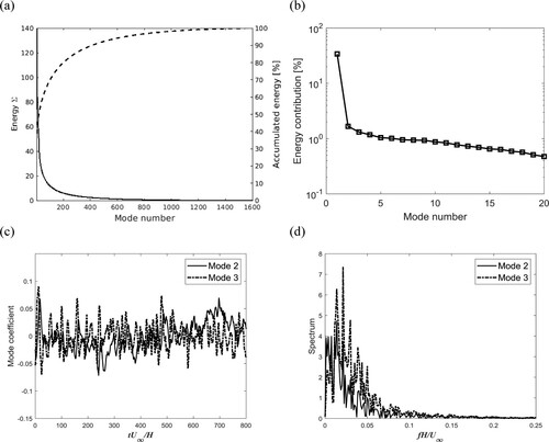
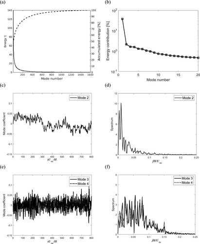
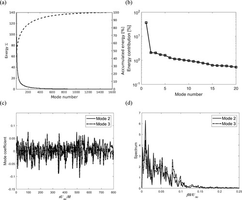
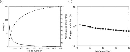
Figure 21(a) shows the energy distribution of the velocity POD modes for the trapezoidal rib case. An exponential decay of the energy from the first modes to the following higher modes is observed. Figure 21(b) displays the energy contribution of the 20 most energetic modes. The first mode corresponds to the mean flow and contributes with 35% of the total kinetic energy, while each of the following fluctuation modes contains less than 1% of the total energy. It can be seen that the mean flow occupies more energy than that of the square rib which also indicates that velocity fluctuations of wake flow behind the trapezoidal rib are weaker than those behind the square rib. The temporal coefficients as well as their frequency spectra of Modes 2 and 3 are shown in Figure 21(c,d). The peaks of the two Modes temporal coefficients are in the low frequency range and there is slight difference between the two modes. A chaotic behaviour is seen in the time histories of the coefficients of Modes 4 and 5 as shown in Figure 21(e) and the spectra of the two modes shown in Figure 21(f) display similar broadband distribution.

Figure 21. Modal decomposition of the velocities for the trapezoidal rib: (a) energy of modes; (b) energy contribution of most energetic modes; (c) coefficients of Modes 2 and 3 and (d) frequency spectra of Modes 2 and 3; (e) temporal coefficients of Modes 4 and 5 and (f) frequency spectra of Modes 4 and 5.

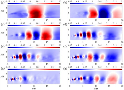
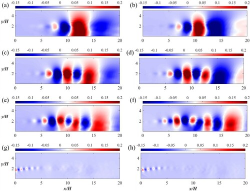
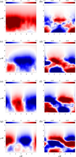
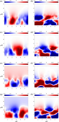
The most energetic modes are shown in Figure 22(a–h). There is also difference of the mode shapes between Modes 2 and 3, indicating that the two modes cannot form a pair. The streamwise velocities of the first mode show strong flow structures along the shear layer of the wake region. The second mode displays large-scale positive and negative alternate structures. The mode shapes of Modes 4 and 5 are similar, which can form a pair of modes. This pair of modes shows shorter vortical structures compared with the first pair located with a distance of $8\sim 10H$ from the back face of the rib. Together with the streamwise velocity modes, the large-scale spanwise rollers are indicated by these POD modes.

Figure 22. POD modes of the streamwise (a, c, e, g) and cross-stream (b, d, f, h) velocities for the trapezoidal rib: (a, b) POD Mode 2; (c, d) POD Mode 3; (e, f) POD Mode 4 and (g, h) POD Mode 5. (This figure is available in colour online.)

The $L_2$-norm distribution of the pressure modes for the trapezoidal rib is given in Figure 23(a). A faster exponential decay of the $L_2$-norm from the most energetic modes to the less energetic higher modes is observed compared with the velocity POD modes of the rib as shown in Figure 21(a). The energy contribution of the first 20 modes is presented in Figure 23(b). The first mode corresponds to the mean pressure, containing more than 35% of the total energy, while the higher modes contribute less than 2% of the total pressure energy. The temporal coefficient and the frequency spectrum of Mode 2 are shown in Figure 23(c,d). Low frequencies of the mode are observed. POD Modes 3 and 4 appear in pair which is indicated by their similar broadband frequency distribution of the temporal coefficients.

Figure 23. Modal decomposition of the pressure for the trapezoidal rib: (a) energy of modes; (b) energy contribution of the leading energetic modes; (c) coefficients of Mode 2; (d) frequency spectrum of Mode 2; (e) coefficients of Modes 3 and 4; (f) frequency spectra of Modes 3 and 4.

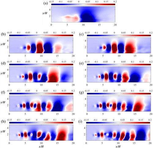
Figure 24 shows the pressure POD Modes 2–10 for the trapezoidal rib. They contain 10% of the total pressure energy in the 2D plane. The single Mode 2 is presented in Figure 24(a), and Figure 24(b,c) shows the most energetic pair of modes (Modes 3 and 4). The wave-packets are also shown, and their length scales are decreasing with higher modes. The high order POD modes are shown in Figure 24(d–i) and they are mostly located around the shear layer of the wake flow. Furthermore, the attachment of the fluctuations to the bottom wall is observed in these high order modes.

Figure 24. POD modes of the pressure for the trapezoidal rib: (a) to (i) show POD Modes 2–10. (This figure is available in colour online.)

3.3.1.3. The rectangular rib

Figure 25(a) shows the energy distribution of the velocity POD modes for the rectangular rib. It also has an exponential decay from lower order modes to higher order modes. Figure 25(b) shows the energy containing in the first 20 modes. The mean flow represented by the first mode contributes with 35% of the total kinetic energy, while the fluctuation modes have less than 1% of the total energy. The temporal coefficients of Modes 2 and 3 are given in Figure 25(c,d), which show the low frequency of the two modes. However, compared with those of the square and trapezoidal ribs, wider frequency distributions are observed for the two modes, indicating a more chaotic behaviour. Figure 25(e,f) displays the temporal information of the following pair of Modes 4 and 5. It is shown that the corresponding frequency spectra of this pair have wide distribution within the low frequency range.

Figure 25. Modal decomposition of the velocities for the rectangular rib: (a) energy of modes; (b) energy contribution of most energetic modes; (c) coefficients of Modes 2 and 3, and (d) frequency spectra of Modes 2 and 3; (e) coefficients of Modes 4 and 5, and (f) frequency spectra of Modes 4 and 5.

The most energetic pair of modes of the velocities in the streamwise plane (Modes 2 and 3) is shown in Figure 26(a–d) while the following pair (Modes 5 and 6) is given in Figure 26(e–h). The large-scale structures of the first pair are located far from the rib around $x/H=10\sim 15$. The streamwise and the cross-stream velocities of the first pair shows similar large-scale rollers structures convected downstream. Their streamwise length-scales are smaller than the first pair of modes of the square and trapezoidal ribs. The second pair displays shorter length scale compared with the first pair.

Figure 26. POD modes of the streamwise (a, c, e, g) and cross-stream (b, d, f, h) velocities for the rectangular rib: (a, b) POD Mode 2; (c, d) POD Mode 3; (e, f) POD Mode 4 and (g, h) POD Mode 5. (This figure is available in colour online.)

The $L_2$-norm distribution of all the pressure POD modes for the rectangular rib is shown in Figure 27(a). It has a faster exponential decay of the energy compared to the energy distribution of the velocity POD modes. The $L_2$-norm contribution of the most energetic modes is presented in Figure 27(b). The first mode corresponds to the mean pressure, contributing with 37% of the total energy, while each of the following modes contributes less than 2% of the total energy. Figure 27(c) shows the temporal coefficients of the pair of Modes 2 and 3 which show a chaotic behaviour. The frequency spectra of the first pair of modes is displayed in Figure 27(d) and they are more distributed in high frequency range compared to the other ribs.

Figure 27. Modal decomposition of the pressure for the rectangular rib: (a) energy of modes; (b) energy contribution of most energetic modes; (c) coefficients of Modes 2 and 3 and (d) frequency spectra of Modes 2 and 3.

The first four pairs of the fluctuation pressure POD modes for the rectangular rib are shown in Figure 28. In total, they have 13% of the pressure energy in the 2D plane. Figure 28(a,b) shows the first pair of modes (Modes 2 and 3) with a length scale close to the height of the large recirculation motion. The next two pairs of POD modes are shown in Figure 28(c–f) (Modes 4–7). They have higher streamwise wavenumber and are located on the edge of the shear layer. Also, small-scale turbulent structures can be seen in Figure 28(g,h), Modes 8 and 10, on the shear layer close to the rib.

Figure 28. POD modes of the pressure for the rectangular rib: (a) to (h) show POD Modes 2–9. (This figure is available in colour online.)

3.3.2. Quadrant analysis of velocity POD modes along the streamwise direction

A quadrant analysis of the most energetic fluctuation POD modes of streamwise and the cross-stream velocities in the XY-plane is performed to obtain detailed information of the contributions of fluid motions to the turbulence production in the wake flow. If $u>0$ and $v>0$, these events are found to be in the first quadrant and correspond to the outward motion of fluid (Q1 motion). If $u<0$ and $v>0$, they are located in the second quadrant and correspond to the ejection motion of the fluid (Q2 motion). If $u<0$ and $v<0$, they are in the third quadrant and are correlated to the inward motion of the fluid (Q3 motion). Finally, if $u>0$ and $v<0$, they are found to be in the fourth quadrant, and they correspond to sweeps of the fluid (Q4 motion).

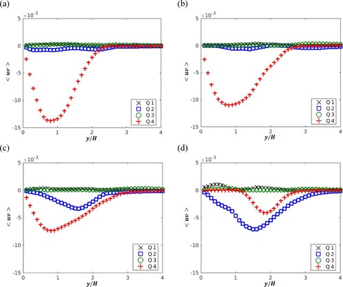
Figures 29–31 show the Reynolds shear stress of four quadrant plots of the first four POD fluctuation modes of all the ribs. The Reynolds shear stress is averaged in the streamwise direction in the wake region. It can be seen that for all analysed POD modes, there is a significant dominance of the gradient-type motions (Q2 and Q4) to the Reynolds shear stress over the counter-gradient-type motions (Q1 and Q3). These behaviours were also reported in Wallace et al. (1972) and Cai et al. (2009) in turbulent channel flows. Modes 2 and 3 mainly capture Q4 events which represents the sweep of high-momentum fluid towards the bottom wall. These sweep motions are mainly located around $1<y/H<2$ for the square rib while located around $y/H<1$ below the shear layer for the trapezoidal and rectangular ribs. Modes 4 and 5 tend to show dominant Q2 and Q4 events which represents the ejection of low-momentum fluid and the sweep of high-momentum fluid towards the bottom wall, respectively. They are mainly located around $1<y/H<2$ for all ribs. Furthermore, for the square rib, the contributions of the Q2 and Q4 events to the Reynolds shear stress are low in Mode 5, however, for the trapezoidal and rectangular ribs, their contributions are still strong.

Figure 29. Reynolds stress of four quadrant plots of the POD modes: (a) Mode 2, (b) Mode 3, (c) Mode 4 and (d) Mode 5 for the square rib. (This figure is available in colour online.)

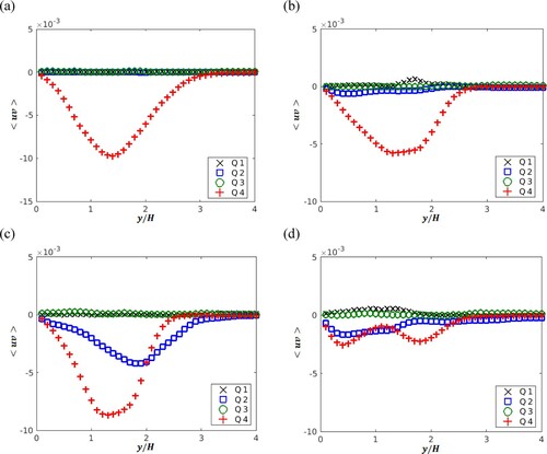
Figure 30. Reynolds stress of four quadrant plots of the POD modes: (a) Mode 2, (b) Mode 3, (c) Mode 4 and (d) Mode 5 for the trapezoidal rib. (This figure is available in colour online.)

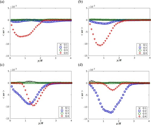
Figure 31. Reynolds stress of four quadrant plots of the POD modes: (a) Mode 2, (b) Mode 3, (c) Mode 4 and (d) Mode 5 for the rectangular rib. (This figure is available in colour online.)

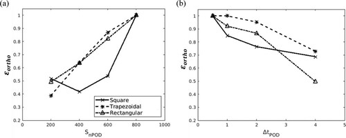
3.3.3. Proper orthogonal decomposition analysis on ZY planes

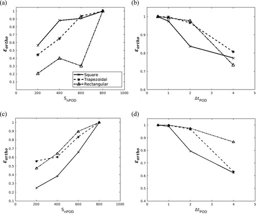
To further investigate the 3D characteristics of the coherent structures in the wake flows, POD analysis can also be applied to velocity components $\left(v,w\right)$ on ZY planes. Two planes are chosen with distances of $L_{x,\mathrm{P}\mathrm{O}\mathrm{D}}=1H$ and $6H$ to the back face of the ribs, as shown in Figure 14. The total number of the spatial points of each snapshot ranges from 12,342–15,972 depending on the rib shapes and meshes on the planes. A convergence study of the most energetic modes is done in order to determine an acceptable number of snapshots and time step. Figure 32 shows the mean value of ${ϵ}_{ortho}$ of the ten most energetic POD modes of all geometries between different numbers of snapshots and the time step. It can be seen that an acceptable convergence can be achieved when $\mathrm{\Delta }{t}_{\mathrm{P}\mathrm{O}\mathrm{D}}$ is 0.5 and a total of 1600 snapshots are used to conduct the analysis for each bottom-mounted rib.

Figure 32. The mean value of ${ϵ}_{ortho}$ of the ten most energetic modes between different sets of snapshots of the velocity modes based on: (a) number of snapshots; (b) $\mathrm{\Delta }{t}_{\mathrm{P}\mathrm{O}\mathrm{D}}$ of the velocity modes at $L_{x,\mathrm{P}\mathrm{O}\mathrm{D}}=1H$ behind the ribs; (c) number of snapshots; (d) $\mathrm{\Delta }{t}_{\mathrm{P}\mathrm{O}\mathrm{D}}$ of the velocity modes at $L_{x,\mathrm{P}\mathrm{O}\mathrm{D}}=6H$ behind the ribs.

3.3.3.1. The square rib

The energy distribution of all the velocity POD modes with $L_{x,\mathrm{P}\mathrm{O}\mathrm{D}}=1H$ is shown in Figure 33(a), while the energy contribution of the 20 leading modes is presented in detail in Figure 33(b). The first mode also corresponds to the mean flow, contributing with more than 9% of the total energy, while the following modes contribute with less than 2% of the kinetic energy of the flow in the 2D plane.

Figure 33. Modal decomposition of the velocities at $L_{x,POD}=1H$: (a) energy of modes; (b) energy contribution of most energetic modes; (c) coefficients of Modes 2 and 3 and (d) frequency spectra of Modes 2 and 3.

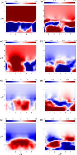
Contours of the POD velocity modes with $L_{x,POD}=1H$ are shown in Figure 34: (a) and (c) show the first pair of the fluctuation modes (Modes 2 and 3), while (e) and (g) show the second pair (Modes 4 and 5) of the cross-stream velocity. The two modes of each pair have similar level of energy as shown in Figure 33(b) indicating the downstream convection of the flow modes. Both pairs show a strong shear layer above the rib height which is located on the edge of the wake flow. Figure 34(b, d, f, h) displays the spanwise velocity contours of Modes 2, 3 and Modes 4, 5, showing more complex turbulent structures which indicates a chaotic flow in the spanwise direction inside the near wake region.

Figure 34. POD modes of the velocities at $L_{x,POD}=1H$ after the square rib: (a, b) POD Mode 2; (c, d) POD Mode 3; (e, f) POD Mode 4; and (g, h) POD Mode 5 with the cross-stream velocities (a, c, e, g) and the spanwise velocities (b, d, f, h). (This figure is available in colour online.)

The energy distribution of the velocity POD modes at $L_{x,\mathrm{P}\mathrm{O}\mathrm{D}}=6H$ behind the square rib is shown in Figure 35(a). An exponential decay of the energy distribution with the mode number is observed and the energy contribution of the most energetic modes is presented in Figure 35(b). It can be seen that only fluctuation modes appear since the mean values for $v,w$ are small at this streamwise location.

Figure 35. Modal decomposition of the velocities at $L_{x,POD}=6H$: (a) energy of modes, (b) energy contribution of most energetic modes.

Contours of the POD velocity modes with $L_{x,POD}=6H$ downstream the square rib are shown in Figure 36 and all of them can be considered fluctuation modes. For the first pair of Modes 1 and 2, the structures occupy the whole area of the wake region. Large-scale positive and negative regions of the cross-stream velocity indicate strong downwards and upwards flows. Together with the spanwise velocity as shown in Figure 36(b,d), Modes 1 and 2 represent large-scale streamwise vortices. Modes 3 and 4 of the second pair have smaller length-scale comparing with Modes 1 and 2. The modes shapes also represent streamwise vortices with a smaller spanwise length.

Figure 36. POD modes of the velocities at $L_{x,\mathrm{P}\mathrm{O}\mathrm{D}}=6H$ after the square rib: (a, b) POD Mode 1; (c, d) POD Mode 2; (e, f) POD Mode 3; and (g, h) POD Mode 4 with the cross-stream velocities (a, c, e, g) and the spanwise velocities (b, d, f, h). (This figure is available in colour online.)

3.3.3.2. The trapezoidal rib

The energy distribution of the velocity modes at $L_{x,\mathrm{P}\mathrm{O}\mathrm{D}}=1H$ downstream the trapezoidal rib is given in Figure 37(a), showing the exponential decay of energy from lower modes to higher modes. The energy contribution of the first 20 modes is presented in Figure 37(b). The first mode, corresponding to the mean flow, contains 8% of the total energy, while each of the high order POD modes contribute with less than 2% of the energy. Contours of the POD velocity modes at $L_{x,\mathrm{P}\mathrm{O}\mathrm{D}}=1H$ behind the trapezoidal rib are shown in Figure 38. Figure 38(a–d) shows two most energetic single fluctuation modes (Modes 2 and 3), while (e) to (h) show the pair of Modes 4 and 5. The complex and chaotic flow behaviours are shown in these modes. Figure 39(a) shows the energy distribution of all the velocity POD modes at $L_{x,\mathrm{P}\mathrm{O}\mathrm{D}}=6H$ behind the trapezoidal rib with a lower exponential decay compared with that at $L_{x,\mathrm{P}\mathrm{O}\mathrm{D}}=1H$. However, different from that of the square rib, the energy fraction of the first mode given in Figure 39(b) is around 2% of the total energy of the two components in the 2D plane and it still can represent the mean flow. Figure 40(a–h) gives the first two pairs of the cross-stream and spanwise velocities of POD modes (Modes 2, 3 and Modes 4, 5) at $L_{x,\mathrm{P}\mathrm{O}\mathrm{D}}=6H$ downstream the trapezoidal rib with structures distributed throughout the centre part of the wake region. The first pair clearly shows large-scale streamwise vortical structures with low spanwise wavenumber while the second pair also displays strong streamwise vortical structures with relatively higher spanwise wavenumber.

Figure 37. Modal decomposition of the velocities at $L_{x,POD}=1H$ after the trapezoidal rib: (a) energy of modes; (b) energy contribution of most energetic modes.

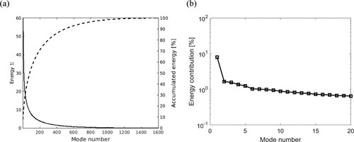
Figure 38. POD modes of the velocities at $L_{x,POD}=1H$ after the trapezoidal rib: (a, b) POD Mode 2; (c, d) POD Mode 3; (e, f) POD Mode 4; and (g, h) POD Mode 5 with the cross-stream velocities (a, c, e, g) and the spanwise velocities (b, d, f, h). (This figure is available in colour online.)

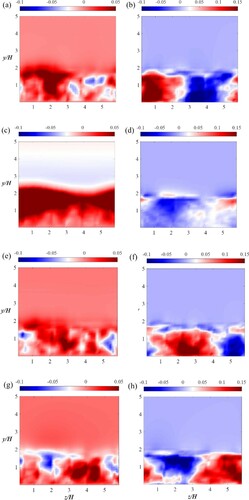
Figure 39. Modal decomposition of the velocities at $L_{x,POD}=6H$ after the trapezoidal rib: (a) energy of modes; (b) energy contribution of most energetic modes.

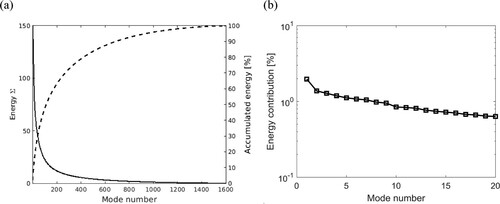
Figure 40. POD modes of the velocities at $L_{x,POD}=6H$ after the trapezoidal rib: (a, b) POD Mode 2; (c, d) POD Mode 3; (e, f) POD Mode 4; and (g, h) POD Mode 5 with the cross-stream velocities (a, c, e, g) and the spanwise velocities (b, d, f, h). (This figure is available in colour online.)

3.3.3.3. The rectangular rib

Figure 41(a) shows the energy distribution of all velocity POD modes at $L_{x,\mathrm{P}\mathrm{O}\mathrm{D}}=1H$ after the back face of the rectangular rib with an exponential decay. The energy contribution of the first 20 modes is shown in detail in Figure 41(b) with the first mode dominating the flow with 9% of the total energy in the 2D plane, while each of the following fluctuation modes contain less than 2% of the energy contribution. POD velocity modes at $L_{x,POD}=1H$ after the rectangular rib are shown in Figure 42 and give complex flow structures: (a) to (d) show the fluctuation Modes 2 and 3 with strong structures around the shear layer at $y/H\sim 2$ with a few vortical structures inside the near wake region. This pair of modes does not seem to have significant large-scale turbulent structures inside the wake region. Modes 4 and 5 are displayed in Figure 42(e–h) showing a large-scale cross-stream length vortical structure centred at the rib height.

Figure 41. Modal decomposition of the velocities at $L_{x,POD}=1H$ after the rectangular rib: (a) energy of modes; (b) energy contribution of most energetic modes.

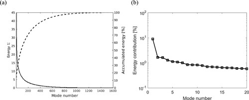
Figure 42. POD modes of the velocities at $L_{x,POD}=1H$ behind the rectangular rib: (a, b) POD Mode 2; (c, d) POD Mode 3; (e, f) POD Mode 4; and (g, h) POD Mode 5 with the cross-stream velocities (a, c, e, g) and the spanwise velocities (b, d, f, h). (This figure is available in colour online.)

The energy distribution of all velocity POD modes at $L_{x,POD}=6H$ after the back face of the rectangular rib is given in Figure 43(a). The energy contribution of the first 20 modes is shown in Figure 43(b) with the most energetic mode contributing with only 2.5% of the kinetic energy, however, it can be considered a representation of the mean flow. The following modes contain less than 2% of energy contribution individually. Contours of the POD velocity modes at $L_{x,POD}=6H$ downstream the rectangular rib are shown in Figure 44: (a,b) show the single mode of the fluctuation Modes 2. The cross-stream velocity of Mode 2 represents spanwise uniform downward flow in the wake and the spanwise velocity of this mode represents the flow towards the two spanwise directions. The following pair of Modes 3 and 4 is shown in Figure 44(c,d) and (e,f) representing streamwise vorticities. Figure 44(g,h) displays Mode 5 which represents an ejection motion in the wake flow.

Figure 43. Modal decomposition of the velocities at $L_{x,POD}=6H$ after the rectangular rib: (a) energy of modes, (b) energy contribution of most energetic modes.

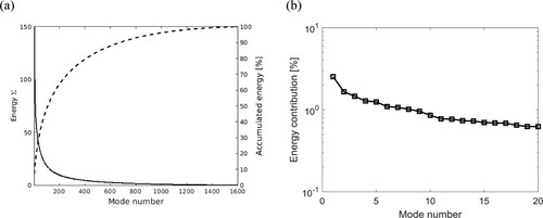
Figure 44. Modal decomposition of the velocities at $L_{x,POD}=6H$ after the rectangular rib: (a, b) POD Mode 2; (c, d) POD Mode 3; (e, f) POD Mode 4; and (g, h) POD Mode 5 with the cross-stream velocities (a, c, e, g) and the spanwise velocities (b, d, f, h). (This figure is available in colour online.)

4. Conclusion

In the present study, Spalart-Allmaras Delayed Detached-eddy simulations of flows over three different bottom-mounted ribs subjected to a boundary layer with a thickness of $\delta /H=0.73$ at $Re=1.0\times {10}^6$ are carried out. Convergence studies based on the time- and spanwise-averaged hydrodynamic quantities $\overline{C_D}$ and $\overline{C_L}$ are performed to determine the grid and time step resolutions. The time- and spanwise-averaged streamwise velocities behind the square rib and the location of the maximum time- and spanwise-averaged streamwise velocity fluctuations were compared with the experimental data reported by Liu et al. (2008) and a generally good agreement is achieved. The present predicted $C_D$ and the recirculation length $L_w$ behind the square rib are in good agreement with the numerical results reported by Tauqeer et al. (2017). Results of the hydrodynamic quantities and the turbulent wake flow were analysed. 2D proper orthogonal decomposition of the velocities and the pressure is used to extract the most energetic modes and careful convergence studies have been carried out to determine the total number of snapshots and the time step between the snapshots. The main conclusions can be outlined as follows:

1. The complexity of the vortical structures is reduced for the rectangular and the trapezoidal ribs compared with the square rib, resulting in reduced pressure differences of the rectangular and trapezoidal ribs and thus lower drag coefficients compared with the square rib.

2. A positive correlation between the time-histories of $C_D$ and $C_L$ for the three structures is observed. The streamlines of the time- and spanwise-averaged flows for the three ribs display large recirculation motions behind the ribs. The square rib produces the longest recirculation motion among the three ribs. There are two small recirculation motions in front of the ribs and in the corner of the back face of the ribs for the square and rectangular ribs while for the trapezoidal rib, the flow streamlines are attached to the rib surface with no other small recirculation motion.

3. A spectral analysis employing the Welch’s method is carried out. For the square rib, a dominant frequency peak is observed at $St\approx 0.4$, which is associated with the K-H instability of the shear layer. Another peak at $St\approx 0.2$ is observed and it is related to the vortex pairing in the separation bubble. A clear Strouhal number of $St\approx 0.3$ is obtained for the trapezoidal rib, which is associated with the K-H instability. For the rectangular rib, the K-H instability mode is obvious at a frequency of $St\approx 0.7$ and the vortex pairing mode is observed at $St\approx 0.25$. In addition, a low-frequency mode of $St\approx 0.04\sim 0.06$ is observed at $y/H=1.5$ for the three ribs, which may correspond to the flapping of the separation bubble.

4. The energy contained in the POD modes show an exponential decay from the first modes to the higher modes. For the flow velocity components and pressure at the 2D XY plane, the first mode corresponding to the mean flow contains more than 30% of the total energy. Most of the POD modes of the velocities and pressure fluctuation display in pairs indicating the downstream convection of the flow structures. The first pair of fluctuation POD modes shows strong shear layer stemming from the rib. High order fluctuation modes on this XY plane display a wave-packet form of structures with alternate positive and negative value regions and their length scales decrease with the increasing order. The structures of the high order pressure modes are mainly located around the shear layer of the wake flow.

5. Quadrant analysis of the most energetic fluctuation POD modes of streamwise and the cross-stream velocities in the XY-plane shows a significant dominance of the gradient-type motions (Q2 and Q4) to the Reynolds shear stress over the counter-gradient-type motions (Q1 and Q3) for all ribs. Moreover, the two most energetic fluctuation modes mainly capture Q4 events located below the shear layer and the following two modes show dominant Q2 and Q4 events.

6. The POD modes of the cross-stream and spanwise velocities at the two YZ planes are analysed. With a distance of $1H$ to the ribs back face, the POD modes are mainly located around the shear layer. For the square rib, with a distance of $6H$ to the rib back face, due to the small mean value of the cross-stream velocity and the zero mean spanwise velocity, there is no POD mode for the mean flow and the POD modes of the velocities represent streamwise vorticities with different length-scales. For the trapezoidal and rectangular ribs, the first mode corresponds to the mean flow and the fluctuation modes also display streamwise vortices. These streamwise vortical structures indicate the strong motions in the spanwise direction.

Acknowledgements

This study was supported with computational resources provided by the Norwegian Metacenter for Computational Science (NOTUR), under Project No: NN9372K.

Disclosure statement

No potential conflict of interest was reported by the author(s).

Additional information

Funding

This study was supported with computational resources provided by the Norwegian Metacenter for Computational Science (NOTUR) [Project No: NN9372K].

References

- Amor C, Pérez JM, Schlatter P, Vinuesa R, Le Clainche S. 2019. Soft computing techniques to analyze the turbulent wake of a wall-mounted square cylinder. In: International Workshop on Soft Computing Models in Industrial and Environmental Applications. Cham: Springer; p. 577–586.
- Arie M, Kiya M, Tamura H, Kanayama Y. 1975. Flow over rectangular cylinders immersed in a turbulent boundary layer (part 1. Correlation between pressure drag and boundary-layer characteristics). BullJSME. 18:1260–1268.
- Cai WH, Li FC, Zhang HN, Li XB, Yu B, Wei JJ, Hishida K. 2009. Study on the characteristics of turbulent drag-reducing channel flow by particle image velocimetry combining with proper orthogonal decomposition analysis. Phys Fluids. 21(11):115103.
- Castro IP, Robins AG. 1977. The flow around a surface-mounted cube in uniform and turbulent streams. J Fluid Mech. 79(2):307–335.
- Frederich O, Wassen E, Thiele F. 2008. Prediction of the flow around a short wall-mounted finite cylinder using LES and DES1. JNAIAM. 3(3–4):231–247.
- Gu H, Liu M, Li X, Huang H, Wu Y, Sun F. 2018. The effect of a low-frequency structure on passive scalar transport in the flow over a surface-mounted, rib. Flow Turbul Combust. 101(3):719–740.
- Gu H, Yang J, Liu M. 2017. Study on the instability in separating-reattaching flow over a surface-mounted rib. Int J Comut Fluid Dyn. 31(2):109–121.
- Haupt SE, Zajaczkowski FJ, Peltier LJ. 2011. Detached eddy simulation of atmospheric flow about a surface mounted cube at high Reynolds number. J Fluids Eng. 133(3):1–8.
- He C, Liu Y, Gan L, Lesshafft L. 2019. Data assimilation and resolvent analysis of turbulent flow behind a wall-proximity rib. Phys Fluids. 31(2):025118.
- He C, Liu Y, Peng D, Yavuzkurt S. 2016. Measurement of flow structures and heat transfer behind a wall-proximity square rib using TSP, PIV and split-fiber film. Exp Fluids. 57(11):165.
- Hoxey RP, Richards PJ, Short JL. 2002. A 6 m cube in an atmospheric boundary layer flow-part 1. Full-scale and wind-tunnel results. Wind Struct. 5(2–4):165–176.
- Hunt JC, Wray AA, Moin P. 1988. Eddies, streams, and convergence zones in turbulent flows.
- Hwang RR, Chow YC, Chiang TP. 1999. Numerical predictions of turbulent flow over a surface-mounted rib. J Eng Mech. 125(5):497–503.
- Ikhennicheu M, Germain G, Druault P, Gaurier B. 2019. Experimental study of coherent flow structures past a wall-mounted square cylinder. Ocean Eng. 182:137–146.
- Lehnasch G, Jouanguy J, Laval JP, Delville J. 2011. POD based reduced-order model for prescribing turbulent near wall unsteady boundary condition. In: Stanislas M, Jimenez J, Marusic I, editors. Progress in wall turbulence: understanding and modeling. ERCOFTAC Series, Vol. 14. Dordrecht: Springer; p. 301–308. doi:https://doi.org/10.1007/978-90-481-9603-6_31.
- Leite HF, Avelar AC, Abreu LD, Schuch D, Cavalieri A. 2018. Proper orthogonal decomposition and spectral analysis of a wall-mounted square cylinder wake. J Aerosp Technol Manag. 10:1–15. doi:https://doi.org/10.5028/jatm.v10.867.
- Liu YZ, Ke F, Sung HJ. 2008. Unsteady separated and reattaching turbulent flow over a two-dimensional square rib. J Fluids Struct. 24(3):366–381.
- Lumley JL. 1967. The structure of inhomogeneous turbulent flows. Atmospheric turbulence and radio wave propagation.
- Martinuzzi R, Tropea C. 1993. The flow around surface-mounted, prismatic obstacles placed in a fully developed channel flow (data bank contribution).
- Mercier P, Ikhennicheu M, Guillou S, Germain G, Poizot E, Grondeau M, Druault P. 2020. The merging of Kelvin–Helmholtz vortices into large coherent flow structures in a high Reynolds number flow past a wall-mounted square cylinder. Ocean Eng. 204:107274.
- Meyer KE, Pedersen JM, Özcan O. 2007. A turbulent jet in crossflow analysed with proper orthogonal decomposition. J Fluid Mech. 583:199–227.
- Muld TW, Efraimsson G, Henningson DS. 2012a. Mode decomposition on surface-mounted cube. Flow Turbul Combust. 88(3):279–310.
- Muld TW, Efraimsson G, Henningson DS. 2012b. Flow structures around a high-speed train extracted using proper orthogonal decomposition and dynamic mode decomposition. Comput Fluids. 57:87–97.
- Ong MC, Utnes T, Holmedal LE, Myrhaug D, Pettersen B. 2010. Numerical simulation of flow around a circular cylinder close to a flat seabed at high Reynolds numbers using a k–ϵ model. Coastal Eng. 57(10):931–947.
- Orellano A, Wengle H. 2000. Numerical simulation (DNS and LES) of manipulated turbulent boundary layer flow over a surface-mounted fence. Eur J Mech-B/Fluids. 19(5):765–788.
- Podvin B. 2009. A proper-orthogonal-decomposition-based model for the wall layer of a turbulent channel flow. Phys Fluids. 21(1):015111.
- Prsic MA, Ong MC, Pettersen B, Myrhaug D. 2019. Large Eddy simulations of flow around tandem circular cylinders in the vicinity of a plane wall. J Mar Sci Technol. 24(2):338–358.
- Roos FW, Kegelman JT. 1986. Control of coherent structures in reattaching laminar and turbulent shear layers. AIAA J. 24(12):1956–1963.
- Schmidt S, Thiele F. 2002. Comparison of numerical methods applied to the flow over wall-mounted cubes. Int J Heat Fluid Flow. 23(3):330–339.
- Semeraro O, Bellani G, Lundell F. 2012. Analysis of time-resolved PIV measurements of a confined turbulent jet using POD and Koopman modes. Exp Fluids. 53(5):1203–1220.
- Shi LL, Liu YZ, Wan JJ. 2010. Influence of wall proximity on characteristics of wake behind a square cylinder: PIV measurements and POD analysis. Exp Therm Fluid Sci. 34(1):28–36.
- Sirovich L. 1987. Turbulence and the dynamics of coherent structures. I. Coherent structures. Q Appl Math. 45(3):561–571.
- Spalart PR, Deck S, Shur ML, Squires KD, Strelets MK, Travin A. 2006. A new version of detached-eddy simulation, resistant to ambiguous grid densities. Theor Comput Fluid Dyn. 20(3):181.
- Spalding DB. 1961. A single formula for the law of the wall. J Appl Mech. 28(3):455–458.
- Taira K, Brunton SL, Dawson ST, Rowley CW, Colonius T, McKeon BJ, Ukeiley LS. 2017. Modal analysis of fluid flows: An overview. AIAA J. 55:4013–4041.
- Tauqeer MA, Li Z, Ong MC. 2017. Numerical simulation of flow around different wall-mounted structures. Ships Offsh Struct. 12(8):1109–1116.
- Tian X, Ong MC, Yang J, Myrhaug D. 2014. Large-eddy simulation of the flow normal to a flat plate including corner effects at a high Reynolds number. J Fluids Struct. 49:149–169.
- Utnes T, Ren G. 1995. Numerical prediction of turbulent flow around a three-dimensional surface-mounted obstacle. Appl Math Model. 19(1):7–12.
- Wallace JM, Eckelmann H, Brodkey RS. 1972. The wall region in turbulent shear flow. J Fluid Mech. 54(1):39–48.
- Welch P. 1967. The use of fast Fourier transform for the estimation of power spectra: a method based on time averaging over short, modified periodograms. IEEE Trans Audio Electroacoust. 15(2):70–73.
- Wu W, Meneveau C, Mittal R. 2020. Spatio-temporal dynamics of turbulent separation bubbles. J Fluid Mech. 883:A45-1–A45-37.
- Yang J, Liu M, Wu G, Gu H, Yao M. 2017. On the unsteady wake dynamics behind a circular disk using fully 3D proper orthogonal decomposition. Fluid Dyn Res. 49(1):015510.