Operability analysis of traditional small fishing boats in Indonesia with different loading conditions

ABSTRACT

Many ship accidents are experienced by small boats. With a large number of small fishing boats in Indonesia, the risk of potential ship accidents is high. Therefore, an operability analysis must be conducted for various loading conditions to address any safety issues due to severe vessel motion. The net cargo of a fishing boat will change during its operation at sea and then will affect the vessel’s seakeeping characteristics. This study aims to determine the effect of changes in load and their effect on a traditional fishing boat’s operability in Indonesia, considering the ship’s intact stability. In addition, this study also highlights the response of the ship roll motion to prevent stability failure. The stability curve is used to relate ship stability analysis to seakeeping analysis. Percentage operability and Operability Robustness Index are used to assess the root mean square (RMS) roll response and the ship's expected maximum roll motion.

KEYWORDS:

• Fishing boat
• ship stability
• percentage operability
• Operability Robustness Index (ORI)
• seakeeping

1. Introduction

Indonesia is an archipelagic country consisting of 17,504 islands whose coastline length is 108,000 km. The exclusive economic area of Indonesia is about 6,400,000 km² which is 3.37 times larger than the country’s land area and contributes to the local population’s welfare and sustenance. Fishing is a critically important industry for Indonesia.

The Ministry of Maritime and Fisheries Affairs Republic of Indonesia allocates fishing boats to Indonesian fishers. From 2010–2014 the Ministry allocated 1000 of 30 Gross Tonnage (GT) fishing boats to local fishers, while in 2016, 3500 fishing boats with sizes varying between 5 and 30 GT made of fibreglass were allocated. This policy aims to increase Indonesia's food security from the maritime sector (Bappenas 2010). Based on Statistics Indonesia (2019), the total number of fishing vessels in Indonesia from 2000–2016 was 543,845 (with and without an engine).

However, according to Food and Agriculture Organization (FAO) (2000), fishing at sea is a risky activity with the highest mortality rate due to accidents. FAO (2000) gave examples of the mortality rate in several countries by comparing it with the national average, which was up to 30 times larger in the US and 21 times larger in Italy. In Australia, the rate was 143 per 100,000 compared to the national average of 8.1 per 100.000.

In Table 1, the types of fishing vessel accidents are presented by Wang et al. (2005) and Ugurlu et al. (2020). The table shows the total number and percentage of each fishing vessel’s accident type. Some researchers studied a particular accident, such as Davis et al. (2019), who investigated the primary cause of capsizing accidents for fishing vessels. Obeng et al. (2022a) investigated the risk influencing factors for capsizing of the small fishing trawler boat which considered the different operational scenarios using Object-Oriented Bayesian Network (OOBN). From their study, the human factor in terms of training and experience was identified as the most critical influencing factor. Domeh et al. (2021) investigated the risk analysis for the man overboard (MOB) using OOBN. The results of the study can provide important safety-based information for small fishing vessel operations.

Table 1. The accident types for fishing vessels.

References	Accident Types	Total	Percentage
(Ugurlu et al. 2020)	Collision	56	27.05
	Sinking	55	26.57
	Occupational Accident	39	18.84
	Grounding	26	12.56
	Man Overboard	26	12.56
	Fire-Explosion	2	0.97
	Others	3	1.45
(Wang et al. 2005)	Machinery damage	233	62.97
	Foundering and flooding	57	15.41
	Grounding	31	8.38
	Collisions and contacts	22	5.95
	Fires and explosions	15	4.05
	Capsizing and listing	7	1.89
	Heavy weather damage	2	0.81
	Others	2	0.54

Many ship accidents are experienced by small ships (Caamaño et al. 2018), especially on boats with a length of smaller than 24 metres (Wang et al. 2005; Ugurlu et al. 2020). It is reported that stability-related accidents occur more frequently on smaller ships (<24 m), compared to large ships because of relatively poor seakeeping performance of small ships (González et al. 2012).

The causes of accidents mentioned above can be classified into two categories: human factors and environmental conditions. Some of the causes of human factors are fatigue, occupation with multi-tasks, and alcohol-drug use. Several of these factors contribute significantly to collision accidents. In addition, accurate measurement of the loading condition is considered a key human error leading to accidents. Overload and unstable loading are other reasons for sinking accidents (Ugurlu et al. 2020). Moreover, the study of Obeng et al. (2022a) revealed that the human factor is the critical risk factor that influences the capsizing of a typical small fishing trawler, such as deficient training and experience for the crews, alcohol use, and leaving the sea-chest open.

The second group of accident causes is environmental conditions associated with the weather, ship operational area, the season, and vessel characteristics (Jin and Thunberg 2005). Environmental factors also influence the human factor that contributes to ship accidents, as stated in the study of Obeng et al. (2022b). Harsh conditions in particular will influence the physical comfort and the occupational health features of the working environment of the crew. Research on the effect of environmental conditions on fishing boats can be used as a study to ultimately prevent accidents.

The operation of fishing vessels is different from that of a merchant ship. The net cargo of merchant ships tends to remain unchanged during the voyage. The cargo will be loaded onto the ship before departure from the fishing location(s) and released after arriving at the destination port. For fishing boats, the net cargo, which is fish caught, will be zero at departure. When on its way to catch fish, the cargo will be filled gradually. For this reason, the boat’s loading conditions alongside its centre of gravity will change during its operation at sea.

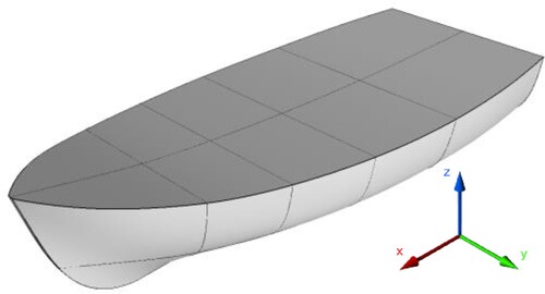
Figure 1 shows the position of Vertical Centre of Buoyancy (KB) and Gravity (KG). Each displacement (draught) has each vertical buoyancy (KB). From this condition, we also can calculate MB as a volume displacement function (MB = I/Vol). The total of both heights (KB + BM) is called KM. In this research, the influence of loading conditions (empty, half, and full load) is examined, as it can change the KM. Different KG was also examined and resulted in different MG, as MG = KM – KG. Changes in the load will affect the stability points such as KG, KM and GM, and alter the natural frequencies and damping coefficients in the roll and pitch motions of the ship. As a result, the ship's motion responses will also change. The coordinate system used in this study is shown in Figure 2.

Figure 1. Position of KM, KG, and GM.

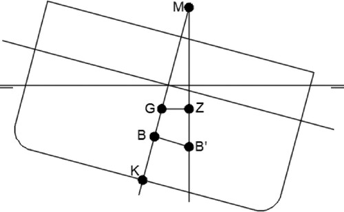
Figure 2. Coordinate system of the boat.

In this study, an operability analysis with a fishing boat was carried out to determine how the boat can operate safely and comfortably in its operational area, ensuring that the boat does not exceed the pre-determined seakeeping criteria. This investigation aims to inform the fishers of how long the boat should keep on standby on the shore until the weather conditions permit the boat to operate. In this work, a 5-metre-long traditional fishing boat operating in the Java Seas, Indonesia, was used as a case study. Five configurations of loading conditions were employed to represent the operation of the fishing boat in question. Each condition was then examined for its seakeeping performance and operability based on a 2-D linear potential theory using ShipX VERES Software.

Two types of operability assessment were utilised in this study, namely Percentage Operability (PO) developed by Fonseca and Soares (2002) and Operability Robustness Index (ORI) developed by Gutsch et al. (2020). PO was assessed corresponding to seakeeping criteria for fishing vessels. ORI was applied to evaluate the RMS roll response and the expected maximum roll amplitude of the boat, which were observed as key to preventing stability failure. The stability curve is used to relate the ship stability analysis to the seakeeping analysis.

This paper is organised as follows. Section 2 describes a literature review on the seakeeping method and operability analysis with some existing criteria. Subsequently, Section 3 illustrates ship geometry, load configuration and equilibrium condition. Following this, this research methodology is explained in Section 4. In Section 5, the results and discussion of this research are demonstrated. Lastly, Section 6 summarises the results of this study and some suggestions for future work are made.

2. Background

2.1. Overview of operability analysis

Sea conditions always change with time and depend on the location. To ensure the ship can be well operated within these conditions, long-term analysis is used, also called ship operability analysis. Ship operability is the percentage of time in which the ship can operate in an area by meeting selected seakeeping criteria based on an existing Wave Scatter Diagram (WSD). WSD is statistical data of waves in a particular location that records the number of occurrences of significant wave heights ($H_s$) and wave peak periods ($T_p$) within certain time ranges, such as daily, weekly, monthly, seasonal, and annually.

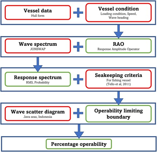
Figure 3 describes an overview of the operability analysis procedure. The red colour is an input for calculation, and the green colour is the result. First, vessel data and the conditions are required to calculate response amplitude operators (RAOs), the boat responses in regular waves. The combination between RAOs and selected wave spectrum will result in responses spectrum (short-term analysis), boat responses in irregular waves. The variance of the motions, such as root means square (RMS) and the probability, can be determined from the response spectrum. Then, the selected seakeeping criteria will result in operability limiting boundary, the limit of significant wave height and wave period that make the boat responses do not surpass the seakeeping criteria. Lastly, a particular wave scatters diagram of a specific sea area (the location where the boat operates) is used to calculate the percentage operability.

Figure 3. Overview of the operability analysis procedure.

2.2. Seakeeping analysis

From Figure 3, calculating a ship response in regular waves (RAO) is important to determine the operability analysis. The literature offers a wealth of seakeeping techniques which can be used to predict an RAO curve. One of the methods used to predict the motion responses of a ship is the 2-D Strip theory method which was introduced by (Salvesen et al. 1970). This method splits the underwater part of the ship into several strips. Analytical or numerical methods are used to solve the two-dimensional hydrodynamic problem for each strip. Three-dimensional effects are ignored assuming there is no interaction between the strips, reducing computational time. The forces and moments from each two-dimensional cross-section can be integrated along the ship length to calculate the total force. This method is widely used because it is fast and sufficiently accurate for conventional hulls. Even though strip theory is widely used, it has some limitations. The boat must be slender, and sail at low Froude numbers in relatively small waves, assuming first-order wave frequency motions only.

The development for solving the seakeeping problem evolved from 2-D to 3-D when computers become more advanced. The 3-D Panel Method can be used as an alternative to circumvent many of the assumptions made in the 2-D strip theory, for example, Datta et al. (2011). They investigated the fishing boat motion, where the hull form is not slender in the time domain. The 3-D Panel method requires the discretisation of the wetted surface into panels and some parts of the adjacent free surface. The hydrodynamic problem in each panel is solved using either the free-surface Green-function or Rankine panel method (He and Kashiwagi 2014). This method can solve the ship motion in the time domain, for example, Liapis and Beck (1985) used the green-function method for a constant forward speed and Beck and Liapis (1987) for a zero-speed problem. For Rankine panel method was initially presented by Nakos and Sclavounos (1991).

The Computational Fluid Dynamics (CFD) technique is another method used in seakeeping analysis. A ship can be simulated in regular waves to determine its motion response characteristics. The time-series results of ship responses are converted to the frequency domain results using Fourier Transform to obtain the RAO values (Tezdogan et al. 2016, 2015). One of the advantages of the CFD method is that the full-scale ship simulation for seakeeping performance and ship resistance can be modelled presented by several researchers, such as Tezdogan et al. (2015), Niklas and Pruszko (2019), and Ozturk et al.(2021). The CFD method is not only powerful to model regular waves but also irregular waves as described by Romanowski et al. (2019) and Zhang et al. (2021).

In this study, VERES, a plug-in of the ShipX software package was used to determine the ship RAOs. This method is based on the 2-D linear strip theory. The ship responses are assumed to vary linearly with incident wave amplitudes which are assumed to be small compared to the vessel dimensions. The wave steepness is also assumed to be small, so the waves are far from breaking. To determine the hydrodynamic forces, a potential theory is employed. The fluid is assumed as inviscid, irrotational, and incompressible. The viscous roll damping is determined from an empirical formula for roll motions. The components of this formula are frictional shear stress on the hull surface (Kato 1957), eddy damping (Ikeda et al. 1977), lift damping (Himeno 1981) and the bilge keel damping (Ikeda 1979). As the ship geometry considered in this study has no bilge keel, the latter component is not included.

2.3. Operability index

The methodology to calculate an operability index as the assessment of the seakeeping performance was presented by Fonseca and Soares (2002). In their study, two different types of vessels, container ship and fishing vessel were selected as a case study to evaluate the sensitivity analysis. Their type, mission and operational area are different resulting in different operability indexes. Moreover, the operability of four fully-loaded fishing vessels was investigated by Tello et al. (2009). From their research, it was revealed that roll motion and lateral acceleration had the lowest percentage operability among other responses. The boat with the ‘U’ type had a higher operability index than the ‘V’ type boat. It also can be inferred that the overall operability of fishing vessels had dependencies on the vessel’s dimension. The longest vessel can operate better compared to others, with the operability index of 0.94 for zero speed and 0.87 for Fr = 0.3. For the smallest vessels, the operability index was 0.44 and 0.64 for Fr = 0.0 and Fr = 0.3, respectively.

Furthermore, Tello et al. (2011) evaluated the seakeeping performance of a set of fully loaded fishing vessels operating in sea states 5 and 6. It was shown that pitch and roll were the most crucial degrees of freedom since their responses often surpass the limiting criteria. This research also mentioned that the GM is the essential parameter governing roll responses. The higher the GM of a vessel, the lower its roll period will be. As a consequence, the natural roll period may match with the wave modal period of the sea and lead to resonance. This will be dangerous since the roll responses will increase significantly and pose a danger to the vessel.

Tezdogan et al. (2014) investigated the percentage operability of a high-speed catamaran passenger ship using annual and seasonal WSD on the west coast of Scotland. This research was conducted using three theories to define the RAO curve; 2-D conventional strip theory (Theory 1) and high-speed strip theory formulation in 2½-D in which hull interaction between two hulls was not included (Theory 2) and was included (Theory 3). Those theories were then compared to the experimental data. The result of Theory 3 was closer to the experimental data compared to Theory 2. There was an enhancement in resonance frequency for heave motion when hull interaction was included. However, Theory 1 showed the best agreement with the experimental data among the three theories.

Recently, some researchers developed a new operability index showing a single seakeeping criterion, such as RMS roll. Gutsch et al. (2017) introduced the new performance indicator, namely the Integrated Operability Factor (IOF), defined as the ratio of the area below the curve of percentage operability for a single criterion from zero to its maximum limitation ($O{P}_{totmax}$) and the area of the maximum possible operability (100% $\times$ $O{P}_{totmax}$). In this case, the $O{P}_{totmax}$ of RMS Roll criterion was determined according to STANAG (Eriksen et al. 2000) for replenishment operations at sea, which is 2.2°. The work of Gutsch et al. (2017) investigated the change of some main dimensions of Offshore Construction Vessels (OCV), such as length, breadth, draught, transversal GM, and radius of gyration of roll (R₄₄) to the IOF value of RMS Roll.

Sandvik et al. (2018) used IOF for every single criterion of the RMS of heave, pitch, roll, and vertical crane displacement for the OCV. In their research, the combination of some main dimensions of the vessel was also investigated. They introduced this not only to operability analysis, but also to Relative Rate of Operation (RRO). Sandvik et al. (2018) further investigated the susceptibility of delay due to weather.

Later, Gutsch et al. (2020) changed the term IOF to Operability Robustness Index (ORI). Both IOF and ORI are the same analysis, which is the ratio between the two areas mentioned above. In their study, Gutsch et al used ORI as a key performance indicator (KPI) for the seakeeping performance of OCV. The sets of main dimensions were investigated to better understand the influence of length, beam, draught, and metacentric height when operating in the summer and winter seasons in North Sea and North Atlantic on the ORI value of RMS Roll. The $O{P}_{totmax}$ used here was 2°, which was then compared to the widely known PO.

From the study of Gutsch et al. (2020), it can be concluded that the ORI is the performance indicator that is more robust to assess the seakeeping performance of various vessel types. The higher ORI value is most affected by initial steepness from the curve of percentage operability and the choice of maximum limitation ($O{P}_{totmax}$) of the selected criterion (Sandvik et al. 2018). Nevertheless, although ORI can assess a single criterion of seakeeping performance, such as roll motion, this analysis is not related to the ship stability analysis.

2.4. Relationship between seakeeping and ship stability

One of the ship motion responses obtained from the seakeeping analysis is roll. This response is related to ship stability, defined as the ship's ability to keep returning to its original position due to roll motion caused by external disturbances. Ship accidents, such as capsizing, mostly occur due to stability failures. One of the reasons for capsizing is that ship operators are not given sufficient training regarding ship stability, so there are decision-making mistakes (Davis et al. 2019). To solve this problem, Caamaño et al. (2018) proposed a methodology to automatically assess the ship's stability to minimise the interaction between the crew and the system. This method can estimate the natural frequency of roll motion and the metacentric height throughout the vessel’s voyage. Later, Caamaño et al. (2019) proposed real-time detection of ship stability changes. The system lets the crew know how far the current situation is from the safety limit.

In a stability assessment, the scenario of loading condition is determined at the beginning to describe ship operation during the voyage. Then the characteristics of the stability curve of each loading condition are evaluated using standard criteria for fishing vessels based on the Intact Stability Code from IMO (2008). Mantari et al. (2011) investigated intact stability on fishing vessels involving fishing gear, beam waves, and wind. The results stated that the heeling moment produced by fishing gear is more critical than the heeling moment from bad weather scenarios. In addition, errors in choosing the dimensions of fishing gear and machines are also one of the factors for stability failure on fishing vessels.

However, current stability criteria may not accurately account for some of the dynamic phenomena in stability-related accidents (Mata-Álvarez-Santullano and Souto-Iglesias 2014). The ship's stability curve and its criteria recommended by IMO do not consider wave height and ship size. On this basis, the relationship between ship stability and safety to avoid capsizing was proposed by Deakin (2005). This research was conducted experimentally to determine the minimum wave height to capsize the ship for each configuration.

Deakin (2005) then produced a formula linking the stability curve represented by the range (angle distance that has a positive GZ) and the maximum Righting Moment (GZ max $\times$ displacement) with the size of the vessel which is represented by the length and width. Furthermore, the formula is refined by Deakin (2006) to determine the critical significant wave height or critical sea state. The influence of the ship's speed and the direction of the wave angle is not included in the formula. Meanwhile, with the same stability curve, the limiting wave height will be different depending on the vessel speed and the direction of the wave angle. The current study presents significant wave height limitations with vessel speed, and wave headings are considered.

In addition, research on the stability and operability of several sunken fishing vessels and several existing fishing vessels, which are similar to sunken vessels, was carried out by Mata-Álvarez-Santullano and Souto-Iglesias (2014). Stability and operability were investigated separately and not directly related. Stability analysis uses the stability index, which is the ratio of KG to the maximum allowed KG to meet the stability criteria. The operability was analysed using only short-term analysis, which was carried out on two typical sea states without considering WSD. The operability calculation differs from the percentage operability because it uses Boolean operators, choosing a value of 0 or 1 for each ship's speed and wave direction.

The researchers stated above tried to relate ship stability to the ship operability analysis. However, none have done so directly. Therefore, the present study aims to relate the seakeeping performance, especially roll motion, directly to the static stability of a vessel. For small boats, this relationship is considered to be crucial because the natural period of the roll is small, and it may coincide with the wave period leading to roll resonance. The novel indicator for seakeeping performance, ORI, was employed in the calculations not only for RMS of roll motion but also for the expected maximum roll. From the literature, the novelty of this research can be summarised as follows:

To date, no studies have analysed the operability of small vessels considering changes in loading conditions. Seakeeping analyses on fishing vessels are mostly done by comparing many vessels. Most of them only consider one loading condition, full load. This study analyses a single fishing boat, but the loading conditions are different. This is a characteristic of fishing vessel operations, where the cargo is constantly changing while underway. This study presents a comprehensive analysis to better understand the changes in cargo on fishing vessel operability.

Some researchers use the GM parameter in actual conditions to relate the ship's roll response. In fact, for the same hull, the GM value depends on the KM value, which varies depending on the ship's displacement. The ship's response will be different with the same GM value but different KM. Thus, the actual value of GM cannot directly determine the ship's response if it has a different KM. This study uses the GM/KM ratio to assess how GM and KM change and their influence on operability.

Several researchers have attempted to link ship stability with operability. However, none of these studies directly link ship stability and operability. This research offers a new idea to do this directly. The Angle of Vanishing Stability (AVS) and Downflooding Angle (DFA) in the stability curve is used as the maximum limitation (OPmax) of the expected maximum roll and then evaluated using ORI. This idea is based on the fact that if the maximum roll motion of the ship exceeds AVS, even if it occurs only once, the ship will become unstable because it has a negative GZ value. The ship has the potential to capsize because it has no righting moment. Moreover, when the maximum roll motion exceeds DFA, seawater is considered to enter the deck.

3. Ship geometry and conditions

In this paper, a traditional small fishing boat from Indonesia was selected as a case study. This fishing boat had been investigated by Tezdogan et al. (2018) earlier for optimisation of hull form and by Liu et al. (2019) for the design of a bilge keel. A body plan of the fishing boat is shown in Figure 4, and details of the main dimension are given in Table 2. The boat was simulated at three speeds, which are zero knots, half design speed (4 knots), and design speed (8 knots) with wave heading from 0° (heading wave) to 180° (following wave) with a 30° increment. The radius of gyration of the boat was obtained using Rhinoceros software, which are K_xx = 0.55 m, K_yy = 1.36 m, and K_zz = 1.43 m.

Figure 4. Body Plan of the Research Object (Liu et al. 2019).

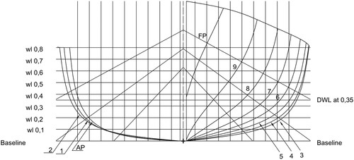
Table 2. Main Dimension of the Boat (Tezdogan et al. 2018).

Parameters	Value
Length between perpendicular, LPP (m)	5.000
Breadth at water line, B (m)	1.934
Depth to 1st deck, D (m)	1.196
Loaded draft, T (m)	0.350
Displacement, Δ(ton)	1.858
Block coefficient, Cb (-)	0.537
Mid-boat section coefficient, Cm (-)	0.764
Wetted surface area, Aw (m^2)	10.201
Froude number, Fr (-)	0.590

Aside from different velocities and wave headings, the boat was investigated with different loading conditions according to the scenario of fishing vessel operations, starting from Load Case 1 to Load Case 5 (Table 3). Load Case 1 is departure condition, where the fish storage tank is still empty because no fish has been caught. In Load Case 2, it is assumed that the vessel has caught half of the fish storage tank capacity, and the catch is placed on the upper deck. For Load Case 3, the catch is placed in the fish storage tank (below deck). Load Case 4 assumes that a total capacity of the fish storage tank has been caught and is placed on the upper deck, while Load Case 5 models this as below the deck. The details of Load cases 1–5 are shown in Table 3. It should be noted that the Transverse Centre of Gravity (TCG) is zero for all load cases since the load distribution is assumed to be symmetrical.

Table 3. Load Scenario.

Load Case	Description	Ship Weight (kg)	LCG (m)	KG (m)
1	Empty load of fish	712.00	1.550	0.844
2	Half load of fish, upper deck	1285.00	1.751	0.914
3	Half load of fish, below deck	1285.00	1.751	0.557
4	Full load of fish, upper deck	1858.00	1.828	1.064
5	Full load of fish, below deck	1858.00	1.828	0.57

To summarise, the vessel’s load capacity is divided into three conditions: empty, half, and the total capacity of fish storage. Each condition has a different loading position (KG) for both half and full capacities, so the centre of gravity is changed too. The different displacement and the centre of gravity will change along with the draft values for AP, FP and Midship locations and create the different trim conditions. The equilibrium condition of each load case can be seen in Table 4.

Table 4. Equilibrium Condition.

Parameters	LC 1	LC 2	LC 3	LC 4	LC 5
Displacement (kg)	712	1285	1285	1858	1858
KMt (m)	1.607	1.37	1.37	1.227	1.227
GMt (m)	0.763	0.456	0.813	0.163	0.657
Draft Amidships (m)	0.171	0.265	0.266	0.344	0.345
Draft at FP (m)	0.123	0.237	0.239	0.317	0.32
Draft at AP (m)	0.219	0.293	0.292	0.372	0.37
Draft at LCF (m)	0.185	0.272	0.272	0.35	0.349
Trim (+ve by stern) (m)	0.096	0.056	0.053	0.055	0.05
Trim angle (+ve by stern) (°)	1.0959	0.6391	0.608	0.6274	0.5743

With the same KM (as the boat's weight is the same), the GM will be different and affect the ship’s response, especially roll motion. There are differences in the natural period and damping values. This difference can be seen in the graph of the ship's response in regular waves, or what is commonly referred to as Response Amplitude Operator (RAO). The details of these results are discussed in depth in Section 5.1.

Figure 5 and Table 5 show the AVS and DFA for Load Case 1–5 in the stability curve, calculated by Maxsurf Stability Software. AVS is a static angle in the stability curve with zero GZ. In this condition, the ship is neither stable nor unstable. While DFA is a static angle, where the water meets any opening on the hull surface when calculating intact stability curve. The opening on the hull surface is marked with a downflooding point. However, in this study, the deck edge is defined as a downflooding point.

Figure 5. AVS and DFA of Load Case 1–5.

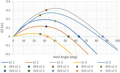
Table 5. AVS and DFA for Load Case 1–5.

Load Case	AVS (deg)	DFA (deg)
LC 1	63.15	40.35
LC 2	53.09	31.80
LC 3	85.98	31.80
LC 4	32.96	26.00
LC 5	82.27	26.00

A different displacement such as empty (LC 1), half (LC 2 & 3), and full load (LC 4 & 5) results in different DFA. The vertical shift of centre of Gravity (KG) with the same displacement does not influence the DFA. It only influences the AVS. However, even if AVS is the same, the GZ value for the same displacement is different. These results will influence the roll responses and operability performance.

4. Methodology

4.1. Ship response in regular wave

The RAO of a ship in regular waves is described as the ratio between the response output ($S_j$) to the wave excitation input ($\zeta$) for the six degrees of freedom (6DOF) in $j$ mode (for $j=1-6$), as a function of encounter wave frequency (${\omega }_e$), and wave heading ($\beta$), as shown in Equation 1. For rotational motion RAO, the wave excitation input ($\zeta$) is multiplied by wave number ($k$). (1) $RA{O}_j({\omega }_e\beta )={\displaystyle \frac{S_j(\omega \beta )}{\zeta (\omega )}}$(1)

4.2. Ship response in irregular wave

After the calculation of the responses of the ship in regular waves, short-term responses in irregular seas should be calculated. An irregular seaway is defined as the sum of the regular waves in which each wave has a random height and period (St Denis and Pierson 1953). A wave spectrum is used to represent a particular sea state. A short-term spectral analysis is used to predict the ship motions in a specific sea state. This analysis combines the transfer functions and the selected wave spectrum.

There are many standard wave spectra recommended by the International Towing Tank Conference (ITTC) (2002), such as spectra formulations given by Pierson Moskowitz (Pierson and Moskowitz (1964), ISSC (1964), ITTC (Mathews 1972), and Liu (1971)), JONSWAP (Hasselmann et al. 1973), Scott (1965), and Ochi and Hubble (1976). In this present study, a JONSWAP spectrum is used. The wave spectrum multiplied by the square of the RAO gives the response spectrum. The area under the response spectrum can be used to determine the variance of the motions in question.

The JONSWAP Spectrum was used in this study because it suits the conditions of the boat’s operational area (the Java Sea, Indonesia), which is closed waters or an archipelago (Hasselmann et al. 1973), (Djatmiko 2012). The JONSWAP spectrum formula is shown in Equation 2. (2) $S_{\zeta }(\omega )=\left[{\displaystyle \frac{\alpha g^2}{{\omega }^5}exp\left\{-{\displaystyle \frac{5}{4}{\left({\displaystyle \frac{{\omega }_p}{\omega }}\right)}^{-4}}\right\}}\right]{\gamma }^{exp\left\{-{\displaystyle \frac{{(\omega -{\omega }_p)}^2}{2{\sigma }^2{\omega }_p^2}}\right\}}$(2) where $\alpha =5.061(2\pi {)}^{-4}{H}_s^2{\omega }_p^4[1-0.287ln(\gamma )]$ is the normalisation factor, ${\omega }_p$ is modal wave frequency $(2\pi /T_p)$, $\omega$ is incident wave frequency, $\sigma =0.07$ is spectrum width parameter for $\omega \le {\omega }_p$ and $\sigma =0.09$ for $\omega >{\omega }_p$, and $\gamma$ is peakedness parameter which varies between 1.0–7.0. For Indonesian waters, $\gamma =2.0-2.5$ (Djatmiko 2012). In this study peakedness parameter, $\gamma =2.5$, was selected to calculate the highest sea condition.

The wave spectrum should be converted to a response spectrum $S_r(\omega )$ to analyze the ship’s response in irregular waves. The wave spectrum $S_{\zeta }(\omega )$ multiplied by the RAO squared gives the response spectrum $S_r(\omega )$, as shown in Equation 3. The area under the response spectrum curve is expressed by $m_n$ or the $n$-th moment (Equation 4), where $n=0$ for displacement, $n=2$ for velocity, and $n=4$ for acceleration. The square root of $m_n$ is called the Root Mean Square (RMS) or standard deviation, as shown in Equation 5. (3) $S_r(\omega )=RA{O}^2\times S_{\zeta }(\omega )$(3) (4) $m_n=\underset{0}{\overset{\mathrm{\infty }}{\int }}{\omega }^n{S}_r(\omega )d\omega$(4) (5) $RMS=\sqrt{m_n}$(5)

Ship responses are usually calculated at the Centre of Gravity (CoG). However, ship responses at other points of interests, such as the fore peak (FP) for deck wetness and slamming probability, should also be investigated. Both heaving and pitching responses at the CoG can be used to determine ship responses at the FP. This response is called absolute vertical motion at FP ($Z_{FP}$), as shown in Equation 6. (6) $\begin{array}{c}{Z}_{FP}={(Z_{FP})}_{a}cos({\omega }_{e}t+{\epsilon }_{FP})\\ {(Z_{FP})}_a=\sqrt{{(Z_a)}^2+{(x_{FP}{\theta }_a)}^2-2x_{FP}{Z}_a{\theta }_{a}cos({\epsilon }_{\theta }-{\epsilon }_Z)}\\ {\epsilon }_{FP}=ta{n}^{-1}\left({\displaystyle \frac{Z_{a}sin({\epsilon }_Z)-x_{FP}{\theta }_{a}sin({\epsilon }_{\theta })}{Z_{a}cos({\epsilon }_Z)-x_{FP}{\theta }_{a}cos({\epsilon }_{\theta })}}\right)\end{array}$(6) where $(Z_{FP}{)}_a$ is amplitude of absolute vertical motion at FP, ${\epsilon }_{FP}$ phase angle of absolute of vertical motion at FP, $Z_a$ and ${\theta }_a$ are the amplitude of heaving and pitching motions, $x_{FP}$ is longitudinal distance from CoG to FP, ${\epsilon }_Z$ and ${\epsilon }_{\theta }$ are the phase angle of heaving and pitching motions.

After the absolute vertical motion at FP has been determined, this response is calculated relative to wave amplitude at the FP to generate the RAO curve. This response is called relative vertical motion ($S_{FP}$), as shown in Equation 7. (7) $\begin{array}{c}{S}_{FP}={(S_{FP})}_{a}cos({\omega }_{e}t+{\epsilon }_s)\\ {(S_{FP})}_a=\sqrt{{({(Z_{FP})}_a)}^2+{({\zeta }_a)}^2-2{(Z_{FP})}_a{\zeta }_{a}cos(k{x}_{FP}-{\epsilon }_{FP})}\\ {\epsilon }_s=ta{n}^{-1}\left({\displaystyle \frac{{(Z_{FP})}_{a}sin({\epsilon }_{FP})-{\zeta }_{a}sin(k{x}_{FP})}{{(Z_{FP})}_{a}cos({\epsilon }_{FP})-{\zeta }_{a}cos(k{x}_{FP})}}\right)\end{array}$(7) where $(S_{FP}{)}_a$ is the amplitude of relative vertical motion at FP, ${\epsilon }_s$ is the phase angle of relative of vertical motions at FP, ${\zeta }_a$ is the wave amplitude, $k$ is the wave number.

Based on Equation 7, a different encounter frequency (${\omega }_e$) will produce different relative vertical motions at FP ($S_{FP}$). All encounter frequencies will generate another RAO graph, which is RAO for relative vertical motion at FP. Based on Equation 4, the response spectrum of motion and velocity ($m_0,m_2$) can be determined. Equation 8 and Equation 9 are used to calculate the Probability of Slamming and Deck Wetness. Here, $T$ is the draft in metres, $V_{cr}$ is the velocity threshold in m/s where $V_{cr}=0.093\sqrt{Lpp\times g}$, $Fb$ is the freeboard in metres, $m_0$ and $m_2$ are area under displacement and velocity response spectrum, respectively. (8) $P_{slamming}=exp\left\{-\left({\displaystyle \frac{T^2}{2m_0}+{\displaystyle \frac{V_{cr}^2}{2m_2}}}\right)\right\}$(8) (9) $P_{deckwetness}=exp\left\{-{\displaystyle \frac{F{b}^2}{2m_0}}\right\}$(9)

4.3. Operability limiting boundary

Seakeeping criteria are used to evaluate the vessels’ performance based on short-term spectral analysis. These criteria are essential as they can be used to determine a ship’s operability in a certain period by combining them with a Wave Scatter Diagram (WSD). Various types of seakeeping criteria exist today. These criteria are used according to the type of ships, such as the Nordic cooperative research project on the seakeeping performance of ships (NORDFORKS) for a merchant ship, naval vessel, and fast small craft (Nielsen 1987) and NATO Standardisation Agreement (STANAG) 4154 for naval vessels (Eriksen et al. 2000). For passenger ships, the criteria are more focused on passenger comforts, such as Motion Induced Interruption (MII) (Baitis et al. 1995) and Motion Sickness Incident (MSI) (O’Hanlon and McCauley 1973). Details for different types of seakeeping criteria can be found in Ghaemi and Olszewski (2017).

Sariöz and Sariöz (2006) investigated the seakeeping performance of high-speed displacement vessels (HSDVs) using typical seakeeping performance criteria. The pitch and roll motions, vertical and lateral accelerations, and the number of slamming events and deck wetness per hour were found to be significant in determining the seakeeping criteria. For a high-speed passenger ship, Tezdogan et al. (2014) used human comfort as limiting criteria which are MII, MSI, vertical and lateral accelerations. In the current study, the limiting criteria are selected for fishing vessels listed in Table 6 (Tello et al. 2011).

Table 6. Seakeeping Criteria for Fishing Vessel (Tello et al. 2011).

No	Criteria	Limit
1	RMS roll	6.00°
2	RMS pitch	3.00°
3	Probability of green water (GW)	0.05
4	Probability of slamming (SL)	0.03
5	RMS vertical acceleration at working area / bridge deck (VA)	0.20 g
6	RMS lateral acceleration at working area / bridge deck (LA)	0.10 g

Each criterion has a different operational limit, meaning that each criterion has a different maximum significant wave height as a limitation for the vessel to operate for a certain peak wave period. Nevertheless, all criteria must be met to set the limits of the vessels’ operation.

The ship response per metre of significant wave height ($g_x$) can be written as in Equation 10 which ${\sigma }_x$ is ship response and $H_s$ is significant wave height. For displacement/motion criteria, Equation 11 is used to determine the limiting of a significant wave height ($H_s^{lim}$), where ${\sigma }_x^{lim}$ is the limiting value of the specific motion criterion. (10) $g_x={\displaystyle \frac{{\sigma }_x}{H_s}}$(10) (11) $H_s^{lim}(T_p)={\displaystyle \frac{{\sigma }_x^{lim}}{g_x}}$(11) While for the slamming criterion, Equation 12 is used to determine the limiting significant wave height ($H_s^{lim}$), where $Ps$ is a probability of slamming criterion ($Ps$  = 0.03), $g_r$ and $g_{rv}$ are RMS–value of relative vertical motion and velocity per metre significant wave height, respectively. The limiting significant wave height ($H_s^{lim}$) for green water criterion is shown in Equation 13, where $Pgw$ is a probability of green water criterion ($Pdw$  = 0.05). (12) $H_s^{lim}(T_p)=\sqrt{-{\displaystyle \frac{1}{2\ln Ps}\left({\displaystyle \frac{T^2}{{(g_r)}^2}+{\displaystyle \frac{V_{cr}^2}{{(g_{rv})}^2}}}\right)}}$(12) (13) $H_s^{lim}(T_p)={\displaystyle \frac{Fb}{g_r\sqrt{-2\ln Pdw}}}$(13)

4.4. Percentage operability

The operational area of a fishing boat is the Java Sea, located in the north of Java Island, Indonesia (Figure 6). The Annual WCS data can be seen in Table 7 obtained from metoceanview (https://app.metoceanview.com/hindcast/). As shown in Table 7, the highest percentage of wave period occurrences is 3–4 s with a percentage of 35.3% and 4–5 s with a percentage of 37.0%. The highest percentage for a significant wave height is 0.5-1.0 m with 45%, followed by 0.0-0.5 m with 39.8%, and 1.0-1.5 m with 13.3%. These waters can be categorised as sea state 3. In these conditions, a ship must have an operational limit over 1.5 m for all criteria to operate at least 98% of the time.

Figure 6. Location of Wave Scatter (www.bing.com/maps).

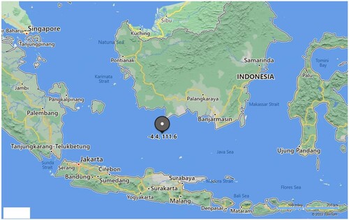
Table 7. Wave Scatter Diagram (https://app.metoceanview.com/hindcast/).

Hs (m) \ Tp (s)	0–1	1–2	2–3	3–4	4–5	5–6	6–7	7–8	8–9	9–10	Hs Occurrence
0.0–0.5	6	139	8192	25249	7677	518	48	21	3	0	39.8%
0.5–1.0	0	0	3	11863	28587	6764	88	6	0	0	45.0%
1.0–1.5	0	0	0	0	2650	10558	801	13	0	0	13.3%
1.5–2.0	0	0	0	0	0	840	830	32	0	0	1.6%
2.0–2.5	0	0	0	0	0	4	188	77	0	0	0.3%
2.5–3.0	0	0	0	0	0	0	6	52	1	1	0.1%
3.0–3.5	0	0	0	0	0	0	0	4	6	0	0.0%
3.5–4.0	0	0	0	0	0	0	0	0	0	0	0.0%
4.0–4.5	0	0	0	0	0	0	0	0	0	0	0.0%
4.5–5.0	0	0	0	0	0	0	0	0	0	0	0.0%
Tp Occurrence	0.0%	0.1%	7.8%	35.3%	37.0%	17.8%	1.9%	0.2%	0.0%	0.0%	100%

The percentage operability for a particular wave heading, seakeeping criteria, and ship speed is obtained by Equation 14. $P_{Op}^{\beta }$ is percentage operability for a particular wave heading, seakeeping criterion, and ship speed. $P_{jk}$ $(H_{s{j}_j}<H_{s_{cr}},T_k)$ is the probability of occurrence of a significant wave height in interval $j$ below the limiting significant wave height with a wave period in interval $k$. (14) $P_{Op}^{\beta }=\sum _{j=1}^{N_{Hs}}\sum _{k=1}^{N_{Tp}}{P}_{jk}(H_{sj}<H_{s_{cr}},T_k)$(14) The percentage operability for all headings with a certain seakeeping criterion and ship speed is obtained by Equation 15. $P_{Op}$ is percentage operability for all headings with a certain seakeeping criterion and ship speed. $P_{O{p}_i}^{\beta }$ is the percentage operability for the ith wave heading. $P({\beta }_i)$ is the probability of occurrence of the ith wave heading βi. If $P({\beta }_i)$ has an equal probability, then Percentage Operability for all heading can be calculated as average of Percentage Operability for all heading βi. (15) $P_{Op}=\sum _{i=1}^{N_{\beta }}{P}_{O{p}_i}^{\beta }P({\beta }_i)$(15)

4.5. Operability robustness index for roll motion

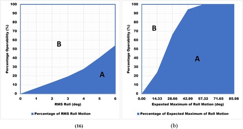
From Equation 16 and Figure 7a, the Operability Robustness Index (ORI) can be described as a ratio of the area below the curve of Percentage Operability of Roll motion criteria from 0° to 6° ($P_{op}(O{P}_{tot})$ or Area A) to the area of maximum theoretically possible operability ($O{P}_{totmax}\times 100$ or Area A + Area B). In this case, $O{P}_{totmax}$ is 6°, which is a limiting criterion of RMS Roll motion for a fishing vessel, as described in Table 6. (16) $ORI={\displaystyle \frac{{\int }_0^{O{P}_{totmax}}{P}_{op}(O{P}_{tot})d(O{P}_{tot})}{O{P}_{totmax}100}={\displaystyle \frac{AreaA}{AreaA+AreaB}}}$(16) An RMS roll motion of 6${}^{\circ }$ as a seakeeping criterion is a limitation to ensure the boat is safe and comfortable to be operated. Nevertheless, it is unknown if the boat will remain safe upon surpassing this limit. This present study utilises AVS and DFA to relate ship operability analysis to ship stability and to indicate whether the boat remains safe.

Figure 7. Definition of ORI for RMS Roll Motion (a), and Expected Maximum of Roll (b).

The expected maximum is defined as the maximum roll response that can be reached by vessel in a particular range of time, operated in a particular sea state. Rayleigh probability function is employed as an approximation to the probability density function for the maximum of the responses. Equation 17 is used to determine the single amplitude of the expected maximum of Roll Motion. (17) $\begin{array}{c}{E}_{max}Roll=\sqrt{m_{0}Roll}\left[\sqrt{2\ln N}+{\displaystyle \frac{0.5772}{\sqrt{2\ln N}}}\right]\\ N={\displaystyle \frac{T.3600}{T_{z}Roll}}\\ T_{z}Roll=2\pi \sqrt{{\displaystyle \frac{m_{0}Roll}{m_{2}Roll}}}\end{array}$(17) where $E_{max}Roll$ is expected maximum roll motion, $T$ is duration in hours. In this research, $T=3$ hours to illustrates the boat operate. $T_{z}Roll$ is the zero–up crossing period of the roll response.

According to Figure 7b, the vessels must have 100% operability, at least at maximum limitation angle, $O{P}_{totmax}$. In this case $O{P}_{totmax}$ is Angle of Vanishing Stability (AVS). If the boat has not been capable of being operated 100%, there is a chance for a boat to reach an angle of roll response higher than $O{P}_{totmax}$. The boat will have a negative GZ. It will be better if the vessel has 100% operability at the angle lower than $O{P}_{totmax}$. The value of ORI will increase excessively since area A in Figure 7 increases.

5. Results and discussion

5.1. Response amplitude operator

Each wave heading and boat speed results in a different RAO. Figure 8 shows the heave RAO graph at 0, 4, and 8 knots for head seas. It is known that the vertical motions are more pronounced in this heading. It should also be noted that in this study 0° wave heading corresponds to a head wave condition.

Figure 8. Heave RAO in Head Seas (0°) at 0 knot (a), 4 knot (b), and 8 knot (c).

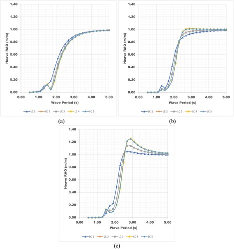
As shown in Figure 8, the peak of RAO increases along with the boat speed. The trend of curves is also similar to the boat displacement and Longitudinal Centre of Gravity (LCG), as shown in Table 3. The highest peaks of RAO belong to the load cases with the highest displacements (LC 4 and LC 5) and so for the next lower peak. It can be inferred that the boat displacement influences the heave damping, resulting in different heave motions.

The natural period of heaving motion also can be seen in Figure 8, where the period at the abscissa reaches the peak of the curve. For all load cases, the natural periods are similar to each other. This happens for a wave period between 2 and 3 s. Examining the WSD data in Table 7, the most frequent periods are 3–4 s and 4–5 s. However, 2–3 s wave periods have a 7.8% probability, indicating heave resonance can occur and increase the heave response.

Pitch RAO can be seen in Figure 9 for the three speeds: 0, 4, and 8 knots. LC1 at zero speed has a higher peak than the 4-knot speed at a wave period of about 3 s. LC 4 is the highest peak at zero speed, but it is not the only one for 4 and 8 knot speed; LC 5 is the highest too for both speeds.

Figure 9. Pitch RAO in head seas (0°) at 0 knot (a), 4 knot (b), and 8 knot (c).

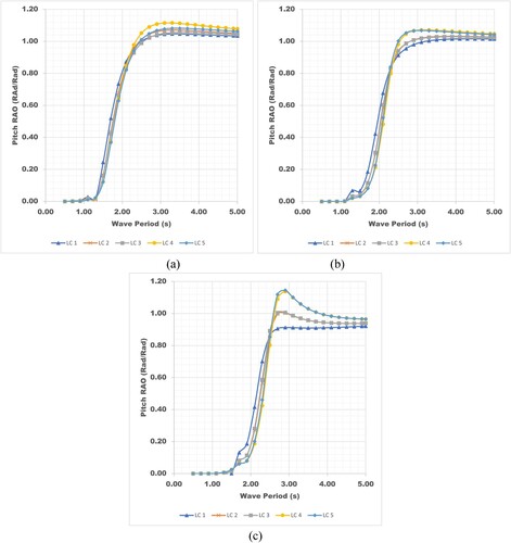
However, the trend of the pitch RAO peaks at 4 and 8 knots are likely similar to those of heave. The two highest are LC 5 and LC 4, and the lowest is LC 1. The pitch RAO peaks represent the effect of the damping coefficient. It can be concluded that the trend of damping coefficients for both speeds is similar to that of heave but not at zero speed. From Figure 9, we can also see that the natural period in pitch is similar to that in heave. The natural period for each speed and load case is about 2–3 s. It will also cause resonance in pitch, especially when the pitch damping is low. The pitch response will be significantly increased.

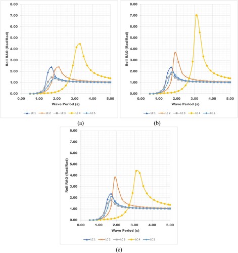
Figure 10 illustrates the roll RAO at 0, 4, and 8 knots. In this RAO, the beam sea (90°) was chosen since this heading most affects the ship's roll response. The peak of roll RAO varies with speed. LC 4 shows that the highest peak occurs at 4 knots, not at 8 knots. However, the higher the KG position, the higher the RAO peak, meaning a decrease in roll damping and an increase in roll response. It can be inferred that the determination of KG position is essential since it directly influences the roll response.

Figure 10. Roll RAO in Beam Seas (90°) in 0 knot (a), 4 knot (b), and 8 knot (c).

As shown in Table 4, each displacement has a different KM value. Different KG positions will result in different GM values with the same KM (GM = KM – KG). This is shown for LC 2 with LC 3 (half load) and LC 4 with LC 5 (full load). If we compare GM with each KM value, we can calculate the ratio of GM to KM, as shown in Figure 11.

Figure 11. Ratio KG and GM to KM.

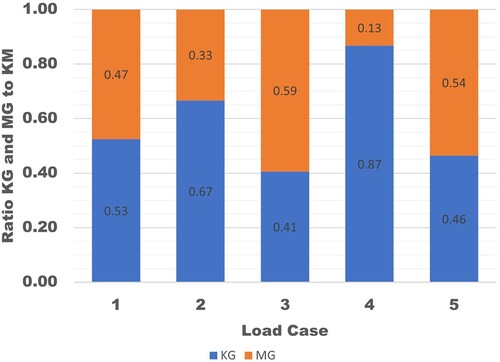
Based on Figure 10, LC 4, LC 2, and LC 1, a few different KG values (about 0.1 m) will result in a different ratio GM/KM because those LCs have a different KM. The GM/KM ratio value aligns with the RAO peak. So, the higher GM/KM ratio is, the lower RAO peak.

Unlike heave and pitch, Figure 10 shows that loading conditions, due to the change in the KG position, affect the natural roll period of the vessel. The natural roll period for LC 4, around 3 s, is considerably different from the other load cases, which show a natural roll period of 1–2 s. From WSD shown in Table 7, it can be seen that LC 4 is dangerous in roll resonance. The natural roll period is the same as the second most frequent period, 3–4 s, whose probability of occurrence is 35.3%. Other load cases (natural period of 1–2 s) do not significantly influence the roll resonance because the probability of occurrence is only 0.1%.

5.2. Operability limiting boundary

In Figure 12, the results of the operability limiting boundary for five load cases in wave heading of 60° at 8 knots are given. VA, LA, GW, and SL refer to Vertical and Lateral Acceleration, Green water, and Slamming. In the figure, the horizontal axis is the peak period. The vertical axis is a limit of significant wave height, where the boat responses do not exceed the seakeeping criteria. Each peak period has a different limitation of significant wave height. The ‘No Wave’ line is a border showing the breaking wave limit. This theoretical limit of breaking waves is shown in Equation 18. (18) $H_{BW}=0.105T_p^2$(18) where $H_{BW}$ is limit of breaking wave (m), $T_p$ is peak period (sec).

According to Figure 12, for all load cases, the limit of significant wave height for green water and slamming probability criteria are above the ‘No Wave’ line. This means, the boat would not surpass these two seakeeping criteria for all wave periods and significant wave height combinations and can be fully operated (PO is 100%).

On the other hand, the trough of the other four criteria lies below the ‘No Wave’ line when Tp > 2 s. Between 2–4 s, some criteria have the limits of significant wave height of one metre, while the others are a half metre. From WSD data in Table 7, it can be seen that the probability of occurrence for Hs with no more than a half metre is 39.8% for the total peak period. This result suggests that the boat has a low PO. Details of the results of percentage operability are described in the following section.

Examining Figure 12, the limiting significant wave heights are different for each load case. Overall, all load case has a limiting significant wave height below one metre. Referring to the limiting significant wave height based on the formula from Deakin (2006, 2005), the boat in this study has a limiting significant wave height below one metre. The results from this study are in line with Deakin’s. However, this study reveals which wave period results in low limiting significant wave height.

5.3. Percentage operability (PO)

PO results for three speeds, seven wave headings, and five load cases are listed in Figures 12–15. The probability of occurrence for each wave heading is considered equal. Thus, based on Equation 15, an average of all wave headings is defined as the PO for all headings.

Figure 12. Operability limiting boundary in wave heading 60°, at 8 knots for Load Case 1 (a), Load Case 2 (b), Load Case 3 (c), Load Case 4 (d), Load Case 5 (e).

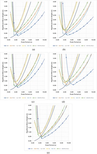
Figure 13. Percentage Operability for Criterion 1 and Criterion 2.

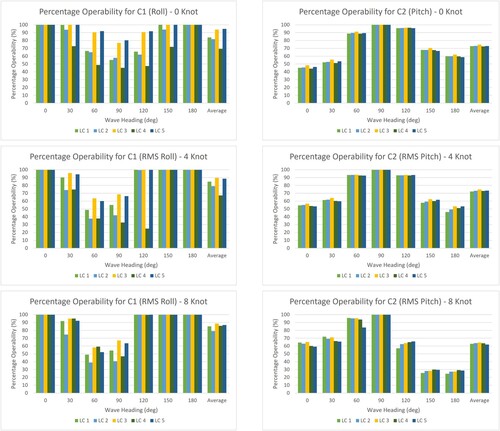
Figure 14. Percentage Operability for Criteria 3 and Criteria 4.

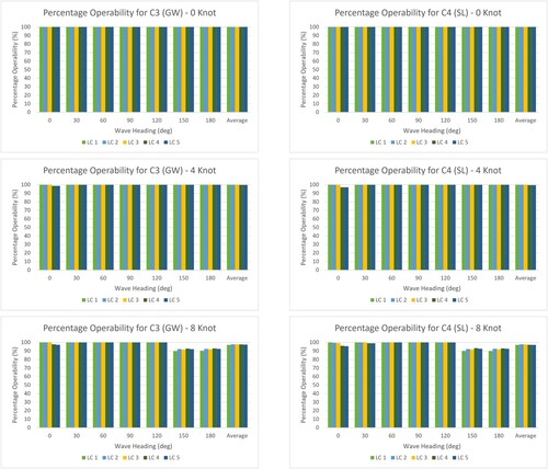
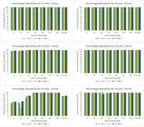
Figure 15. Percentage Operability for Criteria 5 and Criteria 6.

Figure 13 shows the percentage operability for Criterion 1 (RMS Roll) and Criterion 2 (RMS Pitch). The PO for Criterion 1 reaches low values in wave heading of 60°, 90°, and 120° for all speeds except at 8 knots, which can be operated well (100%) at 120°. Load Case 4 is the worst operability at zero speed and four knots. Contrary to 8 knots, Load Case 2 is the lowest value for the RMS roll criterion. According to Figure 11, Load Cases 2 and 4 have a minimum GM/KM ratio than other load cases, meaning that the roll damping is low, and hence the roll response is higher than in other cases.

The low PO for pitch criterion belongs to wave heading of 0°, 30°, 150° and 180° (head, quarter, and following waves). For 8 and 4 knots, the lowest PO occurs in following waves (180°) and quarter-following waves (150°), while the opposite is true in the zero speed case where this occurs in head waves (0°). For every speed, an average of PO for each load case has a similar value.

Figure 14 illustrates the PO for Criterion 3 (Probability of Green Water) and Criterion 4 (Probability of Slamming). It can be concluded that almost all speeds and load cases have excellent operability. A one hundred per cent operability is found at zero ship speed. At 4 knots, Load Cases 4 and 5 have the lowest operability value in a heading wave (0°), which is around 97-98%. For the maximum speed, the lowest operability value does not occur inhead wave but quarter following waves (150°) and following waves (180°). However, the value is no less than 89.9%. For both criteria, this value is sufficiently high for safe operations.

PO for Criterion 5 (vertical acceleration) and Criterion 6 (lateral acceleration) are shown in Figure 15. According to Criterion 5, the boat can be operated well for all load cases at zero speed. For Criterion 6, the lowest operability value is around 99%, occurring in head waves. The PO for criterion 5 in wave heading 0° and 30° have the lowest value in maximum speed, varying from 35% to 63%. This value is not high enough to operate the boat safely. For a 60° heading, the PO value is around 78% to 87%, whereas in the case of criterion 6, the lowest operability value occurs in heading 60° and 90°, above 91.9%.

The minimum PO values between criteria 1 and 6 are selected as the PO for all criteria, as shown in Figure 16. For wave headings of 60° and 90°, RMS roll is selected as PO for all criteria. For other wave headings, RMS Pitch is selected. For the highest speed, the operability for all load cases varies from 61% to 64%. For medium speed and zero speed, the operability is around 67% to 74%. Overall, the PO of this boat is relatively small. The boat cannot be operated safely in the Java Sea because some combinations of significant wave heights and wave peak periods do not meet the RMS roll and pitch limiting criteria.

Figure 16. Percentage Operability for All Criteria.

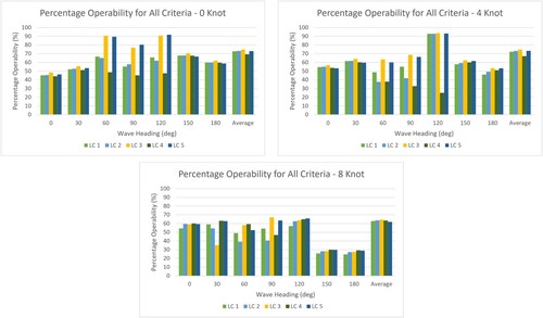
Based on Figure 13, with the low PO value, the RMS roll is predicted will surpass 6°. However, the maximum roll response experienced by the boat is still unknown until the analysis of the expected maximum roll is carried out.

Figure 17 presents the PO for the expected maximum of roll motion, with AVS (left-hand side) and DFA (right-hand side) as a limiting angle, given in Table 5. The left-hand side shows that almost all load cases have 100% PO, except LC 4. Based on these results it can be concluded that the boat can operate well in all cases except under the condition of LC 4. It should be noted that 100% of PO here means that the boat can operate without having a negative GZ, as the roll response is predicted not to exceed AVS. From this case, the different limiting angle (AVS) does not give a clear difference between the load case to the PO value.

Figure 17. Percentage Operability for Expected Maximum of Roll with a different limiting angle.

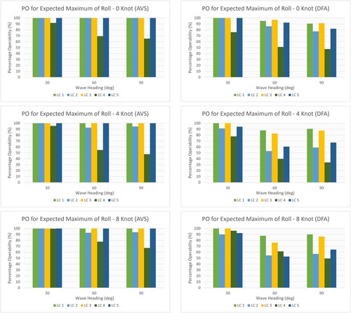
On the right-hand side of Figure 17 (with DFA as a limiting angle), it can be observed that each loading case results in a unique PO value. Since the DFA is lower than AVS, the calculation of PO becomes more sensitive to loading conditions even if the same limiting angle is used. This makes the distinction between load cases clearer.

Consequently, as LC 1 has the highest limiting angle (DFA), the PO of LC 1 is the highest. With DFA as a limiting angle, LC 1, LC 3, and LC 5 no longer have 100% operability like those from AVS. From this comparison, the choice of DFA as a limiting angle to calculate PO is better than AVS because this angle is more sensitive and clearly shows the distinction between the load case. It also should be noted that 100% of PO, in this case, means that the boat can operate without the edge of the deck meeting the water.

5.4. Operability robustness index (ORI) for roll motion

5.4.1. ORI for RMS roll motion

ORI is an operability index to assess a particular criterion. In this study, the chosen maximum limiting angle ($O{P}_{totmax}$) criterion for RMS roll is referred to Tello et al. (2011), which is 6°, as shown in Table 6. For each angle, the PO was calculated and plotted as a curve. The area below the curve is calculated as shown in Equation 16. In this research, angles from zero to the maximum limitation angle ($O{P}_{totmax}$) are divided into six angles to employ Simpson Rule for calculating the area below the curve. This area is then compared to the maximum area of the possible PO (100% $\times$ $O{P}_{totmax}$).

In Figure 18, the ORI results of RMS roll motion for all load cases in wave heading 30°, 60°, and 90° are presented. All loading condition attain their highest ORI value for a wave heading of 30°. This heading does not influence the roll motion as much as the others. Overall, LC 2 and LC4 have the lowest value compared to other load cases, except for LC 4 at maximum speed with a wave heading 60°. It can be concluded that it will be perilous for the fishermen to put the caught fish above the deck during the operation under the LC 2 and LC 4 conditions, especially when they catch the fish in large quantities at once, as it will suddenly influence the roll response of the boat.

Figure 18. Operability Robustness Index (ORI) Value for RMS Roll Motion.

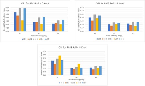
If the ORI results in Figure 18 are compared with the PO for the RMS roll in Figure 13, it can be seen as a clear view of why the ORI results are more objective than the PO results. PO values for LC 2 and LC 4 at 4 knots with a wave heading of 30° are similar, 74% and 74.80%, respectively. However, the ORI values for both load cases are different, 0.31 and 0.38. For the wave heading of 60°, PO values for LC 2 and LC 4 are also similar, specifically 37.70% and 37.90%. However, the ORI results are different, 0.17 and 0.21. From that example, it can be concluded that ORI approaches its maximum value slower than the PO value, and, therefore, allows boat designers and operators to rank performance independently of the chosen limiting criterion with a similar PO.

As explained by Gutsch et al. (2020), in comparison to PO, ORI accounts for the development of the PO value on its complete course of its behaviour between zero and the chosen maximum motion limitation. Gutsch et al. further conclude that ‘therefore, the ORI behaves qualitatively similar but approaching its maximum possible value of 1.0 slower. Consequently, the ORI allows vessel performance assessment to be more independent of the chosen environmental condition and level of limitation criteria.’

5.4.2. ORI for expected maximum of roll motion

The ORI of the expected maximum of roll motions are presented in Figure 19 for all load cases and speeds with wave headings of 30°, 60°, and 90°. Different $O{P}_{totmax}$, AVS and DFA, were examined as shown in Table 5. Angles from zero to maximum limitation angle ($O{P}_{totmax}$) are also divided into six angles to employ Simpson Rule for calculating the area below the curve.

Figure 19. Operability Robustness Index (ORI) Value for Expected Maximum Roll Motion with different maximum limiting angle.

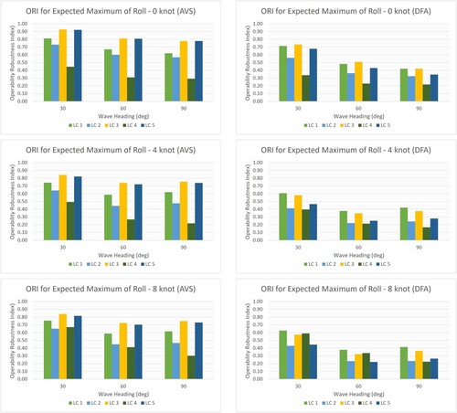
AVS as a $O{P}_{totmax}$ is presented on the left-hand side of Figure 19. Each load case has a different AVS which results in a different ORI. This difference cannot be seen by examining PO results (Figure 17). Based on the figure, for almost all conditions, the ranking of ORI values from best to worst is LC 3, LC 5, LC 1, LC 2, and LC 4. The order is different for 8-knots speed with a wave heading of 30°, where ORI for LC 4 is higher than LC 3 with a slight difference. The order of ORI results from the left-hand side of Figure 19 is aligned to GM/KM ratio in Figure 11 and the AVS from Table 5. Specifically, higher GM/KM ratios give better ORI values.

The ORI indicator gives a new perspective to better assess better Load Cases in seakeeping performance, especially in roll motion with the same PO of 100% (LC1, LC 3, and LC 5). When using AVS as a limiting angle, LC 3 is the best scenario for other load cases. This load case also has the highest GM/KM ratio, namely 59%. Under these conditions, the response of the roll motion becomes low, as seen from the Roll RAO in Figure 10.

On the other hand, when DFA is set as a $O{P}_{totmax}$ (right-hand side of Figure 19), all ORI values become lower than AVS. The reason is that the DFA is lower than AVS. In these cases, the limiting criterion became stricter, so the PO value also decreased (Figure 16). From the right-hand side of Figure 16, the PO of expected maximum of roll for LC 1 and LC 3 with a wave heading of 30° is 100%. The ORI results also allow boat designers or boat operators to distinguish and rank them. For zero speed, LC 3 is better than LC 1. For medium and maximum speed, LC 1 is better than LC 3.

As shown in Figure 19, even though ORI can rank all load cases, with different $O{P}_{totmax}$ (AVS and DFA) the order of load cases are different from top to bottom. This becomes clearer at the medium and maximum speeds. For example, Figure 20 explains why there is a different order of ORI values between LC 4 and LC 5 at maximum speed with a wave heading of 60°.

Figure 20. ORI calculation for same load case with different maximum limiting angle (AVS and DFA).

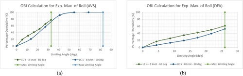
Based on Figure 20a, the maximum limiting angle (AVS) of LC 4 (32.96°) is lower than LC 5 (82.27°). At the low limiting angles, the PO of LC 4 is higher than LC 5. However, because LC 5 has a higher limiting angle and 100% PO at last limiting angles, LC 5 has a higher ORI that LC 4. When DFA is employed as a maximum limiting angle (Figure 20b), which is 26° for both load cases, the ORI results show that LC 4 is higher than LC 5.

This comparison shows that the ORI value is not only influenced by the maximum limiting angle ($O{P}_{totmax}$) but also the value of PO in each limiting angle. The lower $O{P}_{totmax}$ does not always make the ORI value lower. The PO value in each limiting angle also contributes to increasing the ORI value because the area below the curve is calculated from the PO value.

6. Conclusion

In this study, an operability assessment, both in Percentage Pperability (PO) and Operability Robustness Index (ORI), was carried out under different loading conditions. Different loading conditions give different GM/KM ratios as the position of KG changes. This ratio influences the roll responses and dampings, as shown in roll RAOs, but does not noticeably affect heaving and pitching motion, as the LCG is not influenced significantly.

The operational area of the boat, which can be categorised as sea state 3, gives low PO, especially in the peak period of 1–3 s. The PO of the boat for all criteria is not high, varying from 61% to 74%. Among all criteria, the limiting boundary for Criteria 1 (RMS Roll motion) and Criteria 2 (RMS Pitch Motion) renders the PO value low.

The PO for RMS roll motion is low because it exceeds 6° as a maximum limitation. This situation might make the crew uncomfortable on board, but it does not mean that the boat is unsafe. Therefore, an expected maximum of roll motion investigation was carried out to ensure the roll responses do not surpass the AVS. Thus, the GZ value is always positive. Once the GZ value becomes negative, the boat will be unstable and capsize. DFA was also employed as another limiting angle to investigate whether the expected maximum of roll will exceed DFA. If so, the deck edge will meet the seawater and the water is assumed to be on the deck.

Based on the PO for the expected maximum of roll motion, LC 4 is the worst scenario for all speeds and headings (for AVS chosen as $O{P}_{totmax}$). LC 2 is the same for medium and maximum speeds with wave headings of 60° and 90°. While other load case has 100% operability, which means the maximum roll response do not surpass the AVS. The boat is predicted to be stable and has a positive GZ.

On the other hand, the PO results are different for DFA as $O{P}_{totmax}$. Some load cases no longer have 100% operability like those from AVS. The expected maximum roll of the boat was predicted will exceeding DFA. From this comparison, the choice of DFA as a limiting angle to calculate PO is better than AVS because this angle is more sensitive and clearly shows the distinction between the load cases. Among load cases with 100% operability for the expected maximum of roll motion, an ORI investigation was carried out to assess which Load Case is better. A different $O{P}_{totmax}$ will give different results of ORI.

A loss of stability due to restoring moment variations when the wave profile is taken into account, such as parametric roll and pure loss of stability, is a part of our future work. The roll responses of a fishing boat from the head and following waves will be investigated using an unsteady Reynolds-Averaged Navier Stokes-based Computational Fluid Dynamics (CFD) technique. This technique will enable researchers to include the effect of the full nonlinearity and coupled heave, pitch, and roll motions.

Acknowledgement

The work published in this paper is drawn from the first author's PhD thesis. The first author gratefully acknowledges Diponegoro University in Indonesia for giving a PhD scholarship to support his study at the University of Strathclyde, Glasgow.

Disclosure statement

No potential conflict of interest was reported by the author(s).

References

- Baitis AE, Holcombe F, Conwell S, Crossland P, Colwell J, Pattison J, Strong R. 1995. Motion Induced Interruption (MII) and Motion Induced Fatigue (MIF) Experiments at the Naval Biodynamics Laboratory.
- Bappenas. 2010. Presidential Regulation No. 5 of 2010 concerning the National Medium-Term Development Plan (in Indonesian).
- Beck RF, Liapis S. 1987. Transient motions of floating bodies at zero forward speed. J Ship Res. 31:164–176.
- Caamaño LS, Galeazzi R, Nielsen UD, González MM, Casás VD. 2019. Real-time detection of transverse stability changes in fishing vessels. Ocean Eng. 189:106369.
- Caamaño LS, González MM, Casás VD. 2018. On the feasibility of a real time stability assessment for fishing vessels. Ocean Eng. 159:76–87.
- Datta R, Rodrigues JM, Soares CG. 2011. Study of the motions of fishing vessels by a time domain panel method. Ocean Eng. 38:782–792. doi:10.1016/j.oceaneng.2011.02.002.
- Davis B, Colbourne B, Molyneux D. 2019. Analysis of fishing vessel capsizing causes and links to operator stability training. Saf Sci. 118:355–363.
- Deakin B. 2005. An experimental evaluation of the stability criteria of the HSC Code, in: International Conference on Fast Sea Transportation, FAST.
- Deakin B. 2006. Developing simple safety guidance for fishermen, In: 9th International Conference on Stability of Ships and Ocean Vehicles, Rio de Janeiro, Brasil.
- Djatmiko EB. 2012. Behavior and operability of marine buildings on random waves (in Indonesian). Surabaya. Indones: ITS-Press.
- Domeh V, Obeng F, Khan F, Bose N, Sanli E. 2021. Risk analysis of man overboard scenario in a small fishing vessel. Ocean Eng. 229:108979.
- Eriksen JH, Nona RA, Mas C. 2000. Common procedures for seakeeping in the ship design process. STANAG 4154, 2000.
- FAO. 2000. The State of World Fisheries and Aquaculture Part 2: Selected Issues Facing Fishers and Aquaculturists, the State of World Fisheries and Aquaculture. Food & Agriculture Org.
- Fonseca N, Soares CG. 2002. Sensitivity of the expected ships availability to different seakeeping criteria, in: International Conference on Offshore Mechanics and Arctic Engineering. pp. 595–603.
- Ghaemi MH, Olszewski H. 2017. Total ship operability –review, concept and criteria. Pol Marit Res. 24:74–81.
- González MM, Sobrino PC, Álvarez RT, Casás VD, López AM, Peña FL. 2012. Fishing vessel stability assessment system. Ocean Eng. 41:67–78.
- Gutsch M, Sprenger F, Steen S. 2017. Design parameters for increased operability of offshore crane vessels, in: International Conference on Offshore Mechanics and Arctic Engineering. p. V009T12A029.
- Gutsch M, Steen S, Sprenger F. 2020. Operability robustness index as seakeeping performance criterion for offshore vessels. Ocean Eng. 217:107931.
- Hasselmann K, Barnett TP, Bouws E, Carlson H, Cartwright DE, Enke K, Ewing JA, Gienapp A, Hasselmann DE, Kruseman P, Meerburg A. 1973. Measurements of wind-wave growth and swell decay during the Joint North Sea Wave Project (JONSWAP). Ergaenzungsh. zur Dtsch. Hydrogr. Zeitschrift, R. A.
- He G, Kashiwagi M. 2014. A time-domain higher-order boundary element method for 3D forward-speed radiation and diffraction problems. J Mar Sci Technol. 19:228–244.
- Himeno Y. 1981. Prediction of ship roll damping-state of the art. Univ. Michigan, Coll. Eng. Dep. Nav. Archit. Mar. Eng. USA, Rep. No. 239.
- Ikeda Y. 1979. On roll damping force of ship-effect of hull surface pressure created by bilge keels. Univ. Osaka Pref. Dep. Nav. Archit. Japan, Rep. No. 00402, Publ. J. Soc. Nav. Archit. Japan, No. 165, 1979.
- Ikeda Y, Himeno Y, Tanaka N. 1977. On eddy making component of roll damping force on naked hull. J Soc Nav Archit Japan. 1977:54–64.
- IMO. 2008. International Code on Intact Stability (IS Code).
- ISSC. 1964. Proceedings of the 2nd International Ship Structures Congress. Delft, The Netherlands.
- ITTC. 2002. Final report and recommendations to the 23rd ITTC. Proceeding 23rd ITTC Spec. Comm. Waves.
- Jin D, Thunberg E. 2005. An analysis of fishing vessel accidents in fishing areas off the northeastern United States. Saf Sci. 43:523–540.
- Kato H. 1957. On the frictional resistance to the rolling of ships. J Zosen Kiokai. 1957:115–122.
- Liapis SJ, Beck R. 1985. Seekeeping computations using time-domain analysis, in: Proceeding of the Fourth International Symposium on Numerical Hydrodynamics. pp. 34–54.
- Liu PC. 1971. Normalized and equilibrium spectra of wind waves in lake michigan. J Phys Oceanogr. 1:249–257.
- Liu W, Demirel YK, Djatmiko EB, Nugroho S, Tezdogan T, Kurt RE, Supomo H, Baihaqi I, Yuan Z, Incecik A. 2019. Bilge keel design for the traditional fishing boats of Indonesia’s east java. Int J Nav Archit Ocean Eng. 11:380–395.
- Mantari JL, E Silva SR, Soares CG. 2011. Intact stability of fishing vessels under combined action of fishing gear, beam waves and wind. Ocean Eng. 38:1989–1999.
- Mata-Álvarez-Santullano F, Souto-Iglesias A. 2014. Stability, safety and operability of small fishing vessels. Ocean Eng. 79:81–91. doi:10.1016/j.oceaneng.2014.01.011.
- Mathews ST. 1972. A critical review of the 12th ITTC Wave Spectrum Recommendations, Report of Seakeeping Committee, Appendix 9. Proc. 13th I TTC, Berlin 973–986.
- Nakos D, Sclavounos P. 1991. Ship motions by a three-dimensional Rankine panel method.
- Nielsen IR. 1987. Assessment of ship performance in a seaway. Publ. Nord. Sortedam Dossering 19, DK-200 Copenhage, Denmark, ISBN 87-982637-1-4.
- Niklas K, Pruszko H. 2019. Full scale CFD seakeeping simulations for case study ship redesigned from V-shaped bulbous bow to X-bow hull form. Appl Ocean Res. 89:188–201.
- Obeng F, Domeh V, Khan F, Bose N, Sanli E. 2022a. Analyzing operational risk for small fishing vessels considering crew effectiveness. Ocean Eng. 249:110512.
- Obeng F, Domeh V, Khan F, Bose N, Sanli E. 2022b. Capsizing accident scenario model for small fishing trawler. Saf Sci. 145:105500.
- Ochi MK, Hubble EN. 1976. Six-parameter wave spectra, in: Proceedings of the 15th Coastal Engineering Conference. Honolulu, USA, pp. 301–328.
- O’Hanlon JF, McCauley ME. 1973. Motion sickness incidence as a function of the frequency and acceleration of vertical sinusoidal motion.
- Ozturk D, Delen C, Mancini S, Serifoglu MO, Hizarci T. 2021. Full-Scale CFD analysis of double-M craft seakeeping performance in regular head waves. J Mar Sci Eng. 9:504.
- Pierson WJ, Moskowitz L. 1964. A proposed spectral form for fully developed wind seas based on the similarity theory of S. A. kitaigorodskii. J Geophys Res. 69:5181–5190.
- Romanowski A, Tezdogan T, Turan O. 2019. Development of a CFD methodology for the numerical simulation of irregular sea-states. Ocean Eng. 192:106530.
- Salvesen N, Tuck EO, Faltinsen O. 1970. Ship motions and Sea loads. Trans Soc Nav Archit Mar Eng. 78:250–287.
- Sandvik E, Gutsch M, Asbjørnslett BE. 2018. A simulation-based ship design methodology for evaluating susceptibility to weather-induced delays during marine operations. Ship Technol Res. 65:137–152.
- Sariöz K, Sariöz E. 2006. Practical seakeeping performance measures for high speed displacement vessels. Nav Eng J. 118:23–36.
- Scott JR. 1965. A sea spectrum for model tests and long-term ship prediction. J Ship Res. 9:145–152.
- Statistics Indonesia. 2019. Number of Boats/Ships by Province and Type of Boats/Ships for Marine Fisheries, 2000-2016 (In Indonesian).
- St Denis M, Pierson WJ. 1953. On the motions of ships in confused seas. Trans Soc Nav Archit Mar Eng. 61:280–357.
- Tello M, Ribeiro E Silva S, Guedes Soares C. 2009. Fishing Vessels Responses in Waves under Operational Conditions, in: Proceedings of the XXI Naval Architecture Pan-American Conference (COPINAVAL’09). pp. 18–22.
- Tello M, Ribeiro E Silva S, Guedes Soares C. 2011. Seakeeping performance of fishing vessels in irregular waves. Ocean Eng. 38:763–773. doi:10.1016/j.oceaneng.2010.12.020.
- Tezdogan T, Demirel YK, Kellett P, Khorasanchi M, Incecik A, Turan O. 2015. Full-scale unsteady RANS CFD simulations of ship behaviour and performance in head seas due to slow steaming. Ocean Eng. 97:186–206.
- Tezdogan T, Incecik A, Turan O. 2014. Operability assessment of high speed passenger ships based on human comfort criteria. Ocean Eng. 89:32–52.
- Tezdogan T, Incecik A, Turan O. 2016. Full-scale unsteady RANS simulations of vertical ship motions in shallow water. Ocean Eng. 123:131–145.
- Tezdogan T, Shenglong Z, Demirel YK, Liu W, Leping X, Yuyang L, Kurt RE, Djatmiko EB, Incecik A. 2018. An investigation into fishing boat optimisation using a hybrid algorithm. Ocean Eng. 167:204–220.
- Ugurlu F, Yildiz S, Boran M, Ugurlu Ö, Wang J. 2020. Analysis of fishing vessel accidents with Bayesian network and Chi-square methods. Ocean Eng. 198:106956.
- Wang J, Pillay A, Kwon YS, Wall AD, Loughran CG. 2005. An analysis of fishing vessel accidents. Accid Anal Prev. 37:1019–1024.
- Zhang L, Zhang J, Shang Y. 2021. A practical direct URANS CFD approach for the speed loss and propulsion performance evaluation in short-crested irregular head waves. Ocean Eng. 219:108287.