Flow-stripes and foliations of the Antarctic ice sheet

Abstract

Longitudinal surface structures (LSSs) are flow parallel curvilineations visible on satellite imagery which are commonly observed on ice shelves, ice streams and glaciers. Their distribution and genesis has the ability to inform us about ice sheet history and glacial processes. Multiple hypotheses have been proposed for their formation. Here, we present continental-scale mapping of these features across the entire Antarctic ice sheet. The accompanying map details 42,311 polylines representing LSSs identified on satellite imagery (Landsat, RADARSAT and MODIS). The subtlety of these features provides many challenges for their identification and mapping. This work will provide the basis for future research on the morphology and formative conditions of these features in order to shed light on their genesis.

Keywords:

• ice sheet
• ice stream
• flow-stripes
• foliations
• Antarctica

1. Introduction

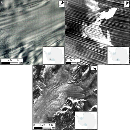
Subtle flow-parallel features are visible on satellite images of the surface of the Antarctic ice sheet. They are generally observed on its outlet glaciers, ice streams and ice shelves (Figure 1). Collectively, they are referred to as longitudinal surface structures (LSSs; Glasser & Gudmundsson, 2012) and are commonly subdivided into two categories. The term flow-stripe (alternatively ‘flow-band’, ‘streakline’ or ‘flow-line’) is usually retained for features which occur on top of fast-flowing ice streams of Antarctica (Figure 1(A)) and that continue onto ice shelves (Figure 1(B)), sustaining themselves for hundreds of kilometres (Crabtree & Doake, 1980; Merry & Whillans, 1993; Swithinbank, Brunt, & Sievers, 1988). Alternatively, the term foliation is usually applied to features which are found on the surface of glaciers (Figure 1(C)), with numerous examples occurring worldwide (Hambrey, 1975; Hooke & Hudleston, 1978; Jennings, Hambrey, & Glasser, 2014). A key distinguishing feature between the two terms is that foliations are the surface expression of a three-dimensional structure, caused by deformation and recrystallisation of the ice (Hambrey & Glasser, 2003), whereas flow-stripes may represent variations in surface reflectance of the ice which are non-topographic (Hulbe & Whillans, 1997). However, where the three-dimensional nature of LSSs visible on satellite images has been demonstrated in Antarctica (i.e. in bare ice areas), they too have been classified as foliations (e.g. Hambrey & Dowdeswell, 1994; Reynolds & Hambrey, 1988).

Figure 1. Examples of LSSs in different glaciological settings. (A) Landsat ETM+ image of flow-stripes on the surface of MacAyeal Ice Stream. (B) MODIS image of flow-stripes on the Ross Ice Shelf. (C) RADARSAT image of foliations on Erskine Glacier, Antarctic Peninsula.

As LSSs align themselves parallel with flow direction, and have a long residence time on the ice surface (Casassa & Whillans, 1994), relict features have been used in Antarctica to infer ice sheet history. On ice shelves, where their orientation or position deviates from current flow conditions, they have been used to reconstruct palaeo-flow configurations (e.g. Fahnestock, Scambos, Bindschadler, & Kvaran, 2000; Wuite & Jezek, 2009). LSSs found in the ice sheet interior have also been used to demonstrate switching ice stream flow direction and tributary configuration (Conway et al., 2002; Joughin et al., 1999). Additionally, flow-stripes found on the Bugenstock Ice Rise have been used to support evidence for flow direction change in the Weddell Sea sector of West Antarctica (Siegert, Ross, Corr, Kingslake, & Hindmarsh, 2013). Elsewhere, the configuration of LSSs across Antarctica suggests that the configuration of the ice sheet has remained unchanged for several thousand years (Glasser, Jennings, Hambrey, & Hubbard, 2014). However, whilst LSSs can be used as useful records of flow direction, their formation is not fully understood.

Multiple hypotheses have been proposed for the formation of LSSs (see Glasser & Gudmundsson, 2012, for a review). A leading hypothesis for the formation of flow-stripes sees them as the transmission of basal bumps in the bed to the ice surface, where the rate of basal sliding is high compared to internal deformation (Gudmundsson, Raymond, & Bindschadler, 1998). Additionally, it has been suggested that the basal bump which produces flow-stripes, under the right conditions, could be a subglacial bedform (Schoof, 2002). A further relationship between LSSs and subglacial bedforms is proposed within the groove-ploughing hypothesis for the formation of mega-scale glaciation lineations (Clark, Tulaczyk, Stokes, & Canals, 2003), whereby topographic undulations on the ice surface (foliations) might prolong the attenuation of basal keels ploughing into the underlying till. Under these hypotheses, LSSs may be able to inform us about the nature of the ice-bed interface. Conversely, foliations are hypothesised to form when pre-existing inhomogeneities in the ice (i.e. crevassing, stratification) are deformed and stretched down ice flow (Hambrey, 1977), occurring where ice flow is laterally compressive and longitudinally extensional (Glasser & Scambos, 2008; Hooke & Huddleston, 1978). LSSs also form as the consequence of shear between converging tributaries (Glasser & Gudmundsson, 2012). These models view LSSs as a product of cumulative ice strain (Hambrey & Lawson, 2000, p. 70), as opposed to a response to the properties of the bed.

The numerous examples of LSSs, and the diverse array of glaciological settings, mean that Antarctica is the ideal place to examine their characteristics and test the above models. Previous mapping has focused upon individual ice stream systems or ice shelves (e.g. Braun, Humbert, & Moll, 2009; Glasser et al., 2009, 2011; Holt, Glasser, & Quincey, 2013; Holt, Glasser, Quincey, & Siegfried, 2013; Reynolds & Hambrey, 1988). Here, our aim is to document LSSs across the entire Antarctic continent. Similar work has focussed on the utility of LSSs for reconstructing ice sheet history, focussing on individual ice streams (Glasser et al., 2014). However, the aim of our mapping is to shed light on how these enigmatic features might form. It is hoped that future morphometric analysis, combined with the geographic information system (GIS) databases detailing the glaciological characteristics of Antarctica (e.g. Fretwell et al., 2013; Rignot, Mouginot, & Scheuchl, 2011), will provide us with insights into the genesis of these features, in a similar manner to that which has been conducted upon subglacial bedforms (e.g. Spagnolo et al., 2014). Here, we document and present our mapping of LSSs visible on satellite imagery across the entire Antarctic continent.

2. Methods

2.1. Data and software

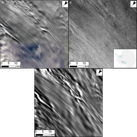
Mapping was conducted through manual on-screen digitisation at multiple scales in ESRI ArcMap 10. Cloud-free Landsat Enhanced Thematic Mapper Plus (ETM+) pan sharpened images of the Antarctic ice sheet are freely available for the region of Antarctica north of 82.5°S, and possess a horizontal pixel resolution of 15 m (http://lima.usgs.gov/). Multiple band combinations were used in this study. RADARSAT Antarctic Mapping Mission-2 synthetic aperture radar (SAR) images have a slightly lower resolution, 25 m, but are freely available for the entire continent (http://bprc.osu.edu/rsl/radarsat/data/). In some localities, the SAR waves likely penetrate the upper firn layers of the surface to depths of approximately 10–20 m (Ng & King, 2013). Additional reference was made to the MODIS Mosaic of Antarctica (http://nsidc.org/data/nsidc-0280.html). The multiple illumination angles composited into the mosaic allow for greater identification of subtle features, such as LSSs. However, MODIS images have lower spatial resolution (250 m), meaning that smaller features, typically found on valley glaciers, are unidentifiable on the images. Additionally, the oblique look angle of the MODIS satellite precludes mapping in valleys, as imagery is often obscured by valley walls. In many places across Antarctica, the number, distribution and alignment of identifiable features are indistinguishable between the three different sources of imagery, despite varying sensor properties and image resolution (e.g. Figure 2).

Figure 2. Comparison of the three sources of data used for mapping. Images of Ice Stream D, ice flow is from the top left of the image to bottom right. (A) Landsat ETM+ image (15 m resolution). (B) RADARSAT SAR image (25 m resolution). (C) MODIS mosaic image (125 m resolution). Features in this area are possibly clearest upon the MODIS imagery. However, there is a high level of agreement between all the images.

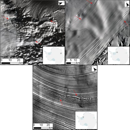
The subtlety of flow-stripes and foliations makes their identification problematic. Topographic LSSs on the Amery Ice Shelf have been shown to be only 1–2 m high, with a spacing of around 1 km (Hambrey & Dowdeswell, 1994; Raup, Scambos, & Haran, 2005). Adaptive contrast stretching (i.e. using local image statistics) was utilised in order to enhance the satellite images. LSSs were mapped along their perceived crest, the point of highest reflection or backscatter values. Often, features were interrupted by crevassing or by other surface features, only to reappear downstream (Figure 3). On ice shelves, this included disruption by features which have been interpreted to be the surface manifestation of subglacial channels (Le Broq et al., 2013; Figure 3(C)). Occasionally, a feature would fade out as it was traced downstream. Frequently, a second feature may reappear aligned with the original downstream, giving the impression of LSSs fading in and out of focus. As it would introduce ambiguity into our mapping, features were not joined across such interruptions. Whilst the higher resolution data sets (Landsat and RADARSAT) were preferred for mapping, all three sources were used to increase the likelihood of identifying features. Our map is genesis-blind, labelling features as only LSSs, rather than classifying into separate groups.

Figure 3. Examples of disrupted LSSs. Disruptions labelled with arrows. (A) Landsat image of crevassing disrupting LSSs as ice flows from Lepekhin Glacier towards the top right of the image onto the Amery Ice Shelf. (B) Landsat image of larger surface topography (transverse waves) interrupting LSSs on Recovery Glacier. (C) MODIS image of an ice shelf surface channel emanating from Slessor Glacier, disrupting LSSs on the Filchner Ice Shelf (formation discussed in Le Broq et al. (2013)).

The Main Map was produced in ArcGIS 10.1 and then imported into Inkscape v0.48. It comprises 42,311 polylines, representing either entire or portions of LSSs. The background for the map is a semi-transparent hillshade of the Radarsat Antarctic Mapping Project (RAMP) digital elevation model (DEM) v.2, underlain by the elevation model itself (http://nsidc.org/data/nsidc-0082.html). The grounding line position, where ice flows into the ocean and begins to float (Schoof, 2007), is also included on the map, in order to differentiate between grounded ice and ice shelves. This was also obtained from the RAMP (http://nsidc.org/data/nsidc-0082.html). The map is projected in WGS 1984 Antarctic Polar Stereographic. In order to highlight our mapping in key regions of the ice sheet, a series of three larger scale maps are also provided.

2.2. Accuracy and completeness of mapping

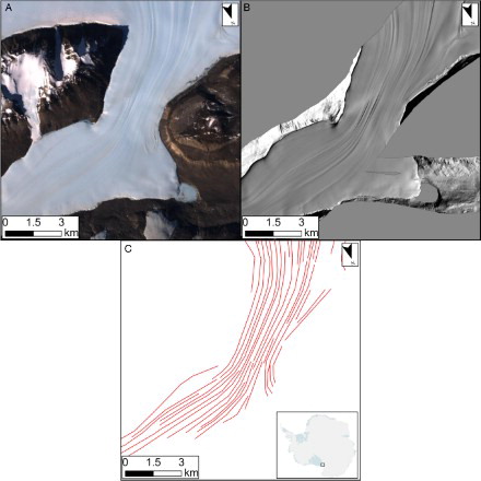
As our map covers the whole continent of Antarctica, ground-truthing of our mapping would be inconceivable. Even so, the subtlety of LSSs may preclude their identification in the field. An alternative is to compare the satellite data in which we perceive a mappable relief to high-resolution elevation models of relief. Figure 4 shows a comparison between Landsat data and a 2 m LiDAR-derived DEM of Taylor glacier (downloaded from http://nsidc.org/data/antarctic_dem.html). As Figure 4 demonstrates, there is good agreement between the two sources of data. This provides us with some confidence that the satellite images are representative of the glacier surface at an appropriate scale for identifying LSSs. However, to our knowledge, this is the only freely available high-resolution DEM covering Antarctica which contains LSSs. Although our mapping is the result of multiple passes of interpretation and from three sources of data, the large scale of the task may mean that some individual features may be missing from the final map. Additionally, subtle features that were undetected here may require more sensitive satellite instruments to detect.

Figure 4. Visual comparison between a Landsat image (A), a hillshaded high-resolution (2 m) LiDAR DEM (B) and mapping (C) of LSSs on Taylor Glacier. Whilst identification is easier upon high-resolution elevation models, no new features were identified upon the higher resolution model.

3. Results

3.1. The length of LSSs

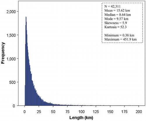
The length and persistence of LSSs are facets that any formation model must address (Gudmundsson et al., 1998; Merry & Whillans, 1993). Figure 5 is a histogram of the length of all mapped polylines. The sum of our length measurements totals over 650,000 km, roughly 16 times around the equator. The longest single traceable feature occurs on the Ronne Ice Shelf, and is 450 km in length. However, the distribution is heavily positively skewed (Figure 5), with the majority of measurements (80%) falling below 100 km. The histogram is unimodal, and therefore does not suggest separate morphometric populations. The distribution roughly approximates a log-normal or exponential function. The histogram is strongly peaked, with a modal bin of 10 km. LSSs are generally longer over ice shelves as opposed to on the surface of ice streams or glaciers. This is at least partially a consequence of other surface features interrupting our ability to trace LSSs (e.g. Merry & Whillans, 1993; Figure 3(B)). Overall, whilst exceptionally long LSSs occur, many much smaller features can also be noted. This is perhaps partially a consequence of our mapping technique, as we chose not to interpolate between possible disruptions in LSSs (e.g. Figure 3). However, the median length of a polyline is still above 8.6 km (Figure 5), highlighting that they persist for long distances on the surface of the ice sheet.

Figure 5. Histogram and descriptive statistics of LSS length. Bin width is 500 m. Note the strong positive skew of the distribution.

3.2. Spatial distribution

The accompanying map shows that LSSs are concentrated into the ice streams and outlet glaciers of the Antarctic Ice Sheet, and produce an arborescent pattern. The majority of LSSs therefore correspond to fast-flowing areas of the ice sheet (Figure 6). Most occur where ice is flowing above 50 m/a, and nearly all features were recorded in regions where ice flows above 20 m/a. However, notable exceptions to this do occur; these are labelled on Figure 6. LSSs are not limited to just the main channels of ice streams and outlet glaciers, as they can occur kilometers upflow from this, into the onset zones of fast flow (Figure 7). Mapped features also appear to be regularly spaced (Figure 8), especially once they have converged into a channel. However, this assertion awaits further morphometric analysis.

Figure 6. The correspondence between LSSs and ice velocity. Velocity data from Rignot et al. (2011) (http://nsidc.org/data/nsidc-0484.html). Areas where structures occur on ice flowing less than 20 m/a are labelled: (S) Siple Ice Stream (Conway et al., 2002), (K) Kamb Ice Stream (Catania, Hulbe, Conway, Scambos, & Raymond, 2012), (B) The Bugenstock Ice Rise (Siegert et al., 2013).

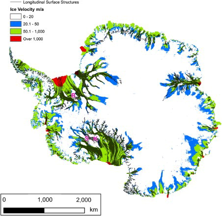
Figure 7. LSSs occurring in onset zones. Images from MODIS, velocity data from Rignot et al. (2011). (A) Subtle features at the onset to Lambert Glacier. (B) Onset zones of Whillans and Kamb Ice Streams.

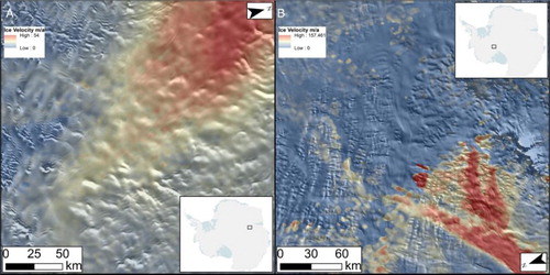
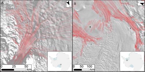
Figure 8. Examples of regular spacing of LSSs. Background is a semi-transparent MODIS image. (A) Mapped LSSs of Byrd Glacier. Note how features become evenly spaced as they converge into the main trunk of the glacier. (B) Regularly spaced flow-stripes of the Institute Ice Stream (I), Bugenstock Ice Rise (B) and Foundation Ice Stream (F).

4. Conclusions

Our mapping reveals the distribution and occurrence of LSSs across the Antarctic ice sheet. Landsat and RADARSAT images agree with high-resolution DEMs where available, suggesting that the satellite images are of an appropriate resolution for mapping these features. However, additional high-resolution data sets would provide more information on this issue and allow for a further level of morphometric analysis. Many longitudinal surface features are exceptionally long, but many shorter features also exist. The distribution of LSSs across Antarctica conforms to the arborescent pattern of ice flow, with features generally starting at onset zones to fast flow and converging into channels where their spacing appears to be regular. The map presented here will provide the basis for further research into LSSs on the Antarctic Ice Sheet.

5. Software

Mapping and data manipulation were conducted in ESRI ArcGIS 10.1. Further figure production was conducted in Inkscape v.0.48.

Acknowledgements

Cartography is from www.dvdmaps.co.uk. We would also like to thank M. J. Hambrey, T. Holt and H. Apps for their reviews which improved the original manuscript and map.

Funding

J. C. E. would like to thank Chris and Kathy Denison for funding his Ph.D., and acknowledges additional support from the L. R. Moore, University of Sheffield Alumni Scholarship.

References

- Braun, M., Humbert, A., & Moll, A. (2009). Changes of Wilkins Ice Shelf over the past 15 years and inferences on its stability. The Cryosphere, 3, 41–56. doi: 10.5194/tc-3-41-2009
- Casassa, G., & Whillans, I. M. (1994). Decay of surface topography on the Rose Ice Shelf, Antarctica. Annals of Glaciology, 20, 249–253. doi: 10.3189/172756494794587500
- Catania, G., Hulbe, C., Conway, H., Scambos, T. A., & Raymond, C. F. (2012). Variability in the mass flux of the Ross ice streams, West Antarctica, over the last millennium. Journal of Glaciology, 58, 741–752. doi: 10.3189/2012JoG11J219
- Clark, C. D., Tulaczyk, S. M., Stokes, C. R., & Canals, M. (2003). A groove-ploughing theory for the production of mega-scale glacial lineations, and implications for ice-stream mechanics. Journal of Glaciology, 49, 240–256. doi: 10.3189/172756503781830719
- Conway, H., Catania, G., Raymond, C. F., Gades, A. M., Scambos, T. A., & Engelhardt, H. (2002). Switch of flow direction in an Antarctic ice stream. Nature, 419, 465–467. doi: 10.1038/nature01081
- Crabtree, R. D., & Doake, C. S. M. (1980). Flow lines on Antarctic ice shelves. Polar Record, 20, 31–37. doi: 10.1017/S0032247400002898
- Fahnestock, M., Scambos, T., Bindschadler, R., & Kvaran, G. (2000). A millennium of variable ice flow recorded by the Ross Ice Shelf, Antarctica. Journal of Glaciology, 46, 652–664. doi: 10.3189/172756500781832693
- Fretwell, P., Pritchard, H. D., Vaughan, D. G., Bamber, J. L., Barrand, N. E., Bell, R., … Siegert, M. J. (2013). Bedmap2: Improved ice bed, surface and thickness datasets for Antarctica. The Cryosphere, 7, 375–393. doi: 10.5194/tc-7-375-2013
- Glasser, N. F., & Gudmundsson, G. H. (2012). Longitudinal surface structures (flowstripes) on Antarctic glaciers. The Cryosphere, 6, 383–391. doi: 10.5194/tc-6-383-2012
- Glasser, N. F., Jennings, S. J. A., Hambrey, M. J., & Hubbard, B. (2014). Are longitudinal ice-surface structures on the Antarctic ice sheet indicators of long-term ice-flow configuration? Earth Surface Dynamics Discussions, 2, 911–933. doi: 10.5194/esurfd-2-911-2014
- Glasser, N. F., Kulessa, B., Luckman, A., Jansen, D., King, E. C., Sammonds, P. R., … Jezek, K. C. (2009). Surface structure and stability of the Larsen C Ice Shelf, Antarctic Peninsula. Journal of Glaciology, 55, 400–410. doi: 10.3189/002214309788816597
- Glasser, N. F., & Scambos, T. A. (2008). A structural glaciological analysis of the 2002 Larsen B ice-shelf collapse. Journal of Glaciology, 54, 3–16. doi: 10.3189/002214308784409017
- Glasser, N. F., Scambos, T. A., Bohlander, J., Truffer, M., Petit, E., & Davies, B. J. (2011). From ice-shelf tributary to tidewater glacier: Continued rapid recession, acceleration and thinning of Röhss Glacier following the 1995 collapse of the Prince Gustav Ice Shelf, Antarctic Peninsula. Journal of Glaciology, 57, 397–406. doi: 10.3189/002214311796905578
- Gudmundsson, G. H., Raymond, C. F., & Bindschadler, R. (1998). The origin and longevity of flow-stripes on Antarctic ice streams. Annals of Glaciology, 27, 145–152.
- Hambrey, M. J. (1975). The origin of foliation in glaciers: Evidence from some Norwegian examples. Journal of Glaciology, 14, 181–185.
- Hambrey, M. J. (1977). Foliation, minor folds and strain in glacier ice. Tectonophysics, 39, 397–416. doi: 10.1016/0040-1951(77)90106-8
- Hambrey, M. J., & Dowdeswell, J. A. (1994). Flow regime of the Lambery Glacier-Amery Ice Shelf system, Antarctica: Structural evidence from Landsat imagery. Annals of Glaciology, 20, 401–406. doi: 10.3189/172756494794586943
- Hambrey, M. J., & Glasser, N. F. (2003). The role of folding and foliation development in the genesis of medial moraines: Examples from Svalbard glaciers. The Journal of Geology, 111, 471–485. doi: 10.1086/375281
- Hambrey, M. J., & Lawson, W. J. (2000). Structural styles and deformation fields in glaciers: A review. In A. J. Maltman, B. Hubbard, & M. J. Hambrey (Eds.), Deformation of glacial materials (Vol. 176, pp. 59–83). London: Geological Society (Special Publications).
- Holt, T. O., Glasser, N. F., & Quincey, D. J. (2013). The structural glaciology of southwest Antarctic Peninsula Ice Shelves (ca. 2010). Journal of Maps, 9, 523–531. doi: 10.1080/17445647.2013.822836
- Holt, T. O., Glasser, N. F., Quincey, D. J., & Siegfried, M. R. (2013). Speedup and fracturing of George VI Ice Shelf, Antarctic Peninsula. The Cryosphere, 7, 797–816. doi: 10.5194/tc-7-797-2013
- Hooke, R. Le B., & Hudleston, P. J. (1978). Origin of foliation in glaciers. Journal of Glaciology, 20, 285–299.
- Hulbe, C. L., & Whillans, I. M. (1997). Weak bands within Ice Stream B, West Antarctica. Journal of Glaciology, 43, 377–386.
- Jennings, S. J., Hambrey, M. J., & Glasser, N. F. (2014). Ice flow-unit influence on glacier structure, debris entrainment and transport. Earth Surface Processes and Landforms, 39, 1279–1292. doi: 10.1002/esp.3521
- Joughin, I., Gray, L., Bindschadler, R., Price, S., Morse, D., Hulbe, C., … Werner, C. (1999). Tributaries of West Antarctic ice streams revealed by RADARSAT interferometry. Science, 286, 283–286. doi: 10.1126/science.286.5438.283
- Le Broq, A. M., Ross, N., Griggs, J. A., Bingham, R. G., Corr, H. F., Ferraccioli, F., … Siegert, M. J. (2013). Evidence from ice shelves for channelized meltwater flow beneath the Antarctic Ice sheet. Nature Geoscience, 6, 945–948. doi: 10.1038/ngeo1977
- Merry, C. J., & Whillans, I. M. (1993). Ice-flow features on Ice Stream B, Antarctica, revealed by SPOT HRV imagery. Journal of Glaciology, 39, 515–527.
- Ng, F., & King, E. C. (2013). Formation of RADARSAT backscatter feature and undulating firn stratigraphy at an ice-stream margin. Annals of Glaciology, 54, 90–96. doi: 10.3189/2013AoG64A202
- Raup, B. H., Scambos, T. A., & Haran, T. (2005). Topography of streaklines on an Antarctic Ice Shelf from photoclinometry applied to a single advanced land imager (ALI) image. IEEE Transactions on Geoscience and Remote Sensing, IEEE Transactions on, 43, 736–742. doi: 10.1109/TGRS.2005.843953
- Reynolds, J. M., & Hambrey, M. J. (1988). The structural glaciology of George VI Ice Shelf, Antarctic Peninsula. British Antarctic Survey B, 79, 79–85.
- Rignot, E., Mouginot, J., & Scheuchl, B. (2011). Ice flow of the Antarctic ice sheet. Science, 333, 1427–1430. doi: 10.1126/science.1208336
- Schoof, C. (2002). Basal perturbations under ice streams: Form drag and surface expression. Journal of Glaciology, 48, 407–416. doi: 10.3189/172756502781831269
- Schoof, C. (2007). Ice sheet grounding line dynamics: Steady states, stability, and hysteresis. Journal of Geophysical Research: Earth Surface (2003–2012), 112(F3). doi:10.1029/2006JF000664
- Siegert, M., Ross, N., Corr, H., Kingslake, J., & Hindmarsh, R. (2013). Late Holocene ice-flow reconfiguration in the Weddell Sea sector of West Antarctica. Quaternary Science Reviews, 78, 98–107. doi: 10.1016/j.quascirev.2013.08.003
- Spagnolo, M., Clark, C. D., Ely, J. C., Stokes, C. R., Anderson, J. B., Andreassen, K., … King, E. C. (2014). Size, shape and spatial arrangement of mega-scale glacial lineations from a large and diverse dataset. Earth Surface Processes and Landforms, 39, 1432–1448.
- Swithinbank, C., Brunt, K., & Sievers, J. (1988). A glaciological map of Filchner-Ronne Ice Shelf, Antarctica. Annals of Glaciology, 11, 150–155.
- Wuite, J., & Jezek, K. C. (2009). Evidence of past fluctuations on Stancomb-Wills Ice Tongue, Antarctica, preserved by relict flow-stripes. Journal of Glaciology, 55, 239–244. doi: 10.3189/002214309788608732