Average monthly and annual climate maps for Bolivia

Abstract

This study presents monthly and annual climate maps for relevant hydroclimatic variables in Bolivia. We used the most complete network of precipitation and temperature stations available in Bolivia, which passed a careful quality control and temporal homogenization procedure. Monthly average maps at the spatial resolution of 1 km were modeled by means of a regression-based approach using topographic and geographic variables as predictors. The monthly average maximum and minimum temperatures, precipitation and potential exoatmospheric solar radiation under clear sky conditions are used to estimate the monthly average atmospheric evaporative demand by means of the Hargreaves model. Finally, the average water balance is estimated on a monthly and annual scale for each 1 km cell by means of the difference between precipitation and atmospheric evaporative demand. The digital layers used to create the maps are available in the digital repository of the Spanish National Research Council.

Keywords:

• precipitation
• temperature
• atmospheric water demand
• regression-based interpolation
• water balance
• Bolivia

1. Introduction

Climate maps are essential tools for land planning, crop and water management. This is especially critical in countries whose economic activities are highly dependent on climate variability (agriculture, livestock, hydropower production, etc.). The development of methods for interpolating local data from meteorological stations has allowed accurate maps of climate variables with high spatial resolution to be produced (Daly, Gibson, Taylor, Johnson, & Pasteris, 2002; Katsafados, Kalogirou, Papadopoulos, & Korres, 2012; Marsico, Caldara, Capolongo, & Pennetta, 2007; Ninyerola, Pons, & Roure, 2000). There are some climatology maps covering the entire Earth (Hijmans, Cameron, Parra, Jones, & Jarvis, 2005; New, Lister, Hulme, & Makin, 2002), but large-scale approaches commonly have problems related to the number of stations used and the fact that models used may not capture the variability of the climate conditions at the local scale. Moreover, to obtain accurate maps of climate variables, it is essential to guarantee high quality of the data inputs, and validation of the obtained results using independent data (Vicente Serrano, Saz, & Cuadrat, 2003).

Bolivia is expected to be one of the most affected countries by continental reductions in water supplies as a consequence of climate change (Winters, 2012). This underscores the need to employ available climate information for better preparedness and mitigation. Bolivia has very high climatic and environmental diversity as a consequence of marked topographic gradients and diverse natural ecosystems. The north and east Amazonian regions are characterized by evergreen equatorial forests (Navarro & Fereira, 2004), but the western Bolivian Altiplano (highlands) is dominated by dry tropical forests and large cultivated areas. Geographic and topographic diversity, and the influence of various atmospheric circulation mechanisms (Seiler, Hutjes, & Kabat, 2013) make the Bolivian climate highly complex over space and time (Escurra, Vazquez, Cestti, De Nys, & Srinivasan, 2014; Garcia, Raesb, Jacobsenc, & Micheld, 2007).

An indication of the importance of water availability in the region is that 50% of the active population of the Bolivian Altiplano is engaged in farming, with agricultural production of bitter potato and quinoa being major economic outputs and export commodities. Over a large part of the Altiplano the rainfall during the agricultural season is less than half of the atmospheric water demand (Vacher & Imaña, 1987), which reinforces negative agricultural impacts when a drought occurs (Vacher, 1998). In addition, Bolivian tropical dry forests are also highly sensitive to droughts, with secondary growth and net primary production being markedly reduced as a response to long-lasting droughts (Mendivelso, Camarero, Gutiérrez, & Zuidema, 2014; Seiler et al., 2014). For these reasons, an accurate evaluation of the climatology and the average water resources in the country must be the necessary first step toward providing climate services in the country.

In this study, we developed and validated digital monthly and annual climate maps for Bolivia at a spatial resolution of 1 km. National climate maps comprise not only precipitation and maximum and minimum air temperatures as input variables, but also atmospheric water demand and climatic water balance as derivative variables.

2. Methods

2.1. Climate data

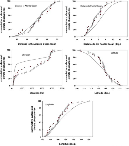
From 102 monthly total precipitation (P) series and 26 monthly maximum (T _max) and minimum (T _min) air temperature series from the National Meteorological & Hydrological Service of Bolivia, we selected those climate series having at least 25 years within the period 1950–2000. Both precipitation and air temperature series were tested for quality control and homogenization. The quality control procedure was based on the comparison of the rank of each data record with the average rank of the data recorded at adjacent stations (Vicente-Serrano et al., 2010). Relative homogeneity methods are commonly used to identify temporal homogeneity in climate series (Venema et al., 2012). For this purpose, we used relative homogeneity software, HOMER (Mestre et al., 2013), as a semi-automatic methodology that combines a fully automatic joint segmentation (Pickard et al., 2011) with a partly subjective pair-wise comparison (Caussinus & Mestre, 2004). HOMER takes advantage of the results of the benchmarking process conducted in the framework of the European Community COST ACTION ES0601 (http://www.homogenisation.org/): ‘Advances in homogenization methods of climate series: an integrated approach’, and includes some of the techniques recommended after an intercomparison study of the homogenization procedures (Venema et al., 2012). Checking for inhomogeneities in each P, T _max and T _min series was based on the analysis involving the nearby eight stations to each candidate station. The segmentation analysis was based on annual data, and used ratios for precipitation and temperature differences as a measure for comparisons. The method provides an estimation of break points in the time series relative to neighboring stations, and identifies high probabilities of the presence of inhomogeneities. Thus, if a break point was identified between a station and several of its neighboring stations for the same year, it was considered probable that there was inhomogeneity in the series. When a series presented an average ratio of one inhomogeneity every five years or larger, it was discarded and was not used for mapping. A total number of 68 precipitation series and 24 temperature series were selected to calculate the monthly averages at each station (Figure 1). The location of the available observatories covers different environmental conditions according to the distance to the oceans, elevation, latitude and longitude. Figure 2 shows the empirical cumulative distribution functions (ecdfs) for these variables corresponding to the location of the observatories and the entire surface of Bolivia. It shows how the observed range of these variables is satisfactorily covered by the available observatories, independently of the fit in the ecdfs. For example, although 60% of the territory in Bolivia is below 500 m and only 25% of the observatories are located below this elevation, there is very good representation of observatories over the whole range of the variable.

Figure 1. Elevation and meteorological stations available for precipitation and temperature in Bolivia (circles: selected stations; triangles: discarded stations).

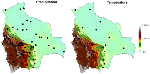
Figure 2. Empirical cumulative distribution functions (ecdfs) for the distance to the Atlantic and Pacific Oceans, Elevation, Latitude and Longitude corresponding to the location of the precipitation (circles) and temperature (triangles) observatories. Solid lines represent the ecdfs from 1 km gridded data sets for the entire Bolivia.

2.2. Climate mapping

Spatial interpolation of T _max, T _min and P was performed using regression-based techniques. A number of different interpolation procedures were used to obtain climate maps from punctual meteorological data: global, local and geostatistics techniques (Borrough & McDonnell, 1998). The most widely used procedures are global methods based on regression techniques. In these methods, different geographic and topographic factors that control the spatial distribution of climate are used as independent variables (Daly et al., 2002; Ninyerola et al., 2000), and dependence models are created between the climate data and independent variables. The value of a climate variable in unsampled points is obtained according to the following equation:where z is the predicted value of the climate variable at point x; b ₀   …  b_n are the regression coefficients and P ₁   … P_n are the values of the different independent variables at point x.

The main advantage of this technique is that climate maps are compiled not only from information from various weather stations, but also from auxiliary information that describes geographic and topographic variables; this approach improves the accuracy and spatial detail of the resulting maps. We used independent variables at a spatial resolution of 1 km. The independent variables were elevation, latitude, longitude and distance to the Atlantic and Pacific oceans. Elevation was obtained from the Global Multi-resolution Terrain Elevation Data 2010 (GMTED, 2010) digital elevation model (DEM) at a resolution of 7.5 arc-second (https://lta.cr.usgs.gov/GMTED2010), which was rescaled to 1 km of spatial resolution in a latitude–longitude projection with datum WGS-84. The distance to the Atlantic and Pacific oceans was obtained from the coastlines using the BUFFDIST module of the MiraMon geographic information system (GIS) (Pons, 2006). Low-pass filters with radii of 2.5, 5, 12.5 and 25 km were applied to elevation in order to measure the wider influence of this variable on climate. Nevertheless, these filtered variables were only included for modeling precipitation. For temperature, we only included elevation to avoid that inclusion of elevation with different low-pass filters that may cause the maximum temperature to be lower than the minimum temperature, given the different variables included in the model. Although some studies have also recommended the inclusion of the effect that topographic barriers may produce on climatic variables, for example, using the maximum height in a wedge of given aspect and radius (Agnew & Palutikof, 2000), we discarded its use since the strong topographic complexity in Bolivia can cause artificial boundaries between adjacent areas with no climatological meaning. The normality of each variable was tested using the Kolmogorov–Smirnov test, and natural logarithms were applied where necessary in order to fit a normal distribution more closely. Correlation between independent variables leads to problems with collinearity. To avoid this, we followed Hair, Anderson, Tatham, and Black (1998) and applied a forward stepwise procedure with ‘probability to enter’ set to 0.01 to retain only significant independent variables.

The disadvantage of using regression-based techniques to map climate data is that the results are inexact because the predicted value of the climatic variable z(x) does not coincide with the real data collected at weather stations; however, the error obtained at each point is known (residual) and we performed a procedure to correct it. The residuals (difference between the climatic variable measured at a weather station and that predicted by the model) were spatially interpolated using inverse distance weighting, and the resulting ‘residual maps’ were added to the regression maps, thus refining the results (Ninyerola et al., 2000).

2.3. Calculation of the atmospheric water demand

A number of different methods are used to calculate atmospheric evaporative demand (AED) (Allen, Pereira, Raes, & Smith, 1998). The Food and Agriculture Organization of the United Nations (FAO) have adopted the Penman–Monteith (PM) method (Allen et al., 1998) as the standard for computing AED from climate data including a reference surface resistance term based on standard crop (reference evapotranspiration – ETo). Nevertheless, the PM needs a large amount of data, as it requires values of solar radiation, wind speed and relative humidity, which are not available in Bolivia.

Several authors have proposed the empirical Hargreaves (HG) equation (Hargreaves & Samani, 1985) as the best alternative where data are scarce (Martínez-Cob, 2002; Vicente-Serrano et al., 2014; Xu & Singh, 2001). This method only requires information on T _max, T _min and extraterrestrial radiation (R _a). Because R _a can be calculated theoretically (Droogers & Allen, 2002), the only variables required in this method are observed air temperatures. Droogers and Allen (2002) modified the original HG equation by including a rainfall term, on the assumption that monthly P can represent relative levels of humidity and solar radiation. The ETo (mm day⁻¹) is calculated aswhere P is the monthly total precipitation in mm, R is the difference between the maximum and minimum temperatures (monthly averages; °C) and R _a is the extraterrestrial solar radiation (mm day⁻¹). R _a values are modeled from the DEM at a cell size of 1 km. For this purpose, we used an algorithm that considers the effects of terrain complexity (shadowing and reflection) and the daily solar position (Pons & Ninyerola, 2008). R _a is provided in MJ m⁻² day⁻¹, which is transformed to mm day⁻¹ (1 MJ m⁻² day⁻¹ = 0.408 mm day⁻¹). Vicente-Serrano, Lanjeri, and López-Moreno (2007) showed that this approach provides more accurate estimations of ETo than estimating R _a only according to the latitude and the day of the year.

We used the modified HG method to obtain monthly maps of ETo at a spatial resolution of 1 km using the grids of P, T _max and T _min obtained by means of regression-based interpolation and the R _a modeled by means of the DEM.

2.4. Calculation of the climatic water balance

We calculated a simple climatic water balance model by means of the difference between P and ETo, monthly and annually (Thornthwaite, 1948). This measure, although not considered the water runoff potential in each grid cell, can be considered as a measure of the average long-term water deficit or surplus, which is very useful as a measure of water stress and so can be used to obtain robust drought indices (Vicente-Serrano, Beguería, & López-Moreno, 2010).

2.5. Validation

In the absence of a sufficient number of observatories (68 precipitation and 24 temperature observatories for the whole country), the ‘jack-knifing’ method was adopted for validation, based on withholding, in turn, one station out of the network, estimating climate at each point according to the procedure explained in Section 2.2 from the remaining observatories and calculating the difference between the predicted and observed values for each withheld observatory (Phillips, Dolph, & Marks, 1992). This method has frequently been used in climatology (Daly, Neilson, & Phillips, 1994; Hofstra, Haylock, New, Jones, & Frei, 2008; Holdaway, 1996), particularly where a low number of cases are available for validation.

The performance of each map is assessed by means of different validation statistics. Combining the benefits of a range of statistical estimators can provide a more rigorous assessment of the model uncertainty. In this work we used three accuracy estimators, including bias, the mean absolute error (MAE) and the D Willmott's refined index of agreement (Willmott, Robeson, & Matsuura, 2012).

The bias is calculated as a measure of the differences in values between the observed (O) and model (P) data, and is given aswhere N is the sample size, O is the observed value and P is the model value at station i.

The MAE is calculated as the average of the absolute difference between observed and predicted data:

The refined D Willmott statistic is a measure of agreement/disagreement between the observed and modeled data, reflecting not only differences in their means, but also differences in their standard deviations. This coefficient is dimensionless as it is bounded between −1 (no agreement) and 1 (perfect agreement). According to Willmott et al. (2012), the D statistic is given as

when

and

when

3. Results

Table 1 shows the results for the regression model fit corresponding to the monthly P, T _max and T _min using as predictors the topographic and geographic variables indicated earlier. The fit is better for maximum and minimum temperatures than for precipitation in the majority of months. Minimum temperatures also show higher R² values than maximum temperature. There are no noticeable seasonal differences in the fit of the different models.

Table 1. Results of the monthly models to map precipitation, and maximum and minimum temperatures.

	R^2	Adjusted R^2	f	p
Precipitation
January	0.66	0.64	38.9	0.049
February	0.64	0.63	47.2	0.042
March	0.67	0.66	53.5	0.003
April	0.89	0.88	124.4	0
May	0.84	0.83	103.3	0.01
June	0.58	0.57	36.9	0.006
July	0.70	0.67	34.4	0
August	0.64	0.63	48	0.004
September	0.71	0.69	63.8	0.002
October	0.80	0.80	163.2	0
November	0.85	0.95	156.4	0
December	0.75	0.73	57.4	0.003
Maximum temperature
January	0.94	0.94	279.7	0
February	0.94	0.93	274.1	0
March	0.92	0.92	236.5	0
April	0.89	0.89	157.2	0
May	0.86	0.85	222.8	0.002
June	0.85	0.84	68.8	0.002
July	0.87	0.86	83.4	0.001
August	0.90	0.90	334.1	0
September	0.91	0.91	190.9	0
October	0.91	0.91	189.5	0
November	0.91	0.90	177.3	0
December	0.92	0.92	219.0	0
Minimum temperature
January	0.98	0.95	927.9	0
February	0.98	0.95	1757.4	0
March	0.98	0.98	1635.2	0
April	0.98	0.96	1590.6	0
May	0.96	0.96	420.9	0
June	0.91	0.91	192.0	0
July	0.90	0.90	168.7	0.001
August	0.91	0.90	120.5	0
September	0.93	0.93	150.7	0
October	0.94	0.94	543.4	0
November	0.95	0.94	673.6	0
December	0.97	0.96	1073.3	0

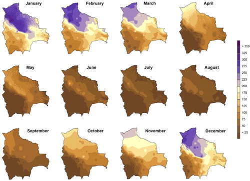
Figures 3–5 show the spatial distribution of T _max, T _min and P, respectively. Precipitation shows strong geographical gradients and noticeable seasonality. The humid season spans from November to March. Maximum precipitation is recorded in the north and northwest areas, which correspond to the Amazon basin and the slopes that separate this area from the elevated Altiplano. The Altiplano receives much less precipitation, which is concentrated in the summer period. Maximum and minimum temperatures also show seasonality and noticeable spatial differences, mainly controlled by relief.

Figure 3. Spatial distribution of monthly maximum temperature (°C) obtained from regression-based modeling and local interpolation of residuals.

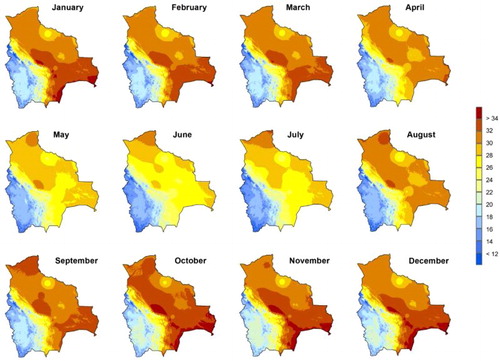
Figure 4. Spatial distribution of monthly minimum temperature (°C) obtained from regression-based modeling and local interpolation of residuals.

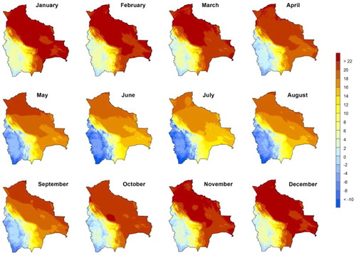
Figure 5. Spatial distribution of monthly precipitation (mm) obtained from regression-based modeling and local interpolation of residuals.

The agreement between observed and estimated values obtained by means of the jackknife approach is high (Figure 6, Table 2). The fit between observed and predicted data is higher for minimum temperature than for maximum temperature. Moreover, precipitation underestimation is observed at some meteorological stations. Bias and MAE values show a clear seasonal pattern, which is in agreement with precipitation and temperature seasonality. In general precipitation shows a negative bias, which means that predictions tend to underestimate observations, whereas minimum temperature tends to be overestimated. Annual MAE is 141.1 mm for precipitation and 1.5°C for maximum and 1.6°C for minimum temperatures. The D statistic, which allows comparison between months and variables, shows high values (D > 0.9 for precipitation between April and November). For temperature the D values are always higher than 0.84, which demonstrates good agreement between the magnitude and spatial distribution of observed and predicted values. Annual D is around 0.9 in the three modeled variables, which provides high confidence in the predicted values with respect to the observed range of these variables.

Figure 6. Relationship between observed and predicted monthly precipitation and temperature using the jackknife approach.

Table 2. Error/accuracy statistics for the monthly precipitation and temperature maps.

		J	F	M	A	M	J	J	A	S	O	N	D	Annual
MAE (mm)	Precip	25.169	23.990	22.708	11.463	8.346	7.073	5.456	6.382	8.784	11.872	15.337	23.241	141.154
	T max	1.537	1.453	1.469	1.600	1.528	1.615	1.626	1.548	1.587	1.676	1.714	1.664	1.532
	T min	0.913	0.920	0.995	1.394	1.968	2.281	2.366	2.309	1.999	1.655	1.495	1.195	1.624
MBE (mm)	Precip	−1.868	−1.848	−1.184	−0.046	−0.225	−0.010	0.129	−1.102	−0.665	−1.061	−1.175	0.794	−8.260
	T max	0.063	0.045	0.004	−0.072	−0.050	−0.021	−0.006	0.009	0.039	0.031	0.053	0.047	0.012
	T min	0.136	0.146	0.136	0.221	0.322	0.336	0.320	0.332	0.338	0.308	0.275	0.203	0.256
D	Precip	0.749	0.752	0.800	0.947	0.969	0.976	0.982	0.978	0.967	0.944	0.904	0.772	0.901
	T max	0.889	0.894	0.893	0.883	0.886	0.877	0.877	0.886	0.886	0.883	0.881	0.882	0.889
	T min	0.938	0.937	0.931	0.900	0.855	0.858	0.862	0.844	0.853	0.882	0.895	0.918	0.889

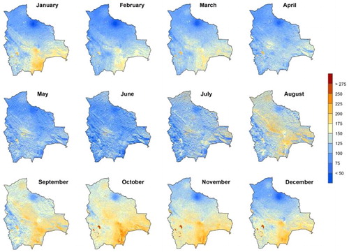
Figure 7 shows the spatial distribution of monthly ETo that exhibits strong spatial differences between neighboring areas as a consequence of the complex relief. The main contrast is recorded between southern and northern slopes during the cold season. In winter, the ETo is mainly controlled by the available radiation, whereas in summer the mean temperature and the daily temperature range play a major role in ETo rates, explaining the reason for the lower topographic control of ETo during summer.

Figure 7. Spatial distribution of monthly ETo (mm) obtained from maximum and minimum temperatures and the relief-based modeled solar radiation.

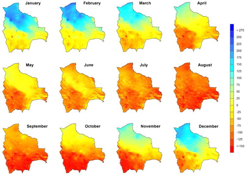
Figure 8 shows the spatial distribution of the climatic water balance (the difference between precipitation and ETo). The different plots show strong seasonal differences between the humid season (November–March), in which positive values are dominant, and the dry season (April–October), in which negative values are recorded, mainly in the Altiplano region.

Figure 8. Spatial distribution of monthly climatic water balance (mm) by means of the difference between precipitation and ETo.

Climate averages shown in the main Annual Climate Map for Bolivia (Main Map) stress the strong contrasts of climate in the country and the clear separation between the Amazonian basin (North) and the Altiplano (Southwest), the latter characterized by limiting climate conditions for the development of natural vegetation and agriculture (i.e. low precipitation, cold temperatures and negative water balances).

4. Conclusions

We have created monthly and annual precipitation and maximum and minimum temperature maps for Bolivia at a spatial resolution of 1 km using regression-based modeling, with topographic and geographic variables as independent variables. The different monthly climate maps have shown good agreement between observations and predictions with an agreement index (D) around 0.9. MAE for annual values is 141 mm for precipitation and around 1.5°C for both maximum and minimum temperatures. These errors can be considered low given the high precipitation and temperature ranges in the country (>2000 mm and >20°C, for precipitation and temperature, respectively).

We have also created climate maps for atmospheric water demand based on precipitation, temperature and the modeled exoatmospheric solar radiation derived from the topography. The differences in the atmospheric water demand across Bolivia are very important with approximately 1800–2000 mm year⁻¹. In the south and southeast areas, the atmospheric water demand is higher than 2000 mm year⁻¹. The variation in precipitation and atmospheric water demand shows that large areas of Bolivia have a strong annual water deficit (>1000 mm year⁻¹) and that humid areas are restricted to the northern part of the Amazonian basin and the transitional slopes to the Altiplano. The 1 km monthly and annual digital layers of precipitation, maximum and minimum temperatures, ETo and climatic water balance are available in ArcGIS ASCIIformat in the web repository of the Spanish National Research Council (CSIC) at https://digital.csic.es/handle/10261/103342.

Software

MiraMon v6.4 software was used for map modeling and generating the raster layers. Esri ArcGis 9.3 was used to produce the final maps.

Additional information

Funding

This work was supported by research projects I-COOP H₂O 2013CD0006: ‘Test multisectorial y actividades demostrativa sobre el potencial desarrollo de sistemas de monitorización de sequías en tiempo real en la región del oeste de Sudamérica’ financed by the Spanish National Research Council (CSIC), CGL2011-27574-CO2-02 financed by the Spanish Commission of Science and Technology and FEDER, and ‘LIFE12 ENV/ES/000536 Demonstration and validation of innovative methodology for regional climate change adaptation in the Mediterranean area (LIFE MEDACC)’ financed by the LIFE program of the European Commission. C. A-M received a postdoctoral fellowship# JCI-2011-10263. A. S-L is supported by the postdoctoral fellowship # JCI-2012-12508.

References

- Agnew, M. D., & Palutikof, J. P. (2000). GIS-based construction of base line climatologies for the Mediterranean using terrain variables. Climate Research, 14, 115–127. doi: 10.3354/cr014115
- Allen, R. G., Pereira, L. S., Raes, D., & Smith, M. (1998). Crop evapotranspiration: Guidelines for computing crop requirements, irrigation and drainage paper 56. Roma: FAO.
- Borrough, P. A., & McDonnell, R. A. (1998). Principles of geographical information systems. Oxford: Oxford University Press.
- Caussinus, H., & Mestre, O. (2004). Detection and correction of artificial shifts in climate series. Journal of the Royal Statistical Society: Series C (Applied Statistics), 53, 405–425. doi:10.1111/j.1467-9876.2004.05155.x
- Daly, C., Gibson, W. P., Taylor, G. H., Johnson, G. L., & Pasteris, P. (2002). A knowledge-based approach to the statistical mapping of climate. Climate Research, 22, 99–113. doi: 10.3354/cr022099
- Daly, C., Neilson, R. P., & Phillips, D. L. (1994). A statistical topographic model for mapping climatological precipitation over mountain terrain. Journal of Applied Meteorology, 33, 140–158. doi: 10.1175/1520-0450(1994)033<0140:ASTMFM>2.0.CO;2
- Droogers, P., & Allen, R. G. (2002). Estimating reference evapotranspiration under inaccurate data conditions. Irrigation and Drainage Systems, 16, 33–45. doi: 10.1023/A:1015508322413
- Escurra, J. J., Vazquez, V., Cestti, R., De Nys, E., & Srinivasan, R. (2014). Climate change impact on countrywide water balance in Bolivia. Regional Environmental Change, 14, 727–742. doi: 10.1007/s10113-013-0534-3
- Garcia, M., Raesb, D., Jacobsenc, S.-E., & Micheld, T. (2007). Agroclimatic constraints for rainfed agriculture in the Bolivian Altiplano. Journal of Arid Environments, 71, 109–121. doi: 10.1016/j.jaridenv.2007.02.005
- Hair, J. F., Anderson, R. E., Tatham, R. L., & Black, W. C. (1998). Multivariate data analysis. New York: Prentice Hall International. p. 799.
- Hargreaves, G. L., & Samani, Z. A. (1985). Reference crop evapotranspiration from temperature. Applied Engineering in Agriculture, 1, 96–99. doi: 10.13031/2013.26773
- Hijmans, R. J., Cameron, S. E., Parra, J. L., Jones, P. G., & Jarvis, A. (2005). Very high resolution interpolated climate surfaces for global land areas. International Journal of Climatology, 25, 1965–1978. doi: 10.1002/joc.1276
- Hofstra, N., Haylock, M., New, M., Jones, P., & Frei, C. (2008). The comparison of six methods for the interpolation of daily European climate data. Journal of Geophysical Research, 113, D21110. doi:10.1029/2008JD010100
- Holdaway, M. R. (1996). Spatial modeling and interpolation of monthly temperature using kriging. Climate Research, 6, 215–225. doi: 10.3354/cr006215
- Katsafados, P., Kalogirou, S., Papadopoulos, A., & Korres, G. (2012). Mapping long-term atmospheric variables over Greece. Journal of Maps, 8, 181–184. doi: 10.1080/17445647.2012.694273
- Marsico, A., Caldara, M., Capolongo, D., & Pennetta, L. (2007). Climatic characteristics of middle-southern Apulia (southern Italy). Journal of Maps, 3, 342–348. doi: 10.1080/jom.2007.9710849
- Martínez-Cob, A. (2002). Infraestimación de la evapotranspiración potencial con el método de Thornthwaite en climas semiáridos. In J. M. Cuadrat, S. M. Vicente, & M. A. Saz (Eds.), La Información Climática Como Herramienta de Gestión Ambiental (pp. 117–122). Zaragoza: Universidad de Zaragoza.
- Mendivelso, H. A., Camarero, J. J., Gutiérrez, E., & Zuidema, P. A. (2014). Time-dependent effects of climate and drought on tree growth in a Neotropical dry forest: Short-term tolerance vs. long-term sensitivity. Agricultural and Forest Meteorology, 188, 13–23. doi: 10.1016/j.agrformet.2013.12.010
- Mestre, O., Domonkos, P., Picard, F., Auer, I., Robin, S., Lebarbier, E., … Stepanek, P. (2013). Homer: A homogenization software – Methods and applications. IDOJÁRÁS. Quarterly Journal of the Hungarian Meteorological Service, 117, 47–67.
- Navarro, G., & Fereira, W. (2004). Zonas de vegetación potencial de Bolivia: una base para el análisis de vacíos de conservación. Revista Boliviana de Ecología, 15, 1–40.
- New, M., Lister, D., Hulme, M., & Makin, I. (2002). A high-resolution data set of surface climate over global land areas. Climate Research, 21, 1–25. doi: 10.3354/cr021001
- Ninyerola, M., Pons, X., & Roure, J. M. (2000). A methodological approach of climatological modelling of air temperature and precipitation through GIS techniques. International Journal of Climatology, 20, 1823–1841. doi: 10.1002/1097-0088(20001130)20:14<1823::AID-JOC566>3.0.CO;2-B
- Phillips, D. L., Dolph, J., & Marks, D. (1992). A comparison of geostatistical procedures for spatial analysis of precipitation in mountainous terrain. Agricultural and Forest Meteorology, 58, 119–141. doi: 10.1016/0168-1923(92)90114-J
- Picard, F., Lebarbier, E., Hoebeke, M., Rigaill, G., Thiam, B., & Robin, S. (2011). Joint segmentation, calling, and normalization of multiple CGH profiles. Biostatistics, 12(3), 413–428. doi:10.1093/biostatistics/kxq076
- Pons, X. (2006). Manual of miramon. Geographic Information System and Remote Sensing Software. Bellaterra: Centre de Recerca Ecol`ogica i Aplicacions Forestals (CREAF). Retrieved from http://www.creaf.uab.es/miramon
- Pons, X., & Ninyerola, M. (2008). Mapping a topographic global solar radiation model implemented in a GIS and refined with ground data. International Journal of Climatology, 28, 1821–1834. doi: 10.1002/joc.1676
- Seiler, C., Hutjes, R. W. A., & Kabat, P. (2013). Likely ranges of climate change in Bolivia. Journal of Applied Meteorology and Climatology, 52, 1303–1317. doi: 10.1175/JAMC-D-12-0224.1
- Seiler, C., Hutjes, R. W. A., Kruijt, B., Quispe, J., Añez, S., Arora, V. K., … Kabat, P. (2014). Modeling forest dynamics along climate gradients in Bolivia. Journal of Geophysical Research: Biogeosciences, 119, 758–775.
- Thornthwaite, C. W. (1948). An approach toward a rational classification of climate. Geographical Review, 38, 55–94. doi: 10.2307/210739
- Vacher, J. J. (1998). Responses of two main Andean crops, quinoa, Chenopodium quinoa Willd and papa amarga Solanum juzepczukii Buk. to drought on the Bolivian Altiplano: Significance of local adaptation. Agriculture, Ecosystems and Environment, 68, 99–108. doi: 10.1016/S0167-8809(97)00140-0
- Vacher, J. J., & Imaña, E. (1987). Los riesgos climaticos en el altiplano Boliviano. OMM-SENAMHI-ORSTOM, La Paz, Bolivia, 30.
- Venema, V. K. C., Mestre, O., Aguilar, E., Auer, I., Guijarro, J. A., Domonkos, P., … Brandsma, T. (2012). Benchmarking homogenization algorithms for monthly data. Climate of the Past, 8(1), 89–115. doi: 10.5194/cp-8-89-2012
- Vicente-Serrano, S. M., Azorin-Molina, C., Sanchez-Lorenzo, A., Revuelto, J., López-Moreno, J.I., González-Hidalgo, J.C., & Espejo, F. (2014). Reference evapotranspiration variability and trends in Spain, 1961–2011. Global and Planetary Change, 121, 26–40. doi: 10.1016/j.gloplacha.2014.06.005
- Vicente-Serrano, S. M., Beguería, S., López-Moreno, J.I., García-Vera, M.A., & Stepanek, P. (2010). A complete daily precipitation database for North-East Spain: reconstruction, quality control and homogeneity. International Journal of Climatology, 30, 1146–1163. doi: 10.1002/joc.1850
- Vicente-Serrano, S. M., Beguería, S., & López-Moreno, J.I. (2010). A Multi-scalar drought index sensitive to global warming: The Standardized Precipitation Evapotranspiration Index – SPEI. Journal of Climate, 23, 1696–1718. doi: 10.1175/2009JCLI2909.1
- Vicente-Serrano, S. M., Lanjeri, S., & López-Moreno, J. I. (2007). Comparison of different procedures to map reference evapotranspiration using geographical information systems and regression-based techniques. International Journal of Climatology, 27, 1103–1118. doi: 10.1002/joc.1460
- Vicente Serrano, S. M., Saz, M. A., & Cuadrat, J. M. (2003). Comparative analysis of interpolation methods in the middle Ebro valley (Spain): application to annual precipitation and temperature. Climate Research, 24, 161–180. doi: 10.3354/cr024161
- Willmott, C. J., Robeson, S. M., & Matsuura, K. (2012). A refined index of model performance. International Journal of Climatology, 32, 2088–2094. doi: 10.1002/joc.2419
- Winters, C. (2012). Impact of climate change on the poor in Bolivia. Global Majority E-Journal, 3, 33–43.
- Xu, C. Y., & Singh, V. P. (2001). Evaluation and generalization of temperature based methods for calculating evaporation. Hydrological Processes, 15, 305–319. doi: 10.1002/hyp.119