3D geological model of an overthrust napped structure. Hășmaș mountains, Eastern Carpathians, Romania

ABSTRACT

This work represents an improvement of the methodology applied in the geological study of a napped structure by approaching the fault system and the formations in a 3D volumetric space. From a geological point of view, the studied area contains two thrust nappes: the Hășmaș Nappe, which is a gravitational nappe and the Bukovinian Nappe, which is an overthrust nappe. By combining data obtained from field measurements with the bibliographic support, we performed an overview of the study area. The 3D geological model has been achieved by the interpretation and drawing of 54 geological cross sections based on preexisting geological maps and accumulated field knowledge, using GSI3D and Move3D software. By using the model, one can extract information about any point in the space occupied by it, allowing real-time visualization. Also the 3D model provides a means to accurately estimate the exact limits of the strata, giving their volumes and surfaces in the context of a possible natural reserve calculation.

KEYWORDS:

• 3D geological model
• overthrust nappes
• GSI3D
• move 3D
• Hășmaș mountains
• Eastern Carpathians
• Romania

1. Introduction

Geological maps represent the interpretation of faults and geological formations in structural arrangements at the land surface. Their correlation into the subsurface is achieved by constructing geological cross sections.

Many times the classical geological representation of an area (from maps and cross sections) are not enough to capture all the information a geologist may have in an area, because not all elements of the area are represented or interpreted in a regional context. Recently, because of technological and operational developments in 3D geologic – modeling, geologists are now able to transfer their experience and knowledge in a volumetric space, which facilitates the exchange of information between all types of specialists.

Constructing such a 3D geological model arose from the need to visualize the spatial arrangement of geological formations, defined by the axes x, y and z and their depth and thickness, thus improving their study and interpretation such as some parts in the Tulgheș-Hășmaș-Ciuc syncline.

The Tulgheș-Hășmaș-Ciuc syncline belongs to the high median area within the Central Group of the Eastern Carpathians, and encompasses a mountain area of approximately 3420 km² known as the Hășmaș Mountains, with altitudes between 800 and 1792 m (Hășmașul Mare).

2. Geological settings

Geologically, the Tulgheș-Hășmaș-Ciuc syncline corresponds to the Hășmaș syncline, which together with the Rarău syncline form the External Marginal Syncline.

The studied area is marked by the presence of two thrust nappes: the Hășmaș Nappe, which is a gravitational nappe and the Bukovinian Nappe, which is an overthrust nappe (Figure 1).

2.1. Stratigraphy

2.1.1. Bedrock

The only part of the Precambrian basement rock in the study area is the Hășmaș Granitoid, which is part of a larger group known as Bretila-Rarău.

Precambrian – Hășmaș Granitoid: Massive rocks without any significant stratification consisting of granodiorite and gneiss diorite.

2.1.2. Bukovinian nappe

Here, the Bukovinian nappe encompasses formations with ages between the Upper Paleozoic and Barremian-Albian.

Upper Paleozoic – Hășmaș Breccia: This formation has a high prevalence on the west flank of the Hășmaș Syncline and contains large clasts welded in a heterogeneous cement.

Lower induan – conglomerate and sandstone: The Lower induan interval from the Bukovinian nappe contains white, yellow or reddish conglomerate and sandstone, and has a thickness of approximately 30 m (Grasu, Miclăuș, Brânzilă, & Baciu, 2012).

Induan-Olenekian – dolomite: The Induan-Olenekian formation has the largest aerial extent of all Triassic bedrock in the Bukovinian nappe. These rocks are massive, with faint stratification, a yellowish-white or red color, with a coarse aspect.

Ladinian – limestone: This package of rocks has a variable thickness, generally from 10 to 60 m and even, to a maximum of 180 m in some areas. It has a yellowish-white or grey color, and high carbonates content, which is characteristic of pure limestone.

Upper Triassic – limestone and dolomite: The dolomite has a thickness between 20 and 100 m, has a pink, reddish or yellowish-white color, and is crossed by calcite.

The limestone has a red or whitish-yellow color and it interpolates with dolomites which demonstrates a dolomitization process (Grasu et al., 2012).

Middle Jurassic – sandstone-limestone: The Middle Jurassic bedrock is divided into three units:

1. A lower unit having a thickness of 90 m and a macroscopic appearance of limestone.

2. A middle unit with rock having a high hardness, a color very similar to the lower unit, and which consists exclusively of spongolitic limestone.

3. An upper unit that consists of limestone to sandstone with petrified plant remains (Grasu, Turculeţ, Catana, & Niţă, 1995).

Albian-Barremian – the Wildflysch formation: Săndulescu (1975) was the first to separate this formation into three units: a lower unit containing jasper, and two alternating units, one including a shaly matrix with different types of intraclasts and another that has a flysch-type character, consisting of mudstone, sandstone to laminated mudstone and limestone to sandstone.

2.1.3. Hășmaș nappe

The Hășmaș nappe encompasses formations with ages between the Kimmeridgian and Tithonian-Neocomian.

Lower Induan – limestone: This type of red, compact limestone is found exclusively in the form of blocks incorporated in the wildflysch formation.

Kimmeridgian – limestone: This formation has a thickness of 30–40 m and it is divided into two units: a lower red limestone unit that has a thickness of 6 m, and includes an upper greenish-grey limestone having a thickness of approximately 25 m.

Tithonian – lower Cretacic limestone: This yellowish-white to gray limestone is divided into the ‘Stramberg’ limestone (Tithonian age), which has an approximately 200 m thickness, and neocomian limestone that is approximately 100 m thick.

2.2. Tectonics

The most important deformation of the Bukovinian nappe occurred after deposition of the Wildflysch. Other, older deformations are situated between the Hettangian and Aalenian rocks, just below the deposition of the Berriasian formation and between the Hauterivian and Barremian.

The overthrust of the Bukovinian nappe is very large, but the nappe's internal structure is fairly simple, with normal and scarcely ever overturned folds, due to the stiffness of the crystalline schist, which composes a large part of the nappe.

The Hășmaș nappe has been deformed twice. The first phase occurred between the Kimmeridgian and Tithonian periods, and the second one between the Berriasian and Barremian periods.

Between the Barremian and Albian periods the nappe was subject to a gravitational slide, which cannot be considered an actual deformation stage. The area of its origin is 60–70 km to the west. Its movement, toward the east, was very slow, stopping near the basin's axis, where the wildflysch formation was deposited.

In this area, the internal architecture of these deposits includes two nappes (the Bukovinian and Hășmaș nappes), two faults (one strike-slip and one reverse) and one klippe. Both faults run very deep, displacing the Hășmaș Granitoid, and form between them a horst-like structure. The strike-slip fault displaces both nappes (from the Tithonian – Lower Cretacic Limestone to the Hășmaș Granitoid) moving the formations both vertically and horizontally, while the reverse fault displaces only the formations from the Bukovinian nappe (from the Middle Jurassic formation to the Hășmaș Granitoid).

3. Methods

The model was constructed using both GSI3D (version 2012 beta release) and Move 2015 (release 2015.1). These are specialized software for mapping, geological interpretation and 3D modeling. More specifically, they were used to construct a geological map at 1:50,000 scale of the Dămuc map area (modified after Săndulescu, Mureșan, & Mureșan, 1975), a digital terrain model (with an accuracy of 5 m) and compiling measurements taken during field mapping.

Besides these software packages there are numerous other 3D modeling programs, which have been developed for specialized functions in the oil and gas, geological prospects and exploration, and engineering geology sectors, and other geological and geophysical studies. These software can be complicated to learn, requiring input from trained specialists for each stage of modeling. There is also a significant cost to purchase licenses for these software. (Kessler & Mathers, 2004).

Compared to the programs noted above, GSI3D and Move3D can be used to make geological 3D maps with field data and using geological research methods from classical mapping techniques (i.e. lithological and stratigraphic interpretations from drilling, geological outcrop information (dip and strike, normal thickness), topographic maps, geological cross sections, geophysical data, and geotechnical, geochemical and hydrogeological measurements).

In order for GSI3D and Move3D to handle the available geological information, the geological map had to be georeferenced and map unit polygons drawn. Next, the information on the preliminary map was verified and map unit polygons modified according to the new measurements taken in the field. The rectification and digitization step were performed using Quantum GIS (QGIS) software. For the resulting map (Figures 1, 2 and 3), the colors for rock units on the International Stratigraphic Chart (Cohen, Finney, Gibbard, & Fan, 2014) were used to represent the ages of the formation.

Figure 1. Geological map of the modeled area (modified after Săndulescu et al. 1975).

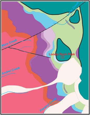
Figure 2. Geological map of the modeled area with geological cross-section traces.

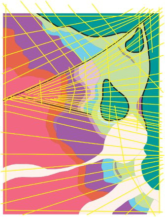
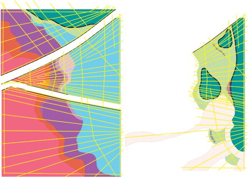
Figure 3. The area divided into four separate blocks for 3D modeling (also see Figure 4 – M3, M4, M5) and the corresponding geological cross sections.

A set of 54 geological cross sections were drawn (Figure 2) for reference in developing the 3D model.

GSI3D uses three methods for dealing with 3D models. Firstly, volumes in the model with top and base for a geological layer but without faults, it can calculate a non-volume model with only the base for a geological layer and separately, it can calculate the fault network.

In order to calculate a volume-based model, and still be able to use a fault network, we have generated the faults separately, outside of GSI3D.

To do that, the area was subdivided along the faults into three distinctive blocks. At the end, we have worked separately with a northern block, a central block and a southern block. The northern block is delimited along the north by the edge of the map, and south by a strike-slip fault. The central block is bounded by this strike-slip fault and a reverse fault to the south. The southern block, is delineated by this reverse fault and the southern edge of the map. (Figures 3 and 4 – M3, M4, M5)

Because the reverse fault affects only the Precambrian and Middle Jurassic formations, the central and southern blocks were delineated by the Wildflysch formation, Hășmaș nappe and Slides formation only as a reference. These units were modeled separately, afterwards. (Figures 3 and 4 – M4, M5)

Following this process, the resulting fault network and the four 3D geological models were imported into Move3D to make the final model edits and trim the faults depths.

4. Results

The purpose of using this methodology was to obtain a dynamic 3D geological model (Figures 4 and 5) that could be used to study the geology and allow further improvements (Main Map).

Figure 4. Final 3D geological model (The colors used are the same as the map). Notes: M1 – Compact 3D model showing the Hășmaș Granitoid, the Bukovinian nappe, the Hășmaș nappe, the Holocene slides and the faults. M2 – Compact 3D model showing the Bukovinian nappe, the Hășmaș nappe, the Holocene slides and the faults. M3 – Compact 3D model of northern block (see Figure 4) without the Hășmaș Granitoid. M4 – Compact 3D model of central block (see Figure 4) without the Hășmaș Granitoid. M5 – Compact 3D model of southern block (see Figure 4) without the Hășmaș Granitoid. M6 – Compact 3D model showing only the Bukovinian nappe and the faults. M7 – Compact 3D model showing only Hășmaș nappe, Holocene slides and the faults.

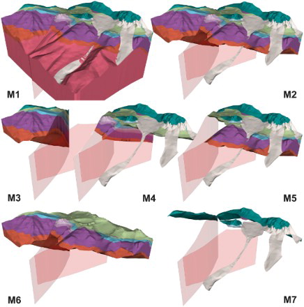
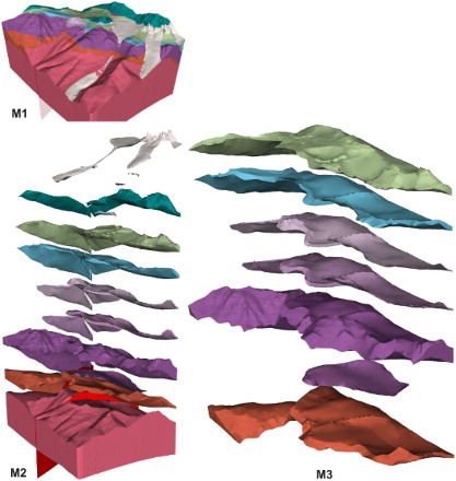
Figure 5. Final 3D geological model (The colors used are the same as the map). Notes: M1 – Compact 3D model showing the Hășmaș Granitoid, the Bukovinian nappe, the Hășmaș nappe, the Holocene slides and the faults. M2 – Exploded 3D model showing the Hășmaș Granitoid, the Bukovinian nappe, the Hășmaș nappe, the Holocene slides and the faults. M3 – Exploded 3D model showing only the Bukovinian nappe.

The model provides information regarding both the (1) spatial distribution of rock units, the relationship between them, and their relationship with faults and (2) calculate accurate volumes and unit bounding surfaces.

By modeling with GSI3D and Move3D, we obtained: (1) a primary stratigraphic sequence of the study area; (2) complete correlation of formation in geological cross sections; (3) cartographic boundaries of formations, both at the land surface and at depth.

After making this model we were able to calculate the volumes and surfaces for each unit (Table 1).

Table 1. Volumes and surfaces for the units utilized in the 3D model.

No.	Name	Area (km^2)	Volume (km^3)
1	Holocene – slides	0.48850	0.00815
2	Tithonian – lower cretacic – limestone	0.69293	0.06360
3	Kimmperidgian – limestone	0.03397	0.00062
4	Lower Induan – limestone (nappe)	0.01399	0.00057
5	Albian – barremian – the wildflysch formation	1.42911	0.17033
6	Basalt (from the wildflysch formation)	0.01116	0.00007
7	Middle Jurassic – sanstone limestone	1.61349	0.10405
8	Upper Triassic – limestone and dolomite	1.43166	0.06606
9	Ladinian – limestone	1.39380	0.07061
10	Induan – olenekian – dolomite	2.44787	0.41339
11	Lower Induan – conglomerate and sandstone	0.47646	0.01298
12	Upper Paleozoic – Hășmaș breccia	2.74517	0.20073
13	Precambrian – Hășmaș granitoid	3.83883	2.26445

The measurements obtained from the 3D geological model can be used to simplify the reserves calculation in the prospecting and exploration phase in an area of interest, thus reducing the associated costs of these endeavors.

5. Conclusions

The ultimate goal of this research was to try to introduce a new concept concerning the observation and study of the deposits and tectonic structures, in this case for the Tulgheș-Hășmaș-Ciuc syncline, by approaching them in a volumetric 3D space.

The resulting 3D geological model will allow geologists to make measurements from any region, because future edits to the model can be performed interactively.

In order to investigate theories about the evolution of geological structures or faults in the study area, the model can be imported into other specialized 3D modeling software, where values of resistance, density, porosity, etc. can be assigned to each map unit. After this process, using the same tool it is possible to apply specific compression or distension forces to the units. From adjusting these forces, it is possible to determine the processes by which folds or faults formed, and even under what conditions the overthrusts occurred.

Moreover, the model can be used with other digital (spatial) information such as 3D representations of outcrop, spatial distribution of vegetation, and 3D CAD, to form a complete modeling environment that could be used by National Park Administrations for promoting tourism or protecting natural or sensitive areas. The 3D geological model is provided as an Adobe Acrobat 3D pdf file so measurements of length and angles can be made through an interactive environment. These measurements are fairly accurate (Appendix).

The 3D geological model it is not meant to replace existing geological mapping methods, but to improve the geologist's capacity to make better interpretations, and offer the possibility to make measurements with a higher degree of accuracy. The complexity of faults and structures in the area have only been partially explored and understood. It is expected continuing studies with significant time scheduled for field campaigns will reveal more details, and improve the overall model.

Software

GSI3D – From British Geological Survey

QUANTUM GIS – From Open Source Geospatial Foundation

MOVE3D – From Midland Valley Exploration Limited

Acknowledgements

The authors thank product support and development teams at the British Geological Survey (GSI3D) and Midland Valley Exploration Limited (Move 2015) for their support and help in troubleshooting the software.

Disclosure statement

No potential conflict of interest was reported by the authors.

ORCID

Tony-Cristian Dumitriu http://orcid.org/0000-0001-6312-9221

Mihai Brânzilă http://orcid.org/0000-0002-0260-7709

Dorin-Sorin Baciu http://orcid.org/0000-0003-1971-8007

Appendix

Instructions for viewing and interacting with the 3D model in Adobe Acrobat.

These 3D PDF files require Adobe Acrobat Reader or Professional 7.0 or later for 3D capabilities. Please note that Apple's Preview, Foxit Reader or pdf viewers built into Mozilla Firefox or Google Chrome cannot render 3D data, therefore you must download the pdf to your computer and use Adobe Acrobat to view it. A three-button or scrolling mouse is also highly recommended.

• To view and interact with the model, enable it by clicking the left button on the mouse.

• To disable the content (in order to limit the amount of information being redraw when the model is opened) click the right mouse and select Disable content.

• For better visualization, go to Edit, Preferences, 3D & Multimedia and check Enable double-side rendering.

• When the content is enabled, the user can interact with it by applying the tools that appear on the toolbar above the model. Additional tools can be accessed from the drop-down menu under Rotate, if the toolbar is not already expanded. This toolbar can be expanded by clicking the right button on the model and choosing Tools and Expand 3D Tools.

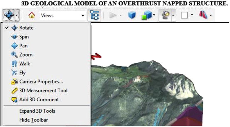
Notes: Rotate, Spin, Pan, Zoom, Fly (these five tools are used for moving the model or viewing it from different directions). 3D Measurement Tool which opens a new menu with tools from which the user can choose to measure length or angles.

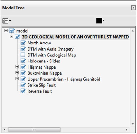
• When the content is enabled another menu appears left, named Model Tree (image below). This menu allows the user to enable or disable content from the 3D model by checking or unchecking the desired parts.

References

- Cohen, K. M., Finney, S. C., Gibbard, P. L., & Fan, J. X. (2014). The ISC international chronostratigraphic chart. Episodes, 36, 199–204. http://www.stratigraphy.org/icschart/chronostratchart2014–02.pdf
- Grasu, C., Miclăuș, C., Brânzilă, M., & Baciu, D. S. (2012). Tulgheș-Hășmaș-Ciuc Mesozoic Syncline: Geological monography. Edit. Univ. “Al. I. Cuza” Iași (in Romanian).
- Grasu, C., Turculeţ, I., Catana, C., & Niţă, M. (1995). The petrography of the mesozoic from “the external marginal syncline”. Edit. Acad. Rom., Bucureşti (in Romanian).
- Kessler, H., & Mathers, S. J. (2004). From geological maps to models – Finally capturing the geologists’ vision. Geoscientist, 14/10, 4–6. http://nora.nerc.ac.uk/983/
- Săndulescu, M. (1975). Geological survey of the central and northern part of the structure of Hăghimaș syncline (the Eastern Carpathians). An. Inst. Geol., XLV, Bucureşti. (in Romanian).
- Săndulescu, M., Mureșan, M., & Mureșan, G. (1975). Geological map of Romania, scale 1/50.000, Dămuc sheet. Inst. de Geol. şi Geofiz, Bucureşti (in Romanian).