White Glacier 2014, Axel Heiberg Island, Nunavut: mapped using Structure from Motion methods

ABSTRACT

We use Structure from Motion software to generate a new digital elevation model (DEM) of White Glacier, Axel Heiberg Island, Nunavut, using >400 oblique aerial photographs collected in July 2014. Spatially and radiometrically high-resolution imagery, optimized camera settings, low angle lighting conditions, and photo post-processing methods together supported the detection of small but distinct features on the surface of the snowpack and enabled feature matching during the image correlation process. The resulting DEM and orthoimage facilitated the production of a new 1:10,000 topographic map with 5 m vertical accuracy in the style of earlier cartographic works of White Glacier dating back to 1960. The new map of White Glacier will support calculation of the glacier's geodetic mass balance (mass change determined from ice volume change over the past 54 years) and provides an updated glacier hypsometry (area-elevation distribution) that will improve the accuracy of future mass balance calculations.

KEYWORDS:

• Structure from Motion
• photogrammetry
• mountain cartography
• Arctic
• glacier mapping
• snow-cover mapping

1. Introduction

White Glacier (79.45° N, 90.67° W) on Axel Heiberg Island, Nunavut, has been the subject of glaciological studies in Canada's north since 1959 and today hosts the longest mass balance record for an alpine glacier in the Canadian Arctic (55 years). It is one of 37 official reference glaciers within the Global Terrestrial Network for Glaciers through the United Nations Framework Convention on Climate Change. These observations, submitted annually to the World Glacier Monitoring Service (e.g. WGMS (2013) and previous issues), are used with others to calculate a worldwide glacier mass balance index, which is regularly published in climate change assessment reports (WGMS, 2008). Since the onset of the mass balance program, yearly measurements of snow accumulation and ice melt have been extrapolated across the White Glacier basin at its 1960 hypsometry and extent to calculate annual mass balance, save for an update to the hypsometry below 400 m above sea level (a.s.l.) in 2003 (Hember, Cogley, & Ecclestone, 2003). By producing a new map of the White Glacier basin and updating the hypsometry we can (1) improve the accuracy of future mass balance measurements and (2) reanalyze the historic record of observations using modeled estimates of hypsometry as it changed from 1960 to present (Zemp et al., 2013). A new map will also enable the calculation of geodetic mass balance, which is derived from ice volume change. This independent measure of mass change will allow us to assess quality of the historic mass balance record based on the consistency, or discrepancy, between the two methods.

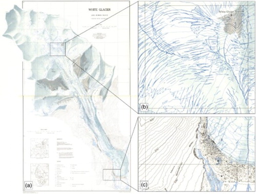
Airborne and ground-based surveying and mapping were important in the foundation and development of glaciological work at White Glacier. Early air photo surveys by the Royal Canadian Air Force in the summer of 1960 enabled the photogrammetric production of a series of six topographic maps of the Expedition Fiord Area on Axel Heiberg Island (Figure 1). The esthetic quality and cartographic caliber of the Expedition Fiord map series, including the 1:10,000 scale map of White Glacier by Haumann and Honegger (1964), pictured in Figure 2, are considered unprecedented in the Canadian Arctic for their era or indeed any time since (McKortel, 1963; Wheate, Alexander, Fisher, & Mouafo, 2001). Recently, digital versions of these six maps have been made available through the World Glacier Monitoring Service map database ‘Fluctuation of Glaciers Maps’ (http://www.wgms.ch/fog_maps.html), along with supporting texts describing the cartographic and photogrammetric methods of Haumann (1961), Haumann (1963), Blachut (1961), and Blachut (1963) used during these campaigns. Later surveys of ice elevations, conducted in 1969–1970 by Arnold (1981) to determine ablation rates and ice emergence velocities and in 2002–2003 by Hember et al. (2003) to determine the volume change of White Glacier below 400 m a.s.l., were restricted to the lower 4 km of the White Glacier terminus.

Figure 1. Location of White, Crusoe, Thompson, and Baby glaciers in the region of Expedition Fiord. Survey baseline points Astro 1 and Astro 2 are indicated, as is the location of the McGill Arctic Research Station. Background image: ASTER L1B composite, 5 July 2010.

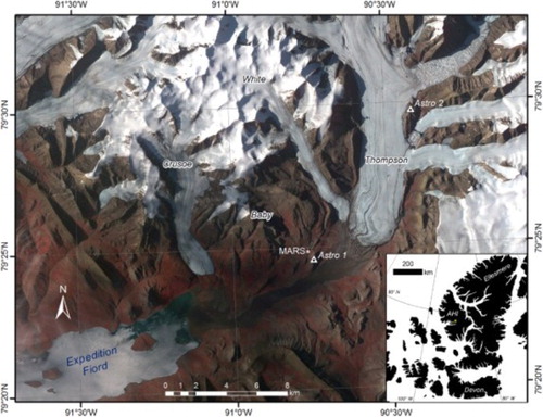
Figure 2. (a) Overview of White Glacier 1:10,000 (Haumann & Honegger, 1964), mapped in 1960 from ground surveys and photogrammetric techniques with examples of (b) detailed glacial features including supraglacial streams, crevasses, and the perennial snowline, and (c) the glacier terminus showing fault lines, proglacial streams and ponds, moraine and surface debris material, and survey cairns. Grid dimensions are 1 km x 1 km.

Now more than 50 years since the foundation of glaciological studies on Axel Heiberg Island, we present a new topographic map of White Glacier based on 2014 oblique aerial photography (Main Map). The topographic model for this map was produced using Agisoft's PhotoScan (version 1.1.0) Structure from Motion (SfM) software, which uses the principles of classical photogrammetry and takes advantage of computer automated image correlation analysis (Jebara, Azarbayejani, & Pentland, 1999). In recognition of the merit of the first 1:10,000 scale map of White Glacier by Haumann and Honegger (1964) we have strived to mimic the design features and quality of the original in our own map, while accepting the fundamental differences between hand-drawn and digital cartographic methods.

2. Methods

2.1. Air photo survey and image post-processing

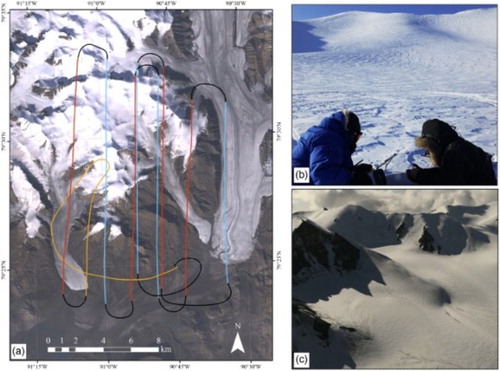
A Canon EOS 6D digital SLR camera equipped with an EF 24–105 mm f4 L IS USM lens (set to a focal length of 24 mm) was used to collect >500 oblique photographs of White Glacier from a Bell 206 L helicopter on 10 July 2014. At an average flying height of 1645 m a.s.l. (∼5400 ft), and a maximum altitude of 1990 m a.s.l. (∼6525 ft.) over the accumulation area, the camera achieved ground resolutions ranging from 0.05 to 0.52 m based on photos with a resolution of 3648 × 5472 pixels (20 Megapixels). An automatic intervalometer programmed to capture images every 3 seconds enabled 80% image overlap along-track and 60% across-track at an average flying speed of ∼150 km h⁻¹, as recommended in AgiSoft PhotoScan (hereafter, PhotoScan) User Manual and by Dr Matt Nolan (personal communication, 2014).

At the start of the survey, a reconnaissance flight was conducted over the Crusoe Glacier accumulation area (Figure 3(a)) to adjust the camera to settings that could detect features from the brightest part of the image (i.e. snow under direct sunshine). On the camera screen we were able to view the image exposure and RGB histograms on test photographs; through trial and error we found that camera settings of F-stop = F/10, ISO = 100 and a shutter speed of 1/2500 allowed for maximum contrast and detection of snow features across the accumulation area. These features included ripple marks (Figure 3(b)) and sastrugi, which were augmented by high-elevation surface melt and low angle lighting, as well as small slush avalanches and meltwater streams originating near nunataks. The low-exposure camera settings resulted in good definition in the accumulation area at the expense of under exposure in other locations, particularly in shadowed areas in the western tributary basins of White Glacier. However, the 14-bit radiometric resolution of the Canon EOS 6D enables over 16,000 tones to be uniquely identified, which supported the detection of subtle features in both snow-covered and shadowed regions. Using Canon Digital Photo Professional (version 3.12.51.2) photo editing software, the image brightness was increased by 30%, maintaining definition in the accumulation area while enhancing contrast in the shadowed regions of the glacier (Figure 3(c)). Batch post-processing was applied to ensure continuity in lighting throughout the photo series.

Figure 3. (a) Survey path on 10 July 2014, illustrating northbound flights in red, southbound flights in blue, and reconnaissance flight indicated in orange. (b) Example of sastrugi present in the accumulation of White Glacier with field team conducting snow pit analysis in foreground. (c) Provides an example survey photo demonstrating the detail and contrast possible from the accumulation area in both snow-covered and shadowed regions.

2.2. Model building

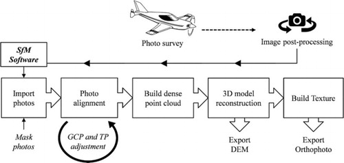
The SfM approach used by PhotoScan differs from traditional digital photogrammetry in that the image correlation analysis is used not only to derive three-dimensional (3D) structure from measureable feature offsets between images (i.e. parallax), but also to infer the camera position and calibration parameters of each photograph. This reduces the processing time required and enables projects to involve hundreds of photographs. Construction of a topographic model in PhotoScan is a multi-step process, as illustrated in Figure 4. Several iterations of model building for White Glacier were run before the final results were achieved; here, we describe the parameter settings and method used to produce the final product.

Figure 4. Workflow for the White Glacier model construction using Agisoft PhotoScan SfM Software.

With the reference projection defined as NAD27, the post-processed photographs were imported into PhotoScan and inspected for image coverage and quality, resulting in 473 photographs that were used to build the final model. Manually delineated image masks were applied to the photos to exclude features such as clouds and distant terrain outside the White Glacier basin that would interfere with photo alignment. In PhotoScan, photo alignment refers to the process in which a user-defined number of tie points, detected by correlation analysis between two photos, and camera orientation and positions are determined in 3D space using a bundle adjustment (PhotoScan User Manual). The resulting 3D point cloud calculated for a pair of images is referred to as a depth map, and PhotoScan amalgamates these depth maps to produce a sparse point cloud for the entire 3D structure to be modeled (PhotoScan User Manual). The most intensive and iterative phase of model building was adjusting and improving the photo alignment by the manual addition and removal of tie points (TPs) and ground control points (GCPs) (discussed in Section 2.4) and the deletion of erroneous points with high reprojection errors. In PhotoScan, reprojection error is a measure of localization accuracy in pixels. The standard assumption is that an ‘average reprojection error higher than 0.8 pix indicates quite inaccurate solution. Whereas reprojection error less than 0.5 is almost perfect’ (Agisoft Technical Support). The final sparse point cloud produced for White Glacier was reduced from over 3 million to approximately 2.5 million points, resulting in a final average reprojection error of 0.55 pixels.

With the derived camera positions resulting from the photo alignment (Figure 5(a)), a dense 3D point cloud was generated from depth maps created for each image pair, this time with the maximum number of tie points possible. The dense point cloud contained >200 million points over an area of approximately 100 km² (>2 points per m²). An internal tool within PhotoScan (‘Classify Ground Points’) was used to iteratively identify and filter out anomalous points that exceeded a 10 m radius and 45° inclination within a 100 m cell. These parameters were determined by trial and error and allowed for the preservation of topographic features while removing erroneous points resulting from image correlation mismatches.

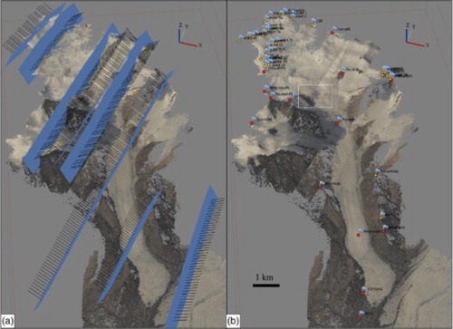
Figure 5. (a) Camera positions derived from the photo alignment bundle adjustment phase in Agisoft PhotoScan. Black lines indicate camera pointing direction and blue represents the camera faces. The Y-axis indicates geographic north. (b) Markers used to aid in photo alignment with red markers indicating GCPs and yellow markers indicating TPs. The white box indicates the location of the White Glacier icefall shown in Figure 6.

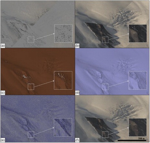
From the filtered dense point cloud, a 3D model was reconstructed using the Build Mesh function with the maximum number of model faces possible (>31 million) and interpolation of model voids enabled. Finally, a textured surface model, based on the Build Texture function, was produced using the average value of the pixels from individual photographs upon each model face. Figure 6 illustrates the intermediate and final products of PhotoScan model building near the White Glacier icefall, which features both ice and rock surfaces with varying degrees of complexity and slope.

Figure 6. Progression of intermediate products from PhotoScan including: (a) Sparse point cloud; (b) Dense point cloud; (c) Classified points (brown = ground points, white = unclassified); (d) Solid surface model; (e) Wireframe model; and (f) Textured model (Orthophoto).

2.3. Ground control and marker errors

GCPs, referred to as ‘Markers’ in PhotoScan, were selected from prominent features identifiable on both the 1960 White Glacier map and 2014 photographs. Fifteen GCPs and 38 tie points, amounting to 53 Markers, were used in the final photo alignment for the White Glacier basin following the iterative phase of Photo Alignment in PhotoScan (Figure 5(b)). The number of Marker projections (i.e. number of photographs where each Marker was manually identified) ranged from 4 to 95, with more than 50% of markers being detected in over 40 photographs.

Marker errors, defined as the discrepancy between defined and modeled GCP positions, ranged from 6.5 to 45.1 m (combined horizontal and vertical error), with an average error of 23.9 m. Marker errors increased for GCPs with high numbers of projections selected from photographs showing the target at distances exceeding 3–4 km, which resulted in the target feature being at a compromised resolution. However, we believed it to be important to incorporate as many projections as possible for each GCP to ensure continuity in the model.

2.4. Model results

We found that the SfM model construction generally performed well across the White Glacier basin, and surprisingly so across the accumulation area. The combination of low-exposure settings, high spatial and radiometric-resolution photography, low angle lighting, and the onset of summer surface melt generally resulted in successful feature matching and model construction throughout the snow-covered regions.

Erroneous sections of the model were found to be associated primarily with failures in survey design and photo coverage, rather than issues with the model building process. For example, two basins in the northeastern accumulation area of the glacier showed ‘pitted’ results, where the model returned regions of elevations significantly below (up to 100 m) the actual surface. In this case, image coverage of these basins was compromised by the eclipsing effect of ridges in the foreground of the oblique photographs. In another example, we found that along the western margin of the glacier trunk the model had difficulty transitioning smoothly from illuminated to shadowed lighting conditions, resulting in an artificial terrace in this region. Significant efforts were made to remedy this issue, including (1) adjusting the brightness and contrast parameters, (2) the inclusion of tie points, and (3) adjusting the selection parameters for ground points, but these proved to be ineffective. These two cases exemplify the most extreme and extensive model errors, yet together they comprise only 3% of the mapped basin area. Smaller isolated instances of ‘pitting’ on the scale of 50–400 m in length appear primarily in the accumulation area, and in some cases appear to be associated with variable cloud coverage between photographs. Our approach to managing these issues is addressed in Section 4.2, which describes contour construction and design.

The resulting 3D model and textured surface were exported as a digital elevation model (DEM) and orthophoto, respectively. The default model export cell size provided by Agisoft was 0.769 m, but we chose to export the DEM at a resolution of 5 m to reduce the impact of small-scale noise and variability on contour construction. The orthophoto was exported at a resolution of 1 m to facilitate the detailed mapping of small-scale features such as supraglacial streams and crevasses.

3. Map construction and design

The White Glacier 2014 1:10,000 map was produced entirely in Esri's ArcMap 10.1 from a combination of manually digitized features as well as data products generated by a variety of ArcMap tools. In this section we describe the steps taken to produce the map and the accuracy of the final product. We have endeavored to mirror the original 1960 map by Haumann (1961) in terms of both style and structure while updating the extent, hypsometry, and surface features of White Glacier.

3.1. Coordinate system and layout

The final data products (DEM and orthophoto) from PhotoScan were produced and exported to ArcMap with NAD27 geographic coordinates and reprojected into the local planar coordinate system used by Haumann and Honegger (1964). This system follows a Mercator projection with a central meridian of 269.2571944° E and latitude of origin of 79.4100306° N and respective false easting and northing values of 3000 and 60,000 m. The map is oriented to geographic north with a grid overlay divided into 1 km intervals. The extent of the final is 25,000 m E, 61,000 m N in the southwest, to 32,780 m E, 75,000 m N in the northeast (−90.987° E, 79.419° N; −90.605° E, 79.544° N). An interesting feature of the original map that we have maintained is the overflow of the northwestern-most basin of White Glacier 1.5 km beyond the western boundary of the neatline. We also chose to reproduce the two identical scale bars presented on the 1960 map, presumably because the original map was produced in two sheets that were divided latitudinally at 69,000 m N.

3.2. Contours

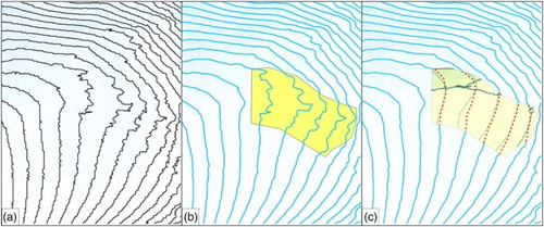
The Contour tool in ArcMap's Spatial Analysis toolbox was used to create 10 m contours from the imported PhotoScan DEM (raw contours shown in Figure 7(a)). These contours were then clipped to the contour extent of the 1960 map and smoothed using a Polynomial Approximation with Exponential Kernel (PAEK) filter with a 25 m threshold, which will interpolate along line paths of 25 m length (Figure 7(b)). Next, regions of model errors (i.e. voids) were identified and the erroneous contours produced in these regions were extracted using the Clip tool. We manually interpolated across these voids and in some cases used the contours of the 1960 map as a visual guide for the topographic structure of the area (Figure 7(c)). The final contours were colored according to land classification (rock = brown or ice = blue) with 100 m contours being represented with thicker line weights. Formlines, represented as dashed contour lines, indicate the areas where contours were interpolated across voids.

Figure 7. (a) Raw contours shown in black (10 m interval); (b) Smoothed contours with region of model errors highlighted in yellow; (c) Manually interpolated contours shown as red dashed lines overlain on an inset of the Haumann and Honegger (1964) map in the region of error. Contour interval = 10 m.

3.3. Relief shading

At the time of production, select maps in the 1960 Expedition Fiord map series were considered novel in North America for their inclusion of both relief shading and rock drawings (McKortel, 1963). Today, relief shading (also known as hill shading) is a common feature of topographic maps known to aid and accelerate map interpretation (Castner & Wheate, 1979). Using the Hillshade tool in ArcMap's Spatial Analysis toolbox, we produced separate relief shading products for rock and ice regions using an aspect of 280° and angle of 50°, which together achieved illumination and shading effects similar to those on the White Glacier 1960 map.

3.4. Glacial and proglacial features

Elements of the glacier surface and forefield were manually digitized in ArcMap as either polygon (p) or line (l) features. These include proglacial and supraglacial streams (l), crevasses (p), transverse and longitudinal ice structures (e.g. faults) (l), surface debris (p), and moraine materials (p). At this phase of map production, the fundamental differences between hand- and digitally produced cartography were obvious. Whereas the Haumann and Honegger (1964) map illustrated in great detail examples of rock-fall and debris cover, with individual rocks and boulders being depicted, we instead resorted to coarse and generic representations of surface debris and moraine material, accepting the futility of manually outlining such transitory small-scale features. Similar to the earlier map, we were unable to confidently represent the topography of particularly steep cliffs on the western margin of the glacier trunk and have therefore purposefully left these regions as blank voids labeled ‘Rock Wall’. However, the PhotoScan model did perform well in the eastern ‘Rock Wall’ region depicted in the 1960 map and we are therefore able to present the topography of that area for the first time. For historical context, we have also included a simple representation of the extent of the glacier terminus in 1960, as shown in the Haumann and Honegger (1964) map.

3.5. Survey cairns, spot elevations, and reference prisms

Ground surveys which provided ground control for the 1960 photogrammetry project made use of signal plates and a network of cairns, many of which were created in pairs to form survey baselines (e.g. I.C.B.N. and I.C.B.S., which we assume to signify Ice Cave Baseline North and South). We have chosen to include these reference points, as well as spot elevations, from the Haumann and Honegger (1964) map on our own, making it clear in the legend that these points are accurate as of their year of survey, 1960. It should be noted that the elevations of the 1960 spot elevations on the ice surface will have changed as a result of ice thinning or, in the case of Signal cairns W.G.F.4 and W.G.F.5, by the advance of Thompson Glacier into the White Glacier Forefield (W.G.F.) from the east. Several of the signal cairns that remain were resurveyed using a differential Global Positioning System (dGPS) system between 2011 and 2014. We include the point elevations of these contemporary surveys with a separate symbology. In all cases, our dGPS measurements of off-ice markers returned elevations within 1 m of those reported in Haumann and Honegger (1964), attesting to the high precision of the early work by the Swiss and Canadian surveyors on Axel Heiberg Island. We have added three new spot elevations at the sites of permanent reference prisms installed for our own total station surveys (R1–R3) and two spot elevations at historic markers we found that post-date the Haumann and Honegger (1964) map, including a meteorological station on the White Glacier Outwash Plain ‘W.G.O.P.’ used by Atsumu Ohmura in 1969 (Ohmura, 1981).

3.6. Map accuracy

As recommended by Agisoft, the standard rule of thumb for determining DEM accuracy from ground sampling distance (GSD) is 2x GSD in the horizontal and 4x in the vertical. Therefore, our GSD of 0.38 m (average ground resolution as calculated by PhotoScan) returns a horizontal accuracy of 0.76 m and vertical accuracy of 1.52 m. However, we believe this to be overly optimistic and more likely a reflection of DEM precision, not accuracy. The reported marker errors of the PhotoScan DEM product, which reflect the discrepancy between user defined and modeled GCPs, indicate average horizontal errors in longitude and latitude of 14.1 and 16.3 m, respectively, and an average elevation error of 10.5 m. These values, on the other hand, are subject to the unknown errors associated with the local plane coordinate system, which is poorly defined (Cogley & Jung-Rothenhausler, 2002), thereby introducing further errors in the geolocation of the model.

Ultimately, map accuracy can be considered as ‘the degree of conformity with a standard’ (Thompson, 1988). To determine how well our DEM conforms to our standard, the Haumann and Honegger (1964) map, we used the universal co-registration method developed by Nuth and Kääb (2011) and found that the standard deviation of elevation differences over stable terrain between our DEM and the 1960 map was 5.08 m following horizontal shifts on the order of 10–15 m. The necessity for these shifts are likely associated with the uncertainty in the estimated parameters of the local plane coordinate system and not inaccuracies in the DEM, considering the low reprojection error of 0.55 pixels that we were able to achieve in PhotoScan. With these considerations, we believe a reasonable generalization for the accuracy of the map to be 10 m vertically and 5 m horizontally.

4. Conclusions

Through the use of SfM photogrammetry methods applied to >400 oblique air photos, we have produced a DEM and orthoimage that together provide the foundation for a new 1:10,000 topographic map of White Glacier. Image correlation over the snow-covered areas of the glacier was possible due to the low-exposure camera settings, favorable lighting conditions, and melt season survey that enabled the detection of small-scale snow-surface features. Challenges faced in the process, which resulted in some localized model errors, were largely associated with flight survey design and uncertainties in the local plane coordinate system. Provided the opportunity to apply this technique in the future, nadir-oriented photography acquired from a greater flying height would resolve the issue of eclipsed regions, and map accuracy could be improved by the placement of more photo-identifiable GCPs. The co-registration technique developed by Nuth and Kääb (2011) provides an important tool in overcoming the coordinate system uncertainties of the Haumann and Honegger (1964) map as we move forward in calculating the volume change of White Glacier between 1960 and 2014 in future studies.

Software

The digital elevation model and orthoimage used to create the White Glacier 2014 1:10,000 map were produced using Agisoft PhotoScan version 1.1.0. Before importing into PhotoScan, the oblique photographs used in this study were post-processed in Canon Digital Photo Professional version 3.12.51.2. Map design and layout were accomplished in Esri ArcMap version 10.1.

Acknowledgements

Logistical support was provided by the Polar Continental Shelf Program (project of L. Copland), and we particularly thank Wayne Pollard for permission to work at the McGill Arctic Research Station and Miles Ecclestone for his assistance during the air photo survey. The authors are grateful for the comments of the reviewers and to G. Cogley and others whose previous works were instrumental in working with the Haumann and Honegger (1964) map.

Disclosure statement

No potential conflict of interest was reported by the authors.

Additional information

Funding

This research was supported by the Natural Sciences and Engineering Research Council of Canada (L. Copland, L. Thomson), Canada Foundation for Innovation (L. Copland), Ontario Research Fund (L. Copland), ArcticNet (L. Copland), the W. Garfield Weston Foundation (L. Thomson), and the Canadian Polar Commission's Northern Studies Training Program (L. Thomson).

References

- Arnold, K. C. (1981). Ice ablation measured by stakes and terrestrial photogrammetry – A comparison on the lower part of the White Glacier. Axel Heiberg Island, Canadian Arctic Archipelago. Axel Heiberg Island Research Reports, Glaciology, No.2, (Report No. 106).
- Blachut, T. J. (1961). Participation of the photogrammetric research section of the N.R.C. In B. S. Müller (Ed.), Preliminary report of 1959–60, Jacobsen-McGill Arctic research expedition to Axel Heiberg Island, Queen Elizabeth Islands (pp. 27–33). Montreal: McGill University.
- Blachut, T. J. (1963). Photogrammetric and cartographic results of the Axel Heiberg Island expedition. Canadian Surveyor, 17(2), 79–80.
- Castner, H. W., & Wheate, R. (1979). Re-assessing the role played by shaded relief on topographic scale maps. The Cartographic Journal, 16(2), 77–85. doi: 10.1179/caj.1979.16.2.77
- Cogley, J. G., & Jung-Rothenhausler, F. (2002). Digital elevation models of Axel Heiberg Island glaciers. Peterborough, Canada.
- Haumann, D. (1961). Co-ordinates of ground control points determined in 1960. In B. S. Muller (Ed.), Preliminary report of 1959–60, Jacobsen-McGill Arctic research expedition to Axel Heiberg Island, Queen Elizabeth Islands (pp. 35–42). Montreal: McGill University.
- Haumann, D. (1963). Surveying glaciers in Axel Heiberg Island. Canadian Surveyor, 17(2), 81–93.
- Haumann, D., & Honegger, D. (Cartographer). (1964). White Glacier, Axel Heiberg Island. Canadian Arctic Archipelago.
- Hember, R. A., Cogley, J. G., & Ecclestone, M. (2003). Volume balance of White Glacier terminus, Axel Heiberg Island, Nunavut, 1961–2003. Paper presented at the Eastern Snow Conference Proceedings.
- Jebara, T., Azarbayejani, A., & Pentland, A. (1999). 3D structure from 2D motion. IEEE Signal Processing Magazine, 16(3), 66–84. doi: 10.1109/79.768574
- McKortel, T. A. (1963). The reproduction of the Thompson Glacier map. Canadian Surveyor, 17(2), 93–95.
- Nuth, C., & Kääb, A. (2011). Co-registration and bias corrections of satellite elevation data sets for quantifying glacier thickness change. The Cryosphere, 5(1), 271–290. doi:10.5194/tc-5-271-2011
- Ohmura, A. (1981). Climate and energy balance on Arctic Tundra. Axel Heiberg Island Research Reports, 448.
- Thompson, M. M. (1988). Maps for America – Cartographic products of the U.S. Geological survey and others. (3rd ed). Washington, DC: U.S. Government Printing Office.
- WGMS. (2008). Global glacier changes: Facts and figures. Zurich: UNEP, World Glacier Monitoring Service.
- WGMS. (2013). Glacier mass balance bulletin no. 12 (2010–2011). Zurich, Switzerland.
- Wheate, R., Alexander, N., Fisher, M., & Mouafo, D. (2001). A brief history and progress of mountain cartography in Canada. Cartographica: The International Journal for Geographic Information and Geovisualization, 38(1–2), 31–39. doi:10.3138/N3L6-1874-5R18-118V
- Zemp, M., Thibert, E., Huss, M., Stumm, D., Rolstad Denby, C., Nuth, C., … Andreassen, L. M. (2013). Reanalysing glacier mass balance measurement series. The Cryosphere, 7, 1227–1245. doi: 10.5194/tc-7-1227-2013