Landscape diversity of the Czech Republic

ABSTRACT

This study presents an analysis and visual representation of landscape diversity in the Czech Republic. The Czech Republic is administratively subdivided into regions, which are further subdivided into districts; the basic territorial units used for the calculation of diversity were the districts. Landscape diversity was calculated from the freely available CORINE Land Cover (CLC) data for the Czech Republic. Additional data (the district and region layers) were taken from the digital vector geographic database of the Czech Republic ArcČR® 500. The Main Map (scale 1:600,000) shows landscape diversity calculated on the basis of Shannon entropy. For the purposes of visual representation, the effective number of categories in each district were calculated; the map also shows the prevailing type of land cover in each district. For comparison, an accompanying map shows landscape diversity at the regional level. Other accompanying maps contain information on CLC data, which is closely connected with landscape diversity. The four accompanying maps are at a scale of 1:1,800,000. Further information is also presented in addition to the maps (representation of CLC categories in the Czech Republic, brief texts characterizing the basic methodology used: CLC and the calculation of landscape diversity).

KEYWORDS:

• CORINE land cover
• landscape diversity
• Shannon index
• effective number of categories
• Czech Republic

1. Introduction

The landscape is a complex system of mutually interrelated and interdependent elements and components, which are both natural and anthropogenic in nature. Landscapes may be described and evaluated from various perspectives. Precise analyses of the structure and development of landscapes frequently use quantitative indicators enabling researchers to measure, quantify and evaluate certain characteristics of landscape structure. Quantitative characteristics of landscapes are determined by means of landscape metrics, which express the structure and development of a landscape. An advantage of quantitative indicators is that they enable researchers to obtain exact numerical data on landscape structure. The data can be compared for the same location in different years, or for different locations in the same year. Numerous landscape metrics are used – for example, McGarigal and Marks (1995) list 100 landscape metrics, though many of them are mutually interdependent (Cushman, McGarigal, & Neel, 2008).

One indicator of landscape quality is landscape diversity, which expresses the degree of heterogeneity and the structural variety of a landscape. Forman and Godron (1986) discuss the heterogeneity of individual landscapes – and their structural differentiation in terms of the distribution of species, energy and materials – in terms of the differences between landscape units. Landscape units may vary in size, shape, number, type and configuration. Determining this spatial distribution is an essential prerequisite for understanding the structure of a landscape – as well as for revealing the connections, relations, processes and flows occurring within the landscape as a whole.

The aim of this study is the spatial analysis of landscape diversity in the Czech Republic and especially the visualization of the results of this analysis. The study also includes the choice of methods for calculating and comparison of landscape diversity, the choice and design of methods for results visualization and clear representation of the data properties in accordance with Cauvin, Escobar, and Serradj (2010) and Dušek and Miřijovský (2009).

2. Calculation of landscape diversity

2.1. Methods of calculation

The basic concept for determining diversity originates in biology, where it is primarily applied to the determination of species diversity. Biologists use various methods to determine diversity, and it is not realistically possible to identify a single indicator that would be better than others (Duelli & Obrist, 2003). The most frequently used indicators are the following: the number of species; the Simpson index, which takes account of the more abundant species; and the Shannon index, which is sensitive to the occurrence of rare species (Farina, 2006). Diversity indices can also be applied to landscapes (UMass Landscape Ecology Lab, http://www.umass.edu/landeco).

The calculation and visual presentation of landscape diversity in the Czech Republic was based on the Shannon diversity index. This expresses information entropy (H) as defined by Claude E. Shannon (Shannon, 1948) and is applied to land cover data as follows:(1) $H=-1.\sum _{i=1}^n{p}_i.{\log }_{\mathrm{e}}{p}_i,$(1) where n is the number of land cover categories, p_i is the relative proportion of land cover category i ($0\le p_i\le 1,{\sum }_{i=1}^n{p}_i=1$), and log_e is the natural logarithm.

The Shannon index is associated with numerous theoretical problems (Dušek & Popelková, 2012). Nevertheless, it is one of the most frequently used methods of calculating diversity (Ricotta, 2005). The disadvantage of the Shannon index is the difficulty in interpreting the resulting values (Magurran, 2004). This is because the resulting values for the Shannon index are dependent on two parameters – the number of categories under investigation, and the evenness of representation of the individual categories across the given territory. The resulting values for different divisions of a particular territory may be identical. For this reason, when evaluating Shannon index values, it is essential to take account of the number of categories and the evenness of representation of the individual categories across the given territory.

In view of the difficulty of interpreting Shannon index values, the calculations of biodiversity are based on the effective number of species (Jost, 2006). This is the number of species (m) which, if evenly represented within a given territory, would attain the same value of diversity index.

Thus $p_1=p_2=\dots =p_m=1/m$, and then$H=-1.\sum _{i=1}^m{p}_i.{\log }_{\mathrm{e}}{p}_i=-1.m\left(\frac{1}{m}.{\log }_{\mathrm{e}}\frac{1}{m}\right)={\log }_{\mathrm{e}}m.$The effective number of species is calculated as follows:(2) $m=\exp \left(H\right)=\text{exp}\left(-1.\sum _{i=1}^n{p}_i.{\log }_{\mathrm{e}}{p}_i\right).$(2) The effective number of species is equivalent to the Hill number N₁ (Hill, 1973; Jost, 2006). When calculating landscape diversity, the number of species is replaced by the number of land cover categories. The effective number of categories is thus a theoretical, abstract number (i.e. not a whole number) of land cover categories at which evenly represented categories within a given territory would attain the same Shannon diversity index.

2.2. Territorial units’ choice

Despite attempts by some authors to give values of diversity for specific points, or for elementary surfaces in a grid (Rocchini et al., 2013), it is essential to calculate landscape diversity for selected areas; the diversity value depends on the size of these areas (Kallimanis & Koutsias, 2013). The selection of territorial units for the visual representation of diversity was based on three options: municipalities, districts and regions. A municipality (in Czech obec) is the basic (lowest-ranking) territorial unit of local government. The Czech Republic has 6258 municipalities with a mean area of 12.6 km². Given the scale of the CORINE Land Cover (CLC) data, the small size of municipalities means that they are not suitable for landscape diversity calculations. A region (in Czech kraj) is the largest (highest-ranking) territorial unit of local government in the Czech Republic; there are 14 regions, corresponding with NUTS3 units (Nomenclature of Units for Territorial Statistics). Unlike municipalities, regions are a suitable unit for diversity calculations; however, the considerable size differences between the regions (the ratio between the surface areas of the smallest and the largest region is 1:22) makes inter-regional comparison difficult. For this reason, landscape diversity on the regional level was shown in an accompanying map. A district (in Czech okres) is a lower-ranking territorial unit than a region; since 2003 districts have not had the status of local government territorial units, but they continue to be used as units for statistical (and certain other) purposes. There are 77 districts in the Czech Republic, with a mean area of 1024 km². The districts were chosen as the most suitable territorial unit for the depiction of landscape diversity, and they are shown in the Main Map.

2.3. Data

The map presents the results of an analysis of landscape diversity in the Czech Republic. Landscape diversity was calculated from freely available CLC data for the Czech Republic.

CLC is a European Union project coordinated by the European Environment Agency. CLC uses data from the LANDSAT satellite images to map land cover in Europe at a scale of 1:100,000. Additional information is taken from aerial photographs, maps and field research data. Land cover is described using a nomenclature consisting of 44 categories organized hierarchically in three levels; each category is assigned to one of five main CLC land cover classes. The five main classes – which comprise Level 1 (the highest level) in the hierarchy – are as follows: artificial surfaces, agricultural areas, forests and semi-natural areas, wetlands, and water bodies. Each of these main classes is then subdivided into categories which comprise Level 2 in the hierarchy, and these are in turn subdivided into categories which comprise Level 3 (each category in Level 3 is numbered with a three-digit numerical code). The most recent freely available land cover data are for 2012, when a total of 29 categories were recorded in the territory of the Czech Republic. The CLC 2012 layer used for this study (data from 2012), which is part of the Copernicus land monitoring service, was taken from the website of the Czech Environmental Information Agency (CENIA). CLC data are freely available to third parties on the basis of a Basic INSPIRE license (CENIA, 2016).

The district and region layers of the digital vector geographic database of the Czech Republic ArcČR® 500 were also used for the analysis of landscape diversity in the Czech Republic (the Czech Republic is administratively subdivided into regions, which are further subdivided into districts). The ArcČR® 500 database is at a scale of 1:500,000 and was created as a joint venture by three partners: the company ARCDATA PRAHA, s.r.o. (https://www.arcdata.cz/); the Land Survey Office; and the Czech Statistical Office. The database is freely available on the ARCDATA PRAHA website.

3. Creation of the cartographic work

3.1. Křovák’s projection

Křovák’s projection was used for both the Main Map and the accompanying maps. This is a conformal conic projection (Slocum, McMaster, Kessler, & Howard, 2005); however, it is not ideal for our application (an equal-area projection is preferable), but it is the official projection used in the Czech Republic for all civilian purposes, including the land register (cadastre) and state mapping. The maximum linear distortion is 14 cm per 1 km, and in view of the scale used, the difference between this projection and an equal-area projection is minimal.

3.2. Main map

The main aim of the study was to create a visual representation of landscape diversity in the territorial units of the Czech Republic. Because the interpretation of the resulting values of the Shannon diversity index is problematic, the Main Map shows the effective number of categories for each individual district. This is the number of land cover categories (m) at which evenly represented categories within a given territory would attain the same Shannon diversity index. The colour scale on the Main Map displays a comparison of the effective number of categories for the individual districts with the value for the entire Czech Republic (which is 6.19). The colour scale was designed according to Tyner (2010) and Brewer (1994). Geographical coordinates were added for better orientation on the map (Robinson, Morrison, Muehrcke, Kimerling, & Guptill, 1995).

In addition to the visual representation of diversity, the Main Map also shows the prevailing character of the landscape in each individual district. The prevailing CLC category indicates whether the territory is primarily agricultural, urban or forested. The effective number of categories is depicted using a colour scale, while the prevailing category is denoted by a point marker. In most maps, such markers tend to be placed at the centre of the area to which they pertain. However, this central positioning of the marker has the effect of breaking up the colour surface of the area, so a less common position was chosen instead. The point markers are located at the edge of the area to which they pertain (Figure 1). The basic shape of the marker consists of a segment from a circle, delineated by a circular arc and a base-line (a chord). Instead of a straight-line chord, the base-line of the marker is an irregular line whose precise course is determined by the edge of the area to which the marker pertains. The marker thus resembles a ‘peninsula’ or a ‘sunset’, protruding from the edge of the area towards the centre of the area. It clearly indicates the area to which it pertains, but it interferes minimally with the colour surface of the area itself (this colour conveys the main information contained in the map). One disadvantage of this method is the irregular base-line of the marker, which – if the marker were incorrectly positioned – could reduce the area covered by the marker and thus reduce the marker’s legibility (or have a detrimental effect on its aesthetic quality). In order to eliminate such problems as much as possible, the markers were added to the map in two steps:

1. The markers were not positioned at predetermined points in the area (e.g. at the southernmost point of the area). Instead, a suitable position was found in the southern, south-eastern or south-western sector of the area’s boundary line, along a relatively straight sector of the line.

2. The position of the central point of the circle in relation to the area boundary was selected in order to ensure that the coloured surface was the same for all the markers (i.e. 65% of the area of the circle, despite the irregular boundary lines). To determine the most suitable position of the central point of the circle, a script was written (using Matlab software) which moved the central point of the circle in small steps towards the boundary line until the required area (65%) was attained.

3.3. Accompanying maps and other elements of the cartographic work

The accompanying maps (scale 1:1,800,000) contain information that is closely connected with landscape diversity in the Czech districts. The maps are as follows:

• Landscape diversity in the regions of the Czech Republic – in order to enable comparison with the Main Map (showing values for the districts), the effective numbers of categories for each region (i.e. a higher-ranking territorial unit than a district) were depicted and compared with the value for the Czech Republic as a whole. The colour scale used in this map was the same as that used in the Main Map. The topographic base was created by Tolasz et al. (2007) and contains regional towns and rivers.

• Number of CLC categories and Number of CLC polygons – in order to ensure a consistent colour scheme for all the maps, the colours used in these maps are based on the colour of the predominant CLC category (Agricultural areas) used in the Main Map.

• Maximum and minimum diversity – the map shows the highest and lowest values of diversity, as well as identifying the individual districts by name. In order to prevent the map from becoming overfilled with names, the districts are numbered and a numbered list of the districts is given. The numbering of the districts is the numbering used by the Czech Statistical Office. A list of 77 district names in the map itself would have created a large area filled with text. For this reason the districts were listed around the frame of the cartographic work.

The Czech names feature a large number of diacritic marks above the letters (e.g. č, š, á, é, ů), and non-Czech (international) fonts do not always depict these diacritics with optimum clarity. For this reason an original Czech font was chosen for the list of district names and the other lettering in the maps. The font is Lido STF, designed by F. Štorm. This font is based on Times New Roman, but it has been redrawn with the Czech diacritics redesigned to ensure maximum legibility while maintaining the quality required of modern graphic design (Štorm, 2000).

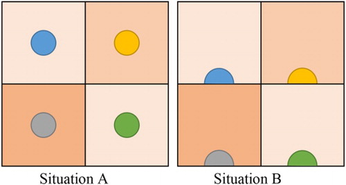
Figure 1. The difference between the perception of the coloured surface if the point marker is positioned in the centre of the area and at the boundary of the area. Situation A – the marker attracts attention and is dominant over the coloured surface. Situation B – the coloured surface is the dominant element.

The Main Map and accompanying maps also include further information. The representation of the CLC categories in the territory of the Czech Republic is shown in a table giving specific values. Each CLC category is listed along with the number of polygons in that particular category and the area covered by the category (in hectares and %). There is also brief text describing the methodology used: CLC and the method for calculating landscape diversity (effective number of categories).

The size of the cartographic work (A0 format) reflects the assumption that it will be read on two different levels (from a distance and in a close-up view). The more distant view will reveal the overall concept of the work, the main title will be legible, and the focus will be on the Main Map with the colour scale depicting landscape diversity; the map frame will appear as a grey line. On closer viewing, more detailed information will become visible on the Main Map and the accompanying maps; the content of the table will be legible, as will the text on CLC and landscape diversity as well as the list of districts in the map frame.

4. Conclusion

The most recent land cover data of the Czech Republic were processed for three levels of spatial resolution (state, region and district) and the results were presented in the Main Map. The resulting cartographic work – in the form of a wall map – presents data on landscape diversity in the Czech Republic in a clearly legible form. Landscape diversity calculated on the basis of Shannon entropy is depicted for the individual districts of the Czech Republic (in the Main Map) and the regions (in an accompanying map). The cartographic work also contains other information on CLC data closely connected with landscape diversity (accompanying maps, a table and texts).

In addition to standard cartographic methods, two relatively unusual methods were also used: the positioning of point markers (‘sunsets’) on the boundary of the areas to which they pertain, and the use of the map frame for the list of districts.

Software

The data were displayed, processed and analysed using Esri ArcGIS 10. Other software were used for the calculation of diversity: QGIS, Matlab and Microsoft Excel. Matlab was also used for calculating the position of the point markers on the area (district) boundaries (see Section 3.2).

Disclosure statement

No potential conflict of interest was reported by the authors.

Additional information

Funding

The map was created as part of the University of Ostrava project [SGS18/PřF/2015–2016].

References

- Brewer, C. A. (1994). Chapter 7 – color use guidelines for mapping and visualization. Modern Cartography Series, 2, 123–147. 10.1016/B978-0-08-042415-6.50014-4 doi: 10.1016/B978-0-08-042415-6.50014-4
- Cauvin, C., Escobar, F., & Serradj, A. (2010). New approaches in thematic cartography. London: ISTE and Hoboken.
- CENIA. (2016). Licence [online]. Retrieved from https://geoportal.gov.cz/web/guest/licence/
- Cushman, S. A., McGarigal, K., & Neel, M. (2008). Parsimony in landscape metrics: Strength, universality, and consistency. Ecological Indicators, 8, 691–703. doi: 10.1016/j.ecolind.2007.12.002
- Duelli, P., & Obrist, M. K. (2003). Biodiversity indicators: The choice of values and measures. Agriculture, Ecosystems and Environment, 98, 87–98. doi: 10.1016/S0167-8809(03)00072-0
- Dušek, R., & Miřijovský, J. (2009). Vizualizace prostorových dat: Chaos v dimenzích [ Visualization of geospatial data: Chaos in the dimensions]. Geografie-Sbornik, 114, 169–178. Retrieved from http://geography.cz/sbornik/clanky-z-geografie-20093-117/
- Dušek, R., & Popelková, R. (2012). Theoretical view of the Shannon index in the evaluation of landscape diversity. Acta Universitatis Carolinae, Geographica, 47(2), 5–13. Retrieved from http://www.aucgeographica.cz/index.php/AUC_Geographica/article/view/108
- Farina, A. (2006). Principles and methods in landscape ecology: Towards a science of the landscape. Dordrecht: Springer.
- Forman, R. T. T., & Godron, M. (1986). Landscape ecology. New York, NY: John Wiley.
- Hill, M. O. (1973). Diversity and evenness: A unifying notation and Its consequences. Ecology, 54, 427–432. doi: 10.2307/1934352
- Jost, L. (2006). Entropy and diversity. Oikos, 113, 363–375. doi: 10.1111/j.2006.0030-1299.14714.x
- Kallimanis A. S., & Koutsias, N. (2013). Geographical patterns of Corine land cover diversity across Europe: The effect of grain size and thematic resolution. Progress in Physical Geography, 37(2), 161–177. doi: 10.1177/0309133312465303
- Magurran, A. E. (2004). Measuring biological diversity. Oxford: Blackwell Publishing.
- McGarigal, K., & Marks, B. J. (1995). FRAGSTATS: Spatial pattern analysis program for quantifying landscape structure [PDF version]. Portland, OR: U.S. Department of Agriculture, Forest Service, Pacific Northwest Research Station. Retrieved from http://andrewsforest.oregonstate.edu/pubs/pdf/pub1538.pdf
- Ricotta, C. (2005). Through the jungle of biological diversity. Acta Biotheoretica, 53(1), 29–38. doi: 10.1007/s10441-005-7001-6
- Robinson, A. H., Morrison, J. L., Muehrcke, P. C., Kimerling, A. J., & Guptill, S. C. (1995). Elements of cartography. New York, NY: John Wiley & Sons.
- Rocchini, D., Delucchi, L., Bacaro, G., Cavallini, P., Feilhauer, H., Giles, M., … Neteler, M. (2013). Calculating landscape diversity with information-theory based indices: A GRASS GIS solution. Ecological Informatics, 17, 82–93. doi: 10.1016/j.ecoinf.2012.04.002
- Shannon, C. E. (1948). A mathematical theory of communication. The Bell System Technical Journal, 27, 379–423. doi: 10.1002/j.1538-7305.1948.tb01338.x
- Slocum, T. A., McMaster, R. B., Kessler, F. C., & Howard, H. H. (2005). 5. Upper Saddle River: Pearson Education.
- Štorm, F. (2000). Times s lidskou tváří II [Times with a human face II] [online]. Retrieved from http://lege.cz/typo/lido.htm
- Tolasz, R., Brázdil, R., Bulíř, O., Dobrovolný, P., Dubrovský, M., Hájková, L., … , Žalud, Z. (2007). Climate atlas of Czechia. Praha: Český hydrometeorologický ústav and Olomouc: Universita Palackého.
- Tyner, J. A. (2010). Principles of map design. New York, NY: The Guilford Press.