
ABSTRACT
This paper presents a glacial geomorphological map of landforms produced by the Lago General Carrera–Buenos Aires and Lago Cochrane–Pueyrredón ice lobes of the former Patagonian Ice Sheet. Over 35,000 landforms were digitized into a Geographical Information System from high-resolution (<15 m) satellite imagery, supported by field mapping. The map illustrates a rich suite of ice-marginal glacigenic, subglacial, glaciofluvial and glaciolacustrine landforms, many of which have not been mapped previously (e.g. hummocky terrain, till eskers, eskers). The map reveals two principal landform assemblages in the central Patagonian landscape: (i) an assemblage of nested latero-frontal moraine arcs, outwash plains or corridors, and inset hummocky terrain, till eskers and eskers, which formed when major ice lobes occupied positions on the Argentine steppe; and (ii) a lake-terminating system, dominated by the formation of glaciolacustrine landforms (deltas, shorelines) and localized ice-contact glaciofluvial features (e.g. outwash fans), which prevailed during deglaciation.
1. Introduction
The Patagonian Ice Sheet (PIS) has episodically expanded across the southern Andes of South America (38–56°S) throughout the Quaternary (; CitationCaldenius, 1932; CitationRabassa, 2008). During such times, substantial ice lobes advanced along major valleys constructing nested terminal moraine sequences and extensive outwash plains on the extra-Andean steppe (CitationCaldenius, 1932). Interest in these glacial landform assemblages has increased in recent years as information on the timing of glacier fluctuations may yield insight into past variations in Southern Westerly Wind changes (CitationBoex et al., 2013; CitationGarcía et al., 2012; CitationMoreno et al., 2009, Citation2015) and interhemispheric glacial and climate synchroneity (CitationDenton et al., 1999; CitationMurray et al., 2012; CitationSugden et al., 2005). Moreover, geomorphological studies, including glacial land-system approaches, have enabled detailed reconstructions of former ice dynamics (CitationBentley, Sugden, Hulton, & McCulloch, 2005; CitationDarvill, Stokes, Bentley, Evans, & Lovell, 2016; CitationLovell, Stokes, Bentley, & Benn, 2012). Whilst such methods have been applied in southernmost Patagonia, around central Patagonia and the North Patagonian Icefield (NPI) (∼46–48°S) previous work has focused on constraining the timing of glacial fluctuations, with less attention given to the detailed nature of landform-sediment assemblages (CitationGlasser, Harrison, & Jansson, 2009). Therefore, we aim to produce a comprehensive map of the glacial geomorphology related to two major ice lobes of central Patagonia. The map will provide the foundation for new reconstructions of ice lobe and palaeolake dynamics through the application of glacial inversion methods (CitationKleman et al., 2006) and land-system analysis (CitationEvans, 2003), and will underpin future chronological investigations.
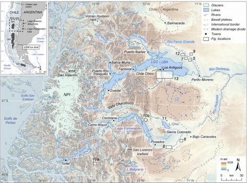
Figure 1. Location map of the studied area in central Patagonia. Boxes indicate the location and number of additional figures. Inset shows the extent of the Patagonian Ice Sheet (PIS) at the Last Glacial Maximum (LGM); redrawn after CitationSinger et al. (2004). The −125 m contour provides an indication of the approximate sea level drop at the LGM (e.g. CitationLambeck, Rouby, Purcell, Sun, & Sambridge, 2014; CitationPeltier & Fairbanks, 2006; CitationYokoyama, De Deckker, Lambeck, Johnston, & Fifield, 2001). NPI: North Patagonian Icefield; SPI: South Patagonian Icefield; CDI: Cordillera Darwin Icefield. Contemporary icefield limits extracted from the ‘Randolph Glacier Inventory’ dataset (CitationPfeffer et al., 2014).
2. Study location and previous work
2.1. Study location
The mapping conducted in this study focuses on the area between ∼46–48°S and ∼74–70°W (), a region characterized by both high mountains (>3–4000 m a.s.l) and deep troughs incised to below present sea level. The west of the study area is dominated by the modern NPI and its surrounding deep valleys and fjords (CitationGlasser & Ghiglione, 2009). These valleys feed into two major west-east trending overdeepened troughs occupied by the transnational lakes of Lago General Carrera–Buenos Aires (LGC-BA) and Lago Cochrane–Pueyrredón (LC-P). East of the Patagonian mountain front, the landscape transitions into a broad, semi-arid steppe interspersed with Plio-Pleistocene sedimentary and basalt plateaus (CitationGorring, Singer, Gowers, & Kay, 2003).
Previous studies indicate that fast-flowing outlet glaciers of an expanded PIS periodically occupied the LGC-BA and LC-P depressions (CitationGlasser & Jansson, 2005). These ice lobes advanced to the Argentine steppe (CitationCaldenius, 1932), blocked regional river systems and caused a ∼200 km westward shift in the drainage divide towards the Patagonian cordillera, which diverted meltwater eastward to the Atlantic Ocean (CitationBell, 2008; CitationGlasser et al., 2016; CitationTurner, Fogwill, McCulloch, & Sugden, 2005). During deglaciation, large proglacial lakes developed in the basins between terminal moraines and the ice front (CitationBell, 2008; CitationTurner et al., 2005). The eventual release of this freshwater to the Pacific Ocean disturbed vertical mixing patterns and regional climate (CitationGlasser et al., 2016).
2.2. Previous mapping
CitationCaldenius (1932) was the first to extensively map the glacial deposits of the region, providing the foundation for other early studies (CitationFeruglio, 1950; CitationFidalgo & Riggi, 1965). CitationCaldenius (1932) identified four terminal moraine systems on the Argentine steppe east of LGC-BA and LC-P, and argued that they formed over multiple glaciations based on their state of preservation. Since CitationCaldenius (1932), several studies have presented geomorphological maps from the region (), with mapping scale and detail tailored to specific research objectives ().
Figure 2. Extent and resolution of previous glacial geomorphological mapping studies, with mapped features listed in .
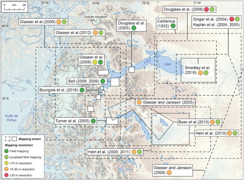
Table 1. Features mapped in previous studies.
Table 2. Summary of glacial geomorphology mapped in this study and criteria used in landform identification.
Table 3. Landforms mapped in this study classified according to depositional environment.
CitationGlasser and Jansson (2008) produced a map of glacial landforms formed at the margins and bed of the former PIS between 38 and 56°S, to infer ice-sheet scale ice dynamics (CitationGlasser, Jansson, Harrison, & Klemen, 2008). This map currently represents the most complete representation of glacial geomorphology at the ice lobe scale, but the low mapping resolution is such that subtle or complex features were necessarily omitted or generalized. For example, on the plains east of LGC-BA a complex system of ice-marginal meltwater channels and outwash corridors are noticeably simplified (CitationGlasser & Jansson, 2008).
Other studies have concentrated on smaller study areas around former glacier margins. For instance, CitationGlasser and Jansson (2005) mapped subglacial lineations across the LC-P ice lobe bed and inferred former ice-flow direction, regional ice-divide locations and ice thickness at local Last Glacial Maximum (LGM) extent. Similarly, and with the specific intention of supporting geochronological studies (; ), CitationKaplan, Ackert, Singer, Douglass, and Kurz (2004), CitationSinger, Ackert, and Guillou (2004) and CitationDouglass, Singer, Kaplan, Mickleson, and Caffee (2006) re-mapped the outer moraine complexes at LGC-BA. In addition, CitationHein et al. (2009, Citation2010), CitationHein, Dunai, Hulton, and Xu (2011) re-mapped the outer moraine systems of LC-P and identified a series of well-preserved moraine ridges, outwash terraces, palaeo-shorelines and landslide deposits. CitationHein et al. (2010) also noted some morphological differences between local LGM moraine sets, which included hummocky and sharp-crested forms.
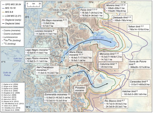
Figure 3. Major glacier limits and compilation of associated dating evidence based on previous studies. Cosmogenic nuclide exposure ages are presented as reported in original publications; however, where available, we report recalculated ages obtained from the use of southern hemisphere production rates (e.g. CitationKaplan et al., 2011; CitationPutnam et al., 2010). Luminescence ages are presented as reported in original publications. Published 14C determinations were recalibrated in Oxcal v4.3 (CitationBronk Ramsey, 2009) using the southern hemisphere calibration curve of CitationHogg et al. (2013). Arrows represent major ice lobe flow lines (CitationGlasser & Jansson, 2005).
Moraine ridges and other ice-contact landforms have also been mapped further west, in the Rio Bayo, Leones, Nef, Plomo and Colonia valleys, and at Lago Esmeralda ( and ), and dated to ascertain the timing of regional glacier readvances since the local LGM (CitationGlasser, Harrison, Schnabel, Fabel, & Jansson, 2012; CitationGlasser, Harrison, Ivy-Ochs, Duller, & Kubik, 2006). CitationTurner et al. (2005), CitationBell (2008) and, more recently, CitationGlasser et al. (2016), mapped palaeo-shorelines and raised lacustrine deltas formed at proglacial lake margins during glacier recession that contribute to a regional model of deglacial palaeolake development and drainage.
Several studies have mapped glacial landforms at the valley scale, close to contemporary icefields, to constrain the pattern of Holocene glacier fluctuations (e.g. CitationDavies & Glasser, 2012; CitationDouglass et al., 2005; CitationGlasser, Jansson, Harrison, & Rivera, 2005; CitationHarrison et al., 2006, Citation2008; CitationNimick, McGrath, Mahan, Friesen, & Leidich, 2016). Finally, CitationGlasser et al. (2009) compiled geomorphological and sedimentological evidence from 11 contemporary outlet glaciers to investigate the controls on landform formation around the NPI.
Overall, a lack of consistent, detailed mapping at the ice lobe scale has led to many important features (e.g. meltwater channels) being misidentified or overlooked in this region. Further mapping conducted at a high resolution (<15 m) is required for refined reconstructions of regional ice-sheet history and dynamics.
2.3. Ice lobe chronology
Across the study area, the timing of major ice lobe fluctuations is relatively well constrained owing to numerous dating studies (). Early palaeomagnetic studies at LGC-BA (CitationMörner & Sylwan, 1987, Citation1989) and LC-P (CitationSylwan, Beraza, & Casteli, 1991) established that some of the outer terminal moraines formed at the time of the Matuyama Reversed Chron over ∼780 ka ago (CitationSinger & Pringle, 1996). Subsequent 40Ar/39Ar dating of basaltic lava flows, interbedded within moraine sequences, provided additional constraints on the timing of ice lobe advances (CitationSinger et al., 2004; CitationTon-That, Singer, Mörner, & Rabassa, 1999). These studies dated the outermost moraines at LGC-BA to ∼1016 ka, and confirmed the timing of this ‘Greatest Patagonian Glaciation’, first recognized by CitationMercer (1976). At LGC-BA a further six terminal moraine sequences were deposited between ∼1016 and ∼760 ka, with another six formed between ∼760 and ∼109 ka (CitationSinger et al., 2004).
The chronology of major ice lobe fluctuations has since been refined through direct dating of glacial deposits, including cosmogenic nuclide exposure dating of moraine boulders (CitationBoex et al., 2013; CitationDouglass et al., 2006; CitationHein et al., 2010; CitationKaplan et al., 2004, Citation2011; CitationKaplan, Douglass, Singer, & Caffee, 2005) and outwash gravels (CitationHein et al., 2009, Citation2011), and luminescence dating of glaciofluvial outwash sediments (CitationGlasser et al., 2006; CitationHarrison, Glasser, Duller, & Jansson, 2012; CitationSmedley, Glasser, & Duller, 2016). These studies have supported the 40Ar/39Ar ages of earlier investigations, and provided evidence for additional ice lobe advances during MIS 2, 3, 6 and 8.
Recent studies have also attempted to constrain the pattern of glacier retreat following the local LGM (), and the consequent growth and drainage of ice-dammed proglacial lakes. The exact timing of glacier stillstands, and whether the retreat patterns of the LGC-BA and LC-P lobes were synchronous, however, remains equivocal. For example, CitationBoex et al. (2013) dated a stabilization of the LC-P lobe at the Maria Elena moraine (∼17.1 ka) in Valle Chacabuco. However, basal radiocarbon dates from lake basins that were exposed subaerially after ice retreat at this location have yielded older ages (∼19.8 cal ka; CitationVilla-Martínez, Moreno, & Valenzuela, 2012). Moreover, these radiocarbon dates are significantly older than either the exposure age of the Menucos moraine (∼16.9 ka; recalculated age cf. CitationKaplan et al., 2011), which represents an early deglaciation limit on the Argentine steppe at LGC-BA (), or the luminescence age of Menucos-related outwash deposits (∼14.2 ka; CitationSmedley et al., 2016). Similarly, CitationTurner et al. (2005) produced basal radiocarbon ages that exceed ∼12.8 cal ka from kettle holes at Lago Esmeralda and Cerro Ataud, and interpreted these dates as evidence for early deglaciation in this area. In contrast, CitationGlasser et al. (2012) proposed a regional stabilization of NPI outlet glaciers, including at this location, around the time of the European Younger Dryas, based on a suite of cosmogenic nuclide exposure ages of ∼11.0 to 12.8 ka, and supporting luminescence ages from local ice-contact deposits (CitationGlasser et al., 2006).
These alternative chronologies have hampered attempts to develop a coherent regional model of ice lobe and palaeolake evolution that reconcile all dating evidence (CitationBourgois, Cisternas, Braucher, Bourlès, & Frutos, 2016; CitationGlasser et al., 2016). New high-resolution mapping will enable refinements in the morphostratigraphic order of deglacial events and will contribute to resolving disparate retreat chronologies.
3. Methods
Geomorphological mapping was achieved through satellite image interpretation and field mapping. The map is presented at 1:420,000 scale using the WGS-1984 UTM-Zone18S coordinate system. Glacial landforms were digitized in ArcGIS (v10.3) at imaging scales of 1:8000 to 1:50,000, using a combination of 2.5 m resolution SPOT-5 and ∼1–2 m resolution DigitalGlobe (GeoEye-1, IKONOS) images available through the ESRI™ ‘World Imagery’ service. Areas of poor image quality (e.g. obscured by clouds) were examined in GoogleEarth™ software (v7.1), which also offers SPOT-5 and DigitalGlobe images for our study area. These image sources were used in preference to relatively low resolution satellite scenes (e.g. Landsat: 30 m) as they allowed a greater diversity of features to be mapped, and provided clarity in the identification of previously un-recorded, subtle landform types. Both relief-shaded (315° and 45° azimuth) and slope gradient-shaded models were constructed from ASTER G-DEMs (30 m cell-size) following procedures outlined in CitationSmith and Clark (2005), primarily to provide topographic context in areas of complex relief. Additionally, oblique three-dimensional views were created in GoogleEarth™ to aid landform identification, especially in areas where field verification was not possible.
4. Glacial geomorphology
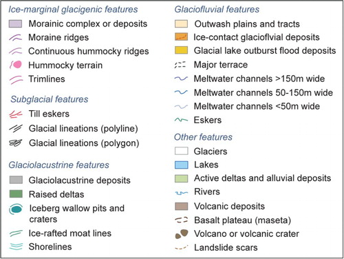
Fourteen main landform types were recorded on the geomorphological map (; ) and a total of 35,546 features (), which we describe herein. We also mapped trimlines, lakes, rivers, landslide scars and volcanic landforms including basalt mesetas, cones and lava flows, to provide further geological or topographic context.
Figure 4. Mapping legend to accompany . Note that on some figures, certain layers (e.g. ‘morainic complexes or deposits’) are not shown to enhance the visual clarity of our landform interpretations. Contemporary glacier extents were extracted from the ‘Randolph Glacier Inventory’ dataset presented in CitationPfeffer et al. (2014).
4.1. Moraine ridges
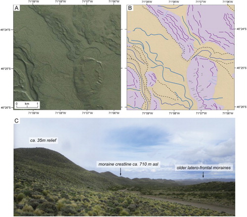
Prominent linear ridges of positive relief are interpreted as moraines that demarcate the limits of former glacier margins. Moraines can be single, cross-valley ridges, or occur within complex, multi-ridge systems. Moraines exhibit ∼5–40 m relief and sharp, level or undulating crests. Most often, moraines are closely spaced, with arcuate, crenulate or saw-tooth planforms (). The ice-contact face of prominent moraines can be adorned with low-relief hummocks, and in places are interspersed amongst larger assemblages of hummocky terrain (section 4.3). Elsewhere, moraine fragments exhibit weak barchanoid form, suggestive of overriding by active ice (CitationEvans, 2009). On the Argentine forelands around the main depressions, moraine complexes run continuously for tens of kilometres ((C)) and form tightly nested latero-frontal arcs (CitationKaplan, Hein, Hubbard, & Lax, 2009). These arcs are locally dissected by meltwater channels, which feed into ice-marginal outwash corridors or graded outwash plains (). The regional distribution of moraines reflects a pattern of westwards glacier retreat towards the modern NPI (CitationGlasser et al., 2012).
Figure 5. (A) Satellite image (DigitalGlobe 2015; ESRI™) and (B) mapped moraine ridges and outwash deposits from the northern margin of the LGC-BA lobe. Outwash occurs within narrow meltwater channels incised through moraines (left of image) or as broader lateral corridors between moraine sequences (centre left of image). Moraines are locally dissected by former meltwater streams (right of image) which feed into broad sandur plains. (C) View across latero-frontal moraine arc east of Puerto Ibañez with higher elevation (older) moraine sequence in distance (right of image).
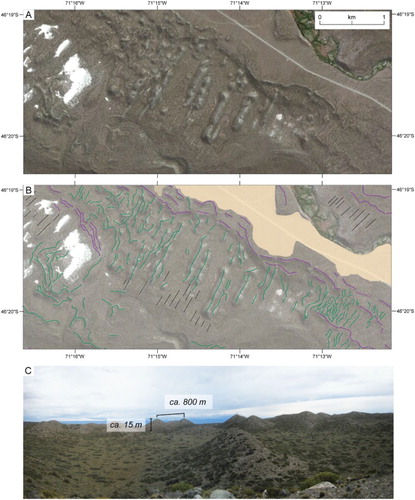
4.2. Continuous hummocky ridges
These features comprise accumulations of closely spaced hummocks and short (<300 m) ridges of moderate relief (∼5–25 m). Individual mounds can be difficult to delimit, but when viewed in planform represent semi-continuous parallel chains oriented perpendicular to ice flow (). Occasionally, high-relief, sharp-crested ridges are interspersed amongst continuous hummocky ridges These landforms may represent active push ridges fed by supraglacially dumped debris (e.g. CitationBoulton & Eyles, 1979; CitationLukas, 2005), perhaps in the absence of a widespread deforming layer.
Figure 6. (A) Satellite image (DigitalGlobe 2015; ESRI™) and (B) continuous hummocky ridges mapped along the southern LC-P ice lobe margin. The image shows numerous short ridges and hummocks that connect to generate longer ice-margin parallel chains when viewed in planform. Sequences of closely spaced ridges are separated by narrow lateral outwash corridors, whilst individual ridges may be separated by minor marginal meltwater channels of <50 m wide. The outer ridges (bottom right of image) are heavily dissected by meltwater channels which feed a lateral sandur plain. (C) View across continuous hummocky ridge chain, showing variable hummock height and lengths, and proglacial outwash deposits.
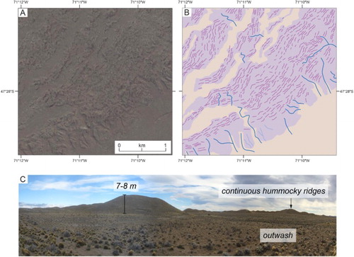
Alternatively, they could represent degraded moraines, or moraines that have been dissected by meltwater channels. Continuous hummocky ridges are exclusive to the southern LC-P margin, where they have previously been depicted as discrete, unbroken moraine ridges (CitationGlasser & Jansson, 2008; CitationHein et al., 2010).
4.3. Hummocky terrain
Several forms of hummocky terrain were identified around former ice margins. Small-scale hummocks () are more common, and consist of densely spaced circular to semi-rounded hills of <10 m relief. The hummocks are largely chaotic, but may be organized into crude arcuate bands. Push moraines are often dispersed amongst the more chaotic hummocks. Large-scale hummocky terrain () is limited to a small zone on the southern LC-P margin, and consists of densely spaced irregular hummocks (polygons) and ridges (polylines) with intervening depressions. Hummocks range from 5–30 m high and 10–200 m wide and form chaotic assemblages. Their morphology is varied, and includes circular or oval-shaped mounds and linear ridges with straight or corrugated crests. These deposits are morphologically comparable to hummocky terrain produced by stagnant glacier snouts that foundered into saturated basal tills (CitationEyles, Boyce, Barendregt, 1999; CitationBoone and Eyles, 2001).
Figure 7. (A) Satellite image (DigitalGlobe 2013; ESRI™) and (B) mapped hummocky terrain on the northern LGC-BA ice lobe margin. These small-scale hummocks are largely chaotic but may be organized into crude arcuate bands (top left of image) that are interspersed with low-relief push moraine ridges.
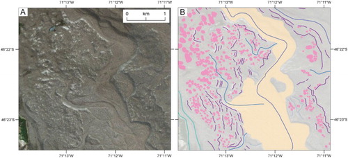
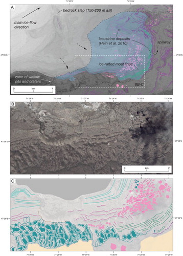
Figure 8. (A) Context for landform interpretation along the southern LC-P ice lobe margin, east of Posados. Late LGM glacier and proglacial lake limit after CitationHein et al. (2010), based on the identification of lacustrine deposits (black circles). At the time of the reconstruction, CitationHein et al. (2010) suggest ice was grounded around a prominent north–south trending bedrock step, and experienced insufficient flux to fully occupy the upper basin. The lake level contour (625 m a.s.l) was extracted from an ASTER-GDEM model. The extent of (B) and (C) is indicated by the dashed white box. (B) Satellite image (DigitalGlobe 2013; ESRI™) and (C) mapped landforms, showing a complex arrangement of geomorphic features. The right-hand section of the image shows an assemblage of densely spaced circular or oval-shaped mounds and linear ridges that display morphological resemblance with examples of ice-stagnation hummocky terrain (CitationEyles et al., 1999; CitationBoone and Eyles, 2001). The hummock assemblage merges into a large complex of inferred iceberg wallow pits and craters, which exhibit deep semi-circular to elongate depressions and are enclosed by high-relief rim ridges or lateral berm ridges (e.g. CitationBarrie et al., 1986; CitationWoodward-Lynas et al., 1991). Low-relief hummock chains are interpreted as moat line ridges deposited at the margins of a small ice-contact lake ice (cf. CitationHall, Hendy, & Denton, 2006). Inferred moat line ridges occur outside the limits of hummocky terrain, and along the ice-contact face of prominent sharp-crested ridges. Their distribution and ‘shoreline-like’ pattern (A) is consistent with the perimeter and estimated water level of the proglacial lake system mapped by CitationHein et al. (2010).
4.4. Till eskers
These features are straight-to-sinuous ridges with undulating crests, of between 50–500 m long and 5–15 m high. The ridges are orientated oblique to outer moraine crests, but not parallel with former ice-flow indicators (). The ridges often merge into, or closely align with the limbs of saw-tooth moraines. These features are present on adverse topographic slopes inside larger, sharp-crested moraine ridges along the northern LGC-BA margin. Based on their morphology, we interpret these landforms as infilled water conduit systems, or so-called ‘till eskers’, as identified in modern Icelandic settings (CitationChristoffersen, Piotrowski, & Larsen, 2005; CitationLarsen, Piotrowski, Christoffersen, & Menzies, 2006; CitationEvans, Ewertowski, & Orton, 2016). Their origin is hypothesized to reflect the squeezing of saturated till into elongated basal cavities or R-channels after meltwater abandonment (CitationEvans, Nelson, & Webb, 2010). Data on the sedimentary nature of these landforms could test our current interpretation.
Figure 9. (A) Satellite image (DigitalGlobe 2012; ESRI™) and (B) mapped landforms on the northern margin of the LGC-BA lobe. Image shows saw-tooth push moraines and straight-to-sinuous inset ridges that align sub-parallel to former ice-flow direction, and are interpreted as preserved till eskers as recorded on some modern glacier forelands (CitationChristoffersen et al., 2005; CitationEvans et al., 2016).
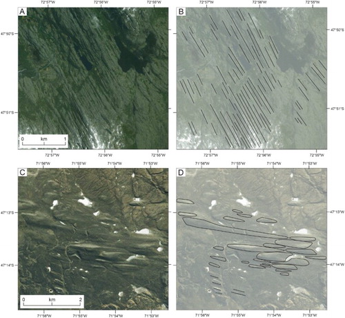
4.5. Glacial lineations
Linear, parallel, positive relief landforms displaying high-directional conformity were mapped as glacial lineations (). Their regional distribution mirrors the principal ice-discharge pathways along major W-E trending valley axes (CitationGlasser & Jansson, 2005). Bedrock lineations are well developed in areas of ice-scoured terrain and range from ∼200–3000 m long and ∼30–100 m wide. Tightly clustered oval-shaped drumlins and flutes are identified near the Chacabuco-Pueyrredón junction, and around the base of Sierra Colorado. Subdued sediment flutings (1–3 m high) occur on the Argentine forelands between moraine ridges (), though they are difficult to detect, even within high-resolution imagery.
Figure 10. Examples of glacial lineations from across the study area. (A) Satellite image (DigitalGlobe 2014; ESRI™) and (B) mapped lineations formed in bedrock south of Los Ñadis. (C) Satellite image (DigitalGlobe 2015; ESRI™) and (D) mapped lineations formed in sediment at the junction of Valle Chacabuco and the Pueyrredón basin.
4.6. Meltwater channels
Straight, sinuous or meandering channels that are devoid on contemporary drainage and begin and end abruptly are interpreted as meltwater channels. In total, we map 1736 channels, which are ubiquitous around former ice lobe margins. Channel length reaches ∼30 km and channel width ranges from ∼20 to 800 m, the widest forming corridors of outwash-infill and converging with broader outwash plains (). Meltwater channels follow former ice margins () or issue from frontal moraine systems. Along the southern LGC-BA margin, meltwater incision has eroded all but certain localized upstanding moraine fragments. Here, ice-marginal meltwater channels provide a clearer indication of former glacier position and surface gradient than moraines (Main Map; e.g. CitationBentley et al., 2005; CitationDarvill, Stokes, Bentley, & Lovell, 2014).
4.7. Outwash plains and tracts
Broad, gently sloping surfaces of glaciofluvial sand and gravel represent outwash plains and tracts. Around the NPI, outwash deposits mantle the floor of major erosional corridors (CitationGlasser et al., 2009). On former glacier forelands, coalescent outwash fans prograde eastwards from latero-frontal moraine complexes to form extensive outwash plains (; CitationCaldenius, 1932; CitationHein et al., 2009, Citation2011; CitationSmedley et al., 2016), or occur within ice-margin parallel corridors due to topographic constraints (e.g. moraines; ). Outwash deposits may be pitted, either in narrow ice-marginal strips, or at fan apices, due to melt-out of buried glacier ice (CitationEvans & Orton, 2015; CitationEvans & Twigg, 2002). The surfaces of outwash plains are often imprinted with complex abandoned channel networks, or exhibit clear terrace levels (). These features may record the evolution of the proglacial drainage system, reflecting changes in glacier margin position, ice-marginal topography, or meltwater discharge (CitationEvans & Twigg, 2002).
4.8. Eskers
These features are described as straight-to-sinuous ridges with oblique orientation relative to former ice-flow direction. Ridges can be isolated landforms () or occur within dense networks (). These features are inset behind outer moraine crests along the northern LGC-BA and LC-P margins. Whilst no open sections were identified in the field, the ridge surfaces contained sands, gravels and cobbles. We interpret these landforms as eskers (e.g. CitationStorrar, Evans, Stokes, Ewertowski, 2015), but acknowledge that only a single esker has been identified previously in Patagonia (CitationClapperton, 1989; CitationDarvill et al., 2014; CitationLovell, Stokes, & Bentley, 2011).
Figure 11. (A) Satellite image (DigitalGlobe 2017; Bing Maps™) from the northern margin of the LC-P lobe and (B) mapped landforms. The image shows a prominent, positive relief, sinuous ridge interpreted as an esker, alongside multiple smaller esker ridges. Ice-flow direction was from left to right.
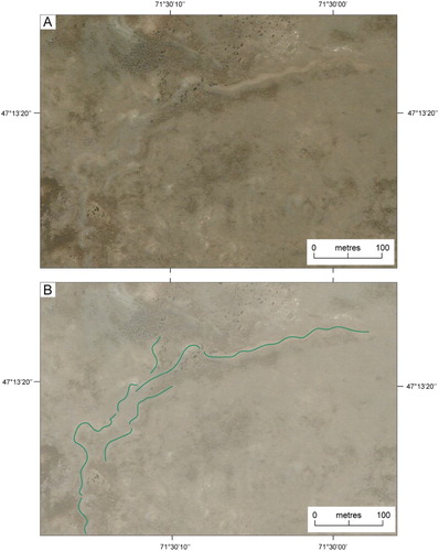
Figure 12. (A) Satellite image (DigitalGlobe 2013; ESRI™) from the northern margin of the LGC-BA lobe and (B) interpretation of the glacial geomorphology. The image shows push moraine ridges, inset eskers and sediment flutings. The inferred eskers range from sinuous ridges that are either isolated or occur within complex networks (lower right of image), to more enigmatic, near-straight ridges and conical mounds (centre of image) of comparatively high relief (C).
An additional zone of enigmatic landforms was mapped at LGC-BA. These features form a densely spaced complex of near-straight ridges and conical mounds, ranging from 20 to 150 m wide and 100 to 800 m long (). The ridges are characterized by hummocky long-profiles and variable widths, and their surfaces comprise sand and gravel sediments. These features might represent large-scale crevasse fills (cf. CitationBennett, Huddart, Waller, 2000); however, we speculate that they are eskers.
Their existence alongside another inferred esker network, shown in (B), might support this interpretation.
4.9. Ice-contact outwash deposits
Gently sloping terraces of glaciofluvial sand and gravel, perched on valley sides or at valley confluences, are interpreted as ice-contact outwash deposits. These accumulations represent ice-contact glaciofluvial depo-centres and include: pitted, valley-side kame terraces; outwash fans with pitted ice-contact slopes (outwash heads; sensu CitationKirkbride, 2000); and low-gradient subaqueous fans draped over low-lying bedrock outcrops. These landforms occur within narrow valleys around the modern NPI, their location perhaps a reflection of favourable topographic setting (e.g. valley narrowings; cf. CitationBarr & Lovell, 2014). Examples occur at Lago Brown, Lago Esmeralda and at the Colonia-Baker confluence (Main Map). Such deposits are often considered to have formed during periods of temporary glacier stabilization (CitationSpedding & Evans, 2002).
4.10. Glacial lake outburst flood deposits
Large-scale gravel bars or flat-topped accumulations that exhibit channelized surfaces and imbricated boulder lags, with boulders of 1–10 m height, are interpreted as Glacial lake outburst flood deposits (e.g. CitationHarrison et al., 2006). Such accumulations are elevated above the modern Río Baker west of Valle Chacabuco, and northwest of Cochrane (Main Map).
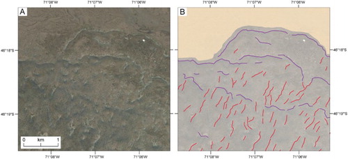
4.11. Iceberg wallow pits and craters
These landforms consist of semi-circular pits or elongated craters of between 5 and 35 m depth, flanked by semi-circular ring-ridges, or steep-sided (>35°) lateral berm ridges (). The structures occur within a densely spaced network of regular NNW-SSE orientation, approximately sub-parallel to former ice-flow direction (CitationHein et al., 2010). These features occur along a narrow sector of the southern LC-P margin, where based on the distribution of lacustrine sediments, CitationHein et al. (2010) have mapped the extent of a small ice-marginal lake at ∼625 m a.s.l ((A)). We interpret the landforms as iceberg grounding structures. In glaciomarine settings, these include various pits, craters and scours (CitationWoodward-Lynas, Josenhans, Barrie, Lewis, & Parrot, 1991). When embedded in the seafloor, icebergs excavate deep depressions due to vertical (impact) loading and wave-induced horizontal loading that facilitates iceberg rotation and wallowing, and sediment displacement to form berm ridges (e.g. CitationBarrie, Collins, Clark, Lewis, & Parrot, 1986; CitationClark & Landva, 1988). Our morphologically based interpretation is consistent with the presence of a transient lake system at this site (CitationHein et al., 2010).
4.12. Ice-rafted moat lines
Around the margins of the small ice-contact lake mapped by CitationHein et al. (2010), we have identified curvilinear chains of closely spaced, low-relief (<4 m) small ridges and mounds, which are discontinuous but can be linked together and run for ∼100–700 m (). In contrast to other linear features (e.g. moraines), these curvilinear chains are more subdued, less continuous and are not sharp-crested. Given the ice-marginal lacustrine context and their morphological nature, we interpret these landforms as moat lines of ice-rafted debris let down through the unfrozen margins of an ice-contact lake (cf. CitationHall, Hendy, Denton, 2006). Sedimentological analyses are needed to test this interpretation.
4.13. Shorelines
Continuous linear terraces that run unbroken for tens of kilometres and exhibit no positive relief are interpreted as wave-cut scarps and benches (CitationGlasser & Jansson, 2008). The most prominent lake shorelines occur east of LGC-BA and LC-P () and rise to ∼300 m higher than contemporary lake levels. Previous shoreline mapping has enabled several reconstructions of proglacial lake evolution (CitationBourgois et al., 2016; CitationGlasser et al., 2016; CitationTurner et al., 2005). In comparison, we mapped a greater number of shoreline features, including very faint, closely spaced shoreline fragments located between the major wave-cut scarps. These features are only discernible from high-resolution images and hint at a complex lake level history.
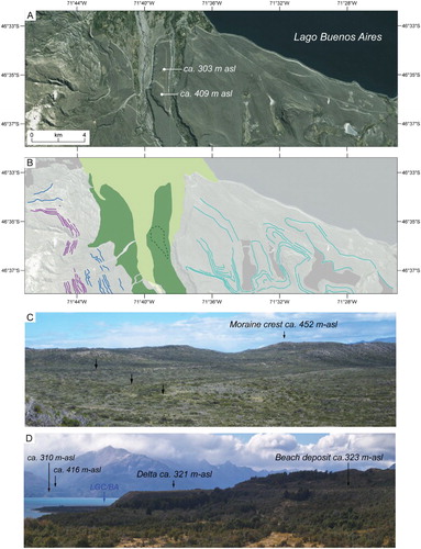
Figure 13. (A) Satellite image (DigitalGlobe 2014; ESRI™) and (B) mapped glaciolacustrine landforms along the southern margin of Lago General Carrera–Buenos Aires. Features include raised deltas, wave-cut lake shorelines and areas of lacustrine sediment accumulation within palaeolake embayments. Also note the high-level lateral moraine ridges and marginal meltwater channels of the southern LGC-BA lobe margin. Field photos of (C) former lake shorelines cut into glacigenic deposits and (D) raised lacustrine deltas and adjacent beach deposits formed in the mouths of tributary valleys of Lago General Carrera–Buenos Aires. The ca. 310 and 321 m deltas are coeval though have experienced different amounts of postglacial uplift. The ca. 416 m delta pre-dates the lower elevation features and records stepped lake level lowering.
4.14. Raised deltas
Flat-topped, sediment accumulations in the mouths of tributary valleys, and perched above modern lakes, represent raised lacustrine deltas (; CitationBell, 2008, Citation2009; CitationGlasser et al., 2016; CitationHein et al., 2010; CitationTurner et al., 2005). At LGC-BA, raised deltas are often flanked by beaches ((D)). Narrow, wave-cut terraces are present on some delta fronts, and are cited as evidence of either staged lake lowering (CitationBell, 2008) or lake transgression (CitationBourgois et al., 2016).
4.15. Glaciolacustrine deposits
On satellite imagery, glaciolacustrine deposits are flat, pale-coloured sediment accumulations deposited in former proglacial lakes (; Main Map). Field sections confirm the presence of glaciolacustrine sediments. Significant glaciolacustrine accumulations occur around former ice margins, palaeolake embayments (), and on valley sides, where they drape bedrock or glacigenic deposits.
5. Summary and conclusions
This paper presents a new glacial geomorphological map (Main Map) of the central Patagonian region. Mapping is conducted at a consistent, high level of detail that exceeds that of previous works, and encompasses the complete area occupied by two major outlet lobes of the former PIS. The map reveals a complex suite of landform assemblages that includes (i) previously unmapped components of the glacial geomorphological record (e.g. continuous hummocky ridges, hummocky terrain, till eskers, eskers and iceberg features); and (ii) updated spatial and morphological representations of features mapped previously from lower resolution imagery (e.g. moraines, meltwater channels). This new evidence allows the preliminary sub-division of mapped landform assemblages into two principal assemblages. (1) An outer assemblage developed on the former ice lobe forelands documents the evolution of piedmont glaciers emerging from mountainous catchments. This assemblage contains nested latero-frontal moraine arcs and associated glaciofluvial outwash tracts, with localized eskers and till eskers inset behind larger moraine complexes. (2) An inner assemblage that developed as ice margins retreated into overdeepened valleys in the western sector of the study area, and led to evolution of a glaciolacustrine environment. This assemblage comprises widespread raised deltas, shorelines and fine-grained glaciolacustrine sediment piles. In addition, ice-contact glaciofluvial depo-centres (e.g. subaqueous fans) were constructed in topographically favourable locations (e.g. valley narrowings). Beyond these preliminary findings, the new geomorphological dataset presented here will facilitate the application of glacial inversion methods (CitationKleman et al., 2006) and, for the first time, land-system analysis (CitationEvans, 2003) at the ice lobe scale. We anticipate that the dataset will be used to produce detailed reconstructions of (i) ice-margin recession; (ii) evolving ice-dynamics; and (iii) evolving palaeolake systems.
Software
Landforms were recorded in Esri ArcGIS (v10.3) and final map production undertaken in Adobe Illustrator.
Shapefiles.zip
Download Zip (8.7 MB)The glacial geomorphology of the Lago Buenos Aires and Lago Pueyrredón ice lobes of central Patagonia.pdf
Download PDF (116.4 MB)Acknowledgements
JMB would like to thank Aaron Bendle for field assistance, in addition to Dave Evans (Durham University, UK) and Gerardo Benito (Consejo Superior de Investigaciones Científicas, Spain) for insightful discussion about the origin of some landforms. We thank Christopher Darvill, Krister Jansson and Nick Scarle for careful reviews that improved the overall quality of the paper and map. We also thank Chris Clark for clear editorial guidance throughout the review process.
Disclosure statement
No potential conflict of interest was reported by the authors.
ORCID
Jacob M. Bendle http://orcid.org/0000-0002-3572-7192
Additional information
Funding
Related Research Data
References
- Barr, I. D., & Lovell, H. (2014). A review of topographic controls on moraine distribution. Geomorphology, 226, 44–64. doi: 10.1016/j.geomorph.2014.07.030
- Barrie, J. V., Collins, W. T., Clark, J. I., Lewis, C. F. M., & Parrot, D. R. (1986). Submersible observations and origin of an iceberg pit on the grand banks of Newfoundland. Current Research, Part A, Geological Survey of Canada, Paper 86-1A, 251–258.
- Bell, C. M. (2008). Punctuated drainage of an ice-dammed quaternary lake in Southern South America. Geografiska Annaler Series A Physical Geography, 90(1), 1–17. doi: 10.1111/j.1468-0459.2008.00330.x
- Bell, C. M. (2009). Quaternary lacustrine braid deltas on lake general Carrera in Southern Chile. Andean Geology, 36(1), 51–65.
- Bennett, M. R., Huddart, D., & Waller, R. I. (2000). Glaciofluvial crevasse and conduit fills as indicators of supraglacial dewatering during a surge, Skeiðarárjoökull, Iceland. Journal of Glaciology, 46, 25–34. doi: 10.3189/172756500781833232
- Bentley, M. J., Sugden, D. E., Hulton, N. R. J., & McCulloch, R. D. (2005). The landforms and pattern of deglaciation in the Strait of Magellan and Bahía Inútil, Southernmost South America. Geografiska Annaler: Series A, Physical Geography, 87, 313–333. doi: 10.1111/j.0435-3676.2005.00261.x
- Boex, J., Fogwill, C., Harrison, S., Glasser, N. F., Hein, A., Schnabel, C., & Xu, S. (2013). Rapid thinning of the late Pleistocene Patagonian Ice Sheet followed migration of the Southern Westerlies. Scientific Reports, 3. doi:10.1038/srep02118.
- Boone, S. J., & Eyles, N. (2001). Geotechnical model for great plains hummocky moraine formed by till deformation below stagnant ice. Geomorphology, 38, 109–124. doi: 10.1016/S0169-555X(00)00072-6
- Boulton, G. S., & Eyles, N. (1979). Sedimentation by valley glaciers: A model and genetic classification. In C. Schuchter (Eds.), Moraines and varves (pp. 11–23). Balkema: Rotterdam.
- Bourgois, J., Cisternas, M. E., Braucher, R., Bourlès, D., & Frutos, J. (2016). Geomorphic records along the general Carrera (Chile)–Buenos Aires (Argentina) glacial lake (46°–48° S), climate inferences, and glacial rebound for the past 7–9 ka. The Journal of Geology, 124, 27–53. doi: 10.1086/684252
- Bronk Ramsey, C. (2009). Bayesian analysis of radiocarbon dates. Radiocarbon, 51, 337–360. doi: 10.1017/S0033822200033865
- Caldenius, C. C. (1932). Las glaciaciones cuaternarios en la Patagonia y Tierra del Fuego. Geografiska Annaler, 14, 1–164. doi: 10.2307/519583
- Christoffersen, P., Piotrowski, J. A., & Larsen, N. K. (2005). Basal processes beneath an Arctic glacier and their geomorphic imprint after a surge, Elisebreen, Svalbard. Quaternary Research, 64, 125–137. doi: 10.1016/j.yqres.2005.05.009
- Clapperton, C. M. (1989). Asymmetrical drumlins in Patagonia, Chile. Sedimentary Geology, 62, 387–398. doi: 10.1016/0037-0738(89)90127-9
- Clark, J. I., & Landva, J. (1988). Geotechnical aspects of seabed pits in the grand banks area. Canadian Geotechnical Journal, 25, 448–454. doi: 10.1139/t88-050
- Darvill, C. M., Stokes, C. M., Bentley, M. J., Evans, D. J. A., & Lovell, H. (2016). Dynamics of former ice lobes of the southernmost Patagonian Ice Sheet based on a glacial landsystems approach. Journal of Quaternary Science. doi: 10.1002/jqs.2890
- Darvill, C. M., Stokes, C. R., Bentley, M. J., & Lovell, H. (2014). A glacial geomorphological map of the southernmost ice lobes of Patagonia: The Bahía Inútil–San Sebastián, Magellan, Otway, Skyring and Río Gallegos lobes. Journal of Maps, 10, 500–520. doi: 10.1080/17445647.2014.890134
- Davies, B. J., & Glasser, N. F. (2012). Accelerating shrinkage of Patagonian glaciers from the little ice age (∼AD 1870) to 2011. Journal of Glaciology, 58, 1063–1084. doi: 10.3189/2012JoG12J026
- Denton, G. H., Heusser, C. J., Lowell, T. V., Moreno, P. I., Andersen, B. G., Heusser, L. E., Schluchter, C., & Marchant, D. R. (1999). Interhemispheric linkage of paleoclimate during the last glaciation. Geografiska Annaler Series A Physical Geography, 81, 107–153. doi: 10.1111/j.0435-3676.1999.00055.x
- Douglass, D. C., Singer, B. S., Kaplan, M. R., Ackert, R. P., Mickelson, D. M., & Caffee, M. W. (2005). Evidence of early Holocene glacial advances in Southern South America from cosmogenic surface-exposure dating. Geology, 33, 237–240. doi: 10.1130/G21144.1
- Douglass, D. C., Singer, B. S., Kaplan, M. R., Mickleson, D. M., & Caffee, M. W. (2006). Cosmogenic nuclide surface exposure dating of boulders on last-glacial and late-glacial moraines, Lago Buenos Aires, Argentina: Interpretative strategies and paleoclimate implications. Quaternary Geochronology, 1, 43–58. doi: 10.1016/j.quageo.2006.06.001
- Evans, D. J. A. (2003). Glacial landsystems. London: Hodder-Arnold.
- Evans, D. J. A. (2009). Controlled moraines: Origins, characteristics and palaeoglaciological implications. Quaternary Science Reviews, 28, 183–208. doi: 10.1016/j.quascirev.2008.10.024
- Evans, D. J., Ewertowski, M., & Orton, C. (2016). Fláajökull (north lobe), Iceland: active temperate piedmont lobe glacial landsystem. Journal of Maps, 12, 777–789.
- Evans, D. J. A., Nelson, C. D., & Webb, C. (2010). An assessment of fluting and ‘till esker’ formation on the foreland of Sandfellsjökull, Iceland. Geomorphology, 114, 453–465. doi: 10.1016/j.geomorph.2009.08.016
- Evans, D. J. A., & Orton, C. (2015). Heinabergsjökull and Skalafellsjökull, Iceland: Active temperate piedmont lobe and outwash head glacial landsystem. Journal of Maps, 11, 415–431. doi: 10.1080/17445647.2014.919617
- Evans, D. J. A., & Twigg, D. R. (2002). The active temperate glacial landsystem: A model based on Breiðamerkurjökull and Fjallsjökull, Iceland. Quaternary Science Reviews, 21, 2143–2177. doi: 10.1016/S0277-3791(02)00019-7
- Eyles, N., Boyce, J. I., & Barendregt, R. W. (1999). Hummocky moraine: sedimentary record of stagnant Laurentide Ice Sheet lobes resting on soft beds. Sedimentary Geology, 123, 163–174. doi: 10.1016/S0037-0738(98)00129-8
- Feruglio, E. (1950). Descripción geológica de la Patagonia. Dirección General de Yacimientos Petroliferos Fiscales (Tomo, III, pp. 1–342). Buenos Aires: Editora Coni.
- Fidalgo, F., & Riggi, J. (1965). Los rodados patagónicos de la Maesta de Guenguel y airededores (Santa Cruz). Revista de la Asociación Geológica Argentina, 20, 273–325.
- García, J. L., Kaplan, M. R., Hall, B. L., Schaefer, J. M., Vega, R. M., Schwartz, R., & Finkel, R. (2012). Glacier expansion in Southern Patagonia throughout the Antarctic cold reversal. Geology, 40, 859–862. doi: 10.1130/G33164.1
- Glasser, N. F., & Ghiglione, M. C. (2009). Structural, tectonic and glaciological controls on the evolution of fjord landscapes. Geomorphology, 105, 291–302. doi: 10.1016/j.geomorph.2008.10.007
- Glasser, N. F., Harrison, S., Ivy-Ochs, S., Duller, G. A., & Kubik, P. W. (2006). Evidence from the Rio Bayo valley on the extent of the North Patagonian Icefield during the late Pleistocene-Holocene transition. Quaternary Research, 65, 70–77. doi: 10.1016/j.yqres.2005.09.002
- Glasser, N. F., Harrison, S., & Jansson, K. N. (2009). Topographic controls on glacier sediment–landform associations around the temperate North Patagonian Icefield. Quaternary Science Reviews, 28, 2817–2832. doi: 10.1016/j.quascirev.2009.07.011
- Glasser, N. F., Harrison, S., Schnabel, C., Fabel, D., & Jansson, K. N. (2012). Younger Dryas and early Holocene age glacier advances in Patagonia. Quaternary Science Reviews, 58, 7–17. doi: 10.1016/j.quascirev.2012.10.011
- Glasser, N. F., & Jansson, K. (2005). Fast-flowing outlet glaciers of the last glacial maximum Patagonian Icefield. Quaternary Research, 63, 206–211. doi: 10.1016/j.yqres.2004.11.002
- Glasser, N. F., & Jansson, K. (2008). The glacial map of southern South America. Journal of Maps, 4, 175–196. doi: 10.4113/jom.2008.1020
- Glasser, N. F., Jansson, K. N., Duller, G. A. T., Singarayer, J., Holloway, M., & Harrison, S. (2016). Glacial lake drainage in Patagonia (13-8 kyr) and response of the adjacent Pacific Ocean. Scientific Reports, 6, 289. doi: 10.1038/srep21064
- Glasser, N. F., Jansson, K. N., Harrison, S., & Klemen, J. (2008). The glacial geomorphology and Pleistocene history of Southern South America between 38°S and 56°S. Quaternary Science Reviews, 27, 365–390. doi: 10.1016/j.quascirev.2007.11.011
- Glasser, N. F., Jansson, K. N., Harrison, S., & Rivera, A. (2005). Geomorphological evidence for variations of the North Patagonian Icefield during the Holocene. Geomorphology, 71, 263–277. doi: 10.1016/j.geomorph.2005.02.003
- Gorring, M., Singer, B., Gowers, J., & Kay, S. M. (2003). Plio-Pleistocene basalts from the Meseta del Lago Buenos Aires, Argentina: Evidence for asthenosphe-lithosphere interactions during slab window magmatism. Chemical Geology, 193, 215–235. doi: 10.1016/S0009-2541(02)00249-8
- Hall, B. L., Hendy, C. H., & Denton, G. H. (2006). Lake-ice conveyor deposits: Geomorphology, sedimentology, and importance in reconstructing the glacial history of the Dry Valleys. Geomorphology, 75, 143–156. doi: 10.1016/j.geomorph.2004.11.025
- Harrison, S., Glasser, N. F., Duller, G. A., & Jansson, K. N. (2012). Early and mid-Holocene age for the Tempanos moraines, Laguna San Rafael, Patagonian Chile. Quaternary Science Reviews, 31, 82–92. doi: 10.1016/j.quascirev.2011.10.015
- Harrison, S., Glasser, N. F., Winchester, V., Haresign, E., Warren, C. R., Duller, G. A. T., … Kubik, P. (2008). Glaciar León, Chilean Patagonia: Late Holocene chronology and geomorphology. The Holocene, 18, 643–652. doi: 10.1177/0959683607086771
- Harrison, S., Glasser, N. F., Winchester, V., Haresign, E., Warren, C. R., & Jansson, K. N. (2006). A glacial lake outburst food associated with recent mountain glacier retreat, Patagonian Andes. The Holocene, 16, 611–620. doi: 10.1191/0959683606hl957rr
- Hein, A. S., Dunai, T. J., Hulton, N. R. J., & Xu, S. (2011). Exposure dating outwash gravels to determine the age of the greatest Patagonian glaciations. Geology, 39, 103–106. doi: 10.1130/G31215.1
- Hein, A. S., Hulton, N. R. J., Dunai, T. J., Schnabel, C., Kaplan, M. R., Naylor, M., & Xu, S. (2009). Middle Pleistocene glaciation in Patagonia dated by cosmogenic-nuclide measurements on outwash gravel. Earth and Planetary Science Letters, 286, 184–197. doi: 10.1016/j.epsl.2009.06.026
- Hein, A. S., Hulton, N. R. J., Dunai, T. J., Sugden, D. E., Kaplan, M. R., & Xu, S. (2010). The chronology of the last glacial maximum and deglacial events in central Argentine Patagonia. Quaternary Science Reviews, 29, 1212–1227. doi: 10.1016/j.quascirev.2010.01.020
- Hogg, A. G., Hua, Q., Blackwell, P. G., Niu, M., Buck, C. E., Guilderson, T. P., … Turney, C. S. (2013). SHCal13 Southern hemisphere calibration, 0–50,000 years cal BP. Radiocarbon, 55, 1–15.
- Kaplan, M. R., Ackert, R. P., Singer, B. S., Douglass, D. C., & Kurz, M. D. (2004). Cosmogenic nuclide chronology of millennial-scale glacial advances during O-isotope stage 2 in Patagonia. Bulletin of the Geological Society of America, 116, 308–321. doi: 10.1130/B25178.1
- Kaplan, M. R., Douglass, D. C., Singer, B. S., & Caffee, M. W. (2005). Cosmogenic nuclide chronology of pre-last glacial maximum moraines at Lago Buenos Aires, 46°S, Argentina. Quaternary Research, 63, 301–315. doi: 10.1016/j.yqres.2004.12.003
- Kaplan, M. R., Hein, A. S., Hubbard, A., & Lax, S. M. (2009). Can glacial erosion limit the extent of glaciation? Geomorphology, 103, 172–179. doi: 10.1016/j.geomorph.2008.04.020
- Kaplan, M. R., Strelin, J. A., Schaefer, J. M., Denton, G. H., Finkel, R. C., Schwartz, R., & Travis, S. G. (2011). In-situ cosmogenic 10 Be production rate at Lago Argentino, Patagonia: Implications for late-glacial climate chronology. Earth and Planetary Science Letters, 309, 21–32. doi: 10.1016/j.epsl.2011.06.018
- Kirkbride, M. P. (2000). Ice marginal geomorphology and Holocene expansion of debris-covered Tasman Glacier, New Zealand. In M. Nakawo, C. Raymond, & A. Fountain (Eds.), Debris-covered glaciers (pp. 211–217). Wallingford: IAHS Publication 264.
- Kleman, J., Hättestrand, C., Stroeven, A. P., Jansson, K. N., De Angelis, H., & Borgström, I. (2006). Reconstruction of palaeo-ice sheets – inversion of their glacial geomorphological record. In P. Knight (Ed.), Glacier Science and Environmental Change (pp. 192–198). Oxford: Blackwell.
- Lambeck, K., Rouby, H., Purcell, A., Sun, Y., & Sambridge, M. (2014). Sea level and global ice volumes from the last glacial maximum to the Holocene. Proceedings of the National Academy of Sciences, 111, 15296–15303. doi: 10.1073/pnas.1411762111
- Larsen, N. K., Piotrowski, J. A., Christoffersen, P., & Menzies, J. (2006). Formation and deformation of basal till during a glacier surge; Elisebreen, Svalbard. Geomorphology, 81, 217–234. doi: 10.1016/j.geomorph.2006.04.018
- Lovell, H., Stokes, C. R., & Bentley, M. J. (2011). A glacial geomorphological map of the Seno Skyring-Seno Otway-Strait of Magellan region, Southernmost Patagonia. Journal of Maps, 7, 318–339. doi: 10.4113/jom.2011.1156
- Lovell, H., Stokes, C. R., Bentley, M. J., & Benn, D. I. (2012). Evidence for rapid ice flow and proglacial lake evolution around the central Strait of Magellan region, Southernmost Patagonia. Journal of Quaternary Science, 27, 625–638. doi: 10.1002/jqs.2555
- Lukas, S. (2005). A test of the englacial thrusting hypothesis of ‘hummocky’ moraine formation: Case studies from the Northwest Highlands, Scotland. Boreas, 34, 287–307. doi: 10.1080/03009480510013042
- Mercer, J. H. (1976). Glacial history of Southernmost South-America. Quaternary Research, 6, 125–166. doi: 10.1016/0033-5894(76)90047-8
- Moreno, P. I., Denton, G. H., Moreno, H., Lowell, T. V., Putnam, A. E., & Kaplan, M. R. (2015). Radiocarbon chronology of the last glacial maximum and its termination in Northwestern Patagonia. Quaternary Science Reviews, 122, 233–249. doi: 10.1016/j.quascirev.2015.05.027
- Moreno, P. I., Kaplan, M. R., Francois, J. P., Villa-Martinez, R., Moy, C. M., Stern, C. R., & Kubik, P. W. (2009). Renewed glacial activity during the Antarctic cold reversal and persistence of cold conditions until 11.5 ka in Southwestern Patagonia. Geology, 37, 375–378. doi: 10.1130/G25399A.1
- Mörner, N., & Sylwan, C. (1987). Revised terminal moraine chronology at Lago Buenos Aires, Patagonia, Argentina. International Project on Paleolimnology and Late Cenozoic Climate, 4, 15–16.
- Mörner, N., & Sylwan, C. (1989). Magnetostratigraphy of the Patagonian moraine sequences at Lago Buenos Aires. Journal of South American Earth Sciences, 2, 385–389. doi: 10.1016/0895-9811(89)90016-3
- Murray, D. S., Carlson, A. E., Singer, B. S., Anslow, F. S., He, F., Caffee, M., … Otto- Bliesner, B. L. (2012). Northern hemisphere forcing of the last deglaciation in Southern Patagonia. Geology, 40, 631–634. doi: 10.1130/G32836.1
- Nimick, D. A., McGrath, D., Mahan, S. A., Friesen, B. A., & Leidich, J. (2016). Latest Pleistocene and Holocene glacial events in the Colonia valley, Northern Patagonia Icefield, Southern Chile. Journal of Quaternary Science, 31, 551–564. doi: 10.1002/jqs.2847
- Peltier, W. R., & Fairbanks, R. G. (2006). Global glacial ice volume and last glacial maximum duration from an extended Barbados sea level record. Quaternary Science Reviews, 25, 3322–3337. doi: 10.1016/j.quascirev.2006.04.010
- Pfeffer, W. T., Arendt, A. A., Bliss, A., Bolch, T., Cogley, J. G., Gardner, A. S., Hagen, J. O., Hock, R., Kaser, G., Kienholz, C., Miles, E. S. (2014). The Randolph glacier inventory: A globally complete inventory of glaciers. Journal of Glaciology, 60, 537–552. doi: 10.3189/2014JoG13J176
- Putnam, A. E., Schaefer, J. M., Barrell, D. J. A., Vandergoes, M., Denton, G. H., Kaplan, M. R., Finkel, R. C., Schwartz, R., Goehring, B. M., & Kelley, S. E. (2010). In situ cosmogenic 10Be production-rate calibration from the Southern Alps, New Zealand. Quaternary Geochronology, 5, 392–409. doi: 10.1016/j.quageo.2009.12.001
- Rabassa, J. (2008). Late Cenozoic glaciations in Patgonia and Tierra del Fuego. In J. Rabassa (Ed.), Developments in quaternary sciences (pp. 151–204). Amsterdam: Elsevier.
- Singer, B. S., Ackert, R. P., & Guillou, H. (2004). 40Ar/39Ar and K-Ar chronology of Pleistocene glaciations in Patagonia. Geological Society of America Bulletin, 116, 434–450. doi: 10.1130/B25177.1
- Singer, B. S., & Pringle, M. S. (1996). Age and duration of the Matuyama-Brunhes geomagnetic polarity reversal from 40Ar39Ar incremental heating analyses of lavas. Earth and Planetary Science Letters, 139, 47–61. doi: 10.1016/0012-821X(96)00003-9
- Smedley, R. K., Glasser, N. F., & Duller, G. A. T. (2016). Luminescence dating of glacial advances at Lago Buenos Aires (∼46°S), Patagonia. Quaternary Science Reviews, 134, 59–73. doi: 10.1016/j.quascirev.2015.12.010
- Smith, M. J., & Clark, C. D. (2005). Methods for the visualization of digital elevation models for landform mapping. Earth Surface Processes and Landforms, 30, 885–900. doi: 10.1002/esp.1210
- Spedding, N., & Evans, D. J. A. (2002). Sediments and landforms at Kvıárjökull, Southeast Iceland: A reappraisal of the glaciated valley landsystem. Sedimentary Geology, 149, 21–42. doi: 10.1016/S0037-0738(01)00242-1
- Storrar, R. D., Evans, D. J., Stokes, C. R., & Ewertowski, M. (2015). Controls on the location, morphology and evolution of complex esker systems at decadal timescales, Breiðamerkurjökull, southeast Iceland. Earth Surface Processes and Landforms, 40, 1421–1438. doi: 10.1002/esp.3725
- Sugden, D. E., Bentley, M. J., Fogwill, C. J., Hulton, N. R. J., McCulloch, R. D., & Purves, R. S. (2005). Late-glacial glacier events in Southernmost South America: A blend of ‘Northern’ and ‘Southern’ hemispheric climatic signals? Geografiska Annaler Series A Physical Geography, 87, 273–288. doi: 10.1111/j.0435-3676.2005.00259.x
- Sylwan, C., Beraza, L., & Casteli, A. (1991). Magnetostratigrafía de la secuencia morénica en la Valle del Lago Pueyrredón, Provincia de Santa Cruz. Revista de la Asociación Geológica Argentina, 54, 333–352.
- Ton-That, T., Singer, B., Mörner, N. A., & Rabassa, J. (1999). Datacion por el metodo 40Ar/39Ar de lavas basalticas y geologia del Cenozoico superior en la region del Lago Buenos Aires, provincia de Santa Cruz, Argentina. Asociacion Geologica Argentina, Revista, 54, 333–352.
- Turner, K. J., Fogwill, C. J., McCulloch, R. D., & Sugden, D. E. (2005). Deglaciation of the eastern flank of the North Patagonian Icefield and associated continental-scale lake diversions. Geografiska Annaler Series A Physical Geography, 87, 363–374. doi: 10.1111/j.0435-3676.2005.00263.x
- Villa-Martínez, R., Moreno, P. I., & Valenzuela, M. A. (2012). Deglacial and postglacial vegetation changes on the Eastern slopes of the central Patagonian Andes (47 S). Quaternary Science Reviews, 32, 86–99. doi: 10.1016/j.quascirev.2011.11.008
- Woodward-Lynas, C. M. T., Josenhans, H. W., Barrie, J. V., Lewis, C. F. M., & Parrot, D. R. (1991). The physical processes of seabed disturbance during iceberg grounding and scouring. Continental Shelf Research, 11, 939–961. doi: 10.1016/0278-4343(91)90086-L
- Yokoyama, Y., De Deckker, P., Lambeck, K., Johnston, P., & Fifield, L. K. (2001). Timing of the last glacial maximum from observed sea-level minima: correction. Nature, 412, 99. doi: 10.1038/35083629