From traditional to modern ‘full coverage’ geomorphological mapping: a study case in the Chienti river basin (Marche region, central Italy)

ABSTRACT

The present work contributes to the process of modernization of traditional geomorphological mapping, a fundamental tool for the assessment of the hazard degree of natural processes for the planning, of works and infrastructures. Starting from a traditional and detailed geomorphological survey and through elaborations in a GIS environment, this paper presents a multiscalar cartography model, characterized by a ‘full coverage’ representation of landforms. These characteristics make it possible to upscale or downscale processes and landforms and to use different information levels created in a hierarchical form. The test site for the experimentation is located on the Adriatic side of central Italy and is represented by a small catchment, about 13 km² large. All geomorphological features and information have been organized as elements and attributes within digital geomorphological information layers, following structured on a Digital Terrain Model derived from LiDAR; this new product is here proposed also as web-browser version.

KEYWORDS:

• Geomorphological mapping
• geodatabase
• WebGIS map
• full coverage
• Italy

1. Introduction

Geomorphological maps are tools for understanding the physical context of the Earth’s surface and for a long time geomorphological maps have been used to describe geomorphological processes and the spatial distribution of landforms. Nowadays, geomorphological maps are used for territorial and environmental planning activities carried out at various institutional levels, from national to municipal, with particular reference to the assessment, management and mitigation of geomorphological hazards (landslides, floods, erosion, etc.) (Bishop et al., 2012; Dramis et al., 2011a; Hayden, 1986; Smith et al., 2011). They are also present in the urban planning activities to support municipality for environmental resources and landscape managing and zoning and they are also a preliminary analysis for land management projects and geological risk assessment. Despite this, geomorphological maps have not always succeeded in assuming the role of a mandatory and propaedeutic tool for every action and decision on the territory.

The ‘traditional’ cartographic approach (symbols), however, is not fully suitable for providing a complete and dimensionally correct representation of the complexity of the physical landscape (landforms, deposits, and processes) at the various scales (Dramis et al., 2011a). In the field of application, many disciplines (engineering, hydrological-hydraulic, agronomic, ecological, etc.) require that a modern geomorphological map must also be oriented towards a ‘quantitative’ and not only descriptive-qualitative use of the forms, deposits and processes represented (Dramis et al., 2011b; Gustavsson et al., 2006; Klimaszewski, 1982, 1990; Ten Cate, 1990).

This result can be obtained only by using geometrically identifiable ‘entities’ (with area and length measurable) and whose symbology only aims at describing its genetic and chronological properties. However, such an approach is necessarily linked to the concept of scale, and the minimum representation size of the aforementioned entities at the different visualization levels. Starting in the late 1980s, GIS has provided a useful tool for handling spatial datasets that are needed for a geomorphological analysis, research and practical applications (cf. Butler & Walsh, 1998). For this aim Geomorphological GIS database has to develop for the creation of thematic maps, geomorphological analyses and exchange with external databases. Some geomorphologists still have difficulties in formulating their knowledge into decision rules that are needed in GIS-based modeling. Consequently, GIS-based methods are often applied by GIS-experts rather than geomorphological experts. Traditional geomorphological maps cannot be easily used in a GIS because they need to be transformed into classified polygon maps before digitalization and the importance of this is emphasized by a widespread author (Brunsden et al., 1975; Canuti et al., 1987; De Graaff et al., 1987; Kienholz, 1978; Van Westen et al., 2003). If expert-based conversion rules could be formulated, the information in these classic geomorphological maps has to be converted into functional geomorphological GIS databases, which can then form the basis for further GIS-based analyses.

In this perspective, a working group, formed by ISPRA (Italian Institute for Environmental Research and Protection), AIGEO (Italian Associations of Geomorphologists), and CNG (National Council of Geologists), has produced a guideline for a new model for geomorphological maps, ‘Quaderno 13’ (ISPRA, 2018 – online). This model, recalling the rigor of the traditional approach, is more appropriate for spatial application required by current legislation and better oriented to the needs of public administrations and also takes into account the international standards for the interchange and interoperability of geographical data (INSPIRE EU Directive; INSPIRE, 2007).

In this paper, a methodology that has allowed to have a complete coverage of the territory has been applied, according to the directive of the working group, formed by ISPRA and AIGEO. At the same time, a morphological analysis from LIDAR and DTM data was applied to define the limits of geomorphological units. This was necessary in the absence of an officially national map of the ‘Basic Topographic Units’ (BTUs) (Weiss, 2001) which will be carried out by ISPRA in the next few years.

2. Methodology

The new model of geomorphological map here proposed is placed in an intermediate position between ‘traditional’ geomorphological mapping, essentially based on field survey, and semi-automatic methods, based on the recognition of landforms from a DTM (Abdulrahman, 2020; De Reu et al., 2013; Dramis et al., 2011a; Seif, 2014 … .). Archiving, updating, analysing and reproducing geospatial data on the screen and the map has been supported by the use of GIS tools, which allow, also through an implementable database of attributes, to collect qualitative and quantitative data and information that cannot be reproduced on the map.

The model proposed is of hierarchical multi-scale type, where the entire topographic surface is represented in terms of forms and related deposits. The term ‘hierarchic’ means that all the geomorphological elements represented are organized in terms of ‘nested entities’ (polygons, lines and points) supported by a list of attributes. Moving upwards towards smaller scales, polygons can change into lines or symbols; moving downwards, symbols can change into lines or polygons, lines can change into polygons, and polygons can be split into smaller features. This is a typical ‘scale-dependent’ renderer (Figure 1).

Figure 1. Hierarchical levels and ‘full coverage’ concept.

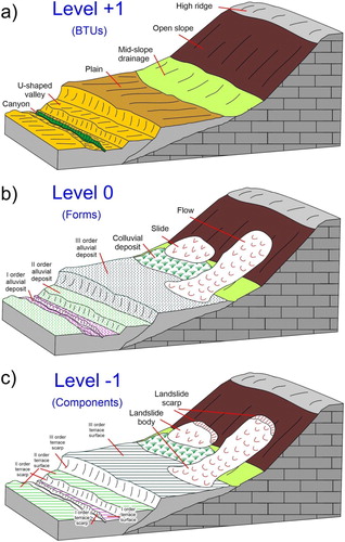
The natural, implicit characteristic of this representation is a ‘full coverage’ of the topographical surface where basic physiographic units (such as tops of the reliefs, slopes and valley floors) represent the highest hierarchical level. The novelty of this model lies particularly in the possibility of having a versatile, updatable and functional tool at different scales, depending on the use; zooming in and out in the map allows you to activate or deactivate features, details and, in general, geological and geomorphological features. Such properties make this new cartographic tool functional both for territorial planning purposes (more general) and for local applications, i.e those connected to civil engineering projects.

Taking into account the applicative purposes of the study, in the present work three different levels, only partially analogous to those of Guida et al. (2009) and Dramis et al. (2011a, 2011b), have been defined: Form (Level 0), Component (Level -1) and Basic Topographic Unit – BTU (Level +1) (Figure 1).

At the chosen reference scale (1: 10,000), the ‘Form’ (level 0) corresponds to the elements commonly mapped in traditional geomorphological maps: examples of this are landslides, river terraces, fault scarps, dunes, dolines, etc.

‘Components’ belong to a lower hierarchical level (level -1) and consist of geomorphological entities that constitute the Form and that sometimes characterize the evolutionary processes within.

A landslide, for example, may have a main scarp, some minor scarps and/or counter-slopes; the scarps, in turn, can be located within the landslide body (component itself). Other examples of components are the fluvial scarps and the flat and/or slightly inclined surfaces, which constitute the river terrace (form).

In a detailed geomorphological map, the highest level (level +1) is represented by the so-called BTUs (Basic Topographic Units), derived from medium-high-resolution DTMs (pixel resolution ranging from 30m-SRTM and 1m-LiDAR).

BTUs, in this work, have been determined using the GIS procedure developed by Weiss (2001) and based on the TPI (Topographic Position Index, as defined by Wilson & Gallant, 2000) semi-automatic landform classification. This procedure and related algorithm, improved by Jenness (2006) within the ESRI-GIS environment, has been following tested in many fields of the environmental sciences (Berking et al., 2010; Clark et al., 2012; de la Giroday et al., 2011; De Reu et al., 2013; Illés et al., 2011; Liu et al., 2009; Seif, 2014; Tağıl & Jenness, 2008; Wood et al., 2011, among others).

The TPI method measures the relative topographic position of the central point of a cell in a DTM as the difference between its elevation and the mean elevation within a pre-established neighborhood. Positive or negative values mean the cell is higher or lower respectively than the surroundings (Figure 2(a)). Weiss (2001) specified that the relationship between this value and the slope of the cell can be used to establish the position of the cell itself within a catchment and if the cell belongs to a ridge, a valley, or is part of the slope (Figure 2(b)). Following this procedure, the author developed a Slope Position Grid divided in six different categories:

Figure 2. TPI (Topographic Position Index) semi-automatic landform classification. (a) TPI at three different scale: A is very small scale it is kind of plain area; B is moderate scale is kind of small hill and C is very large scale it is a kind of valley. (b) Slope Position Classification. Weiss (2001) demonstrates one possible classification process using both TPI and slope to generate a 6-category Slope Position grid. (c) Landform Classification can be determined using 2 TPI grids at different scales.

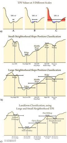
1= valley;

2= lower slope;

3= flat slope;

4= mid slope;

5= upper slopes;

6= ridges.

Using a simple algorithm (whose tool and instructions are freely downloadable with permission of the author at the address http://www.jennessent.com/arcview/tpi.htm), Jenness (2006) has following demonstrated that using two TPI grids at different scale (with large and small neighborhoods) it is possible to classify the landscape into ten morphological classes (Figure 2(c)):

1= canyons, deeply incised streams;

2= mid-slope drainages, shallow valleys;

3= upland drainages, headwaters;

4= u-shaped valleys;

5= plains;

6= open slopes;

7= upper slopes, mesas;

8= local ridges, hills in valleys;

9= mid-slope ridges, small hills in plains;

10= mountain tops, high ridges

These ‘landforms’ have been used in this works as BTUs.

The concept of full coverage, in this modern vision of geomorphological map, implies that the highest hierarchical level (BTUs) is the one that persists once the immediately lower levels are ‘turned off’. Unlike traditional geomorphological mapping, geological bedrock may not even be represented; if mapped, it must ‘persist’ (and therefore be interpreted) even below the forms and components, but over the BTUs, totally covering the study area. In this context, it is possible also to decide to keep all the original geological formations or to group them on the base of their lithotechnical behavior.

Concerning the detail of the representation of the forms and components, according to the rules of traditional cartography, the minimum unit that can be mapped to the reference scale (1: 10,000) is a polygon of 400 m² (0.04 ha) (a square of 2 mm each side), with a minimum polygon width of 20 m. Below this size, each element can be detected and arranged in an appropriate information layer that contains punctual and linear georeferenced elements.

3. Data and results

3.1. Study area

The study area falls within a predominantly high-hilly territory, located on the Adriatic side of central Italy and corresponding to the median sector of the Chienti river basin (Figure 3). The physical landscape is characterized by the presence of reliefs with gentle slopes, and relatively wide valley floors while the geological bedrock is made by alternation of mainly arenaceous-pelitic and pelitic-arenaceous levels of Messinian age, belonging to the Laga formation (Cantalamessa & Di Celma, 2004; Centamore & Deiana, 1986; Cantalamessa et al., 2002).

Figure 3. Schematic geological map of the Marche region. (1) – Main continental deposits (Pliocene-Pleistocene-Holocene); (2) – sands and conglomerates (Pliocene-Pleistocene); (3) – clays and sands (Pliocene-Pleistocene); (4) – arenaceous-marly clayey turbidites (late Miocene); (5) – limestones, marly limestones and marls (early Jurassic-Oligocene). Red star indicates the location of the study area.

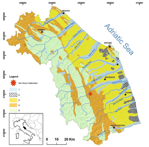
The main geomorphological features are those connected with fluvial and gravitational processes. Several orders of alluvial terraces of Quaternary age characterize the main thalweg, while small catchments, with low-order drainage systems, are directly connected to it (Buccolini et al., 2020; Gentili et al., 2017); mass movements of different type, size, state of activity and age, on the other hand, are very widespread along the slopes (Aringoli et al., 2010; Materazzi et al., 2010).

The San Rocco stream, right tributary of the Chienti River, characterizes a small catchment of around 13km2 and flows almost N-S into Le Grazie lake, one of the five artificial reservoirs built along the Chienti river itself (Figure 3). The geological bedrock, outcropping locally in correspondence of the water divides, consists, as already mentioned, of alternating sandy-pelitic and pelitic-sandy members.

Quaternary continental deposits mainly consist of medium-fine colluvial sediments and mass movements, (both active and dormant); the latter are constituted by flows (mainly) and subordinately by rotational slides and solifluctions. Concerning the land use, about 62.3% is agricultural, while the remaining part is composed of significant areas of vegetation (about 21.5%), broadleaf forests and transition shrubs (16.2%), visible only along the main incisions.

3.2. The ‘full coverage’ geomorphological mapping

The model of geomorphological map here proposed has been initially realized through a detailed field survey, carried out at the reference scale (1: 10,000), where all the geomorphological elements and the geological formations have been mapped.

The geomorphological features belong to three main categories: gravitational, fluvial and structural.

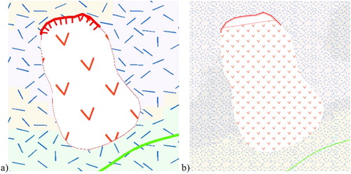
Gravitational landforms are mainly constituted by flows and slides (both translational and rotational). Flows are generally not very deep and mostly affect the colluvial deposits; rotational and translational slides can also affect the underlying marly clay bedrock, with different kinematics depending on the strata dip. State of activity and type of process have been highlighted both with a proper symbology and in the attribute table contained within the GIS database. As described in the methodology chapter, the landslide ‘form’ (level 0) has been differentiated in its two main components (body and scarp, level -1); the levels are displayed as polygons, points or polylines depending on the scale (Figure 4).

Figure 4. Example (not in scale) of ‘Levels’ of representation; (a) a Form’ landslide visible at 1: 10000 scale (Level 0); (b) another landslide subdivided in its ‘Components’ body and scarp visible at 1:1000 scale (Level – 1).

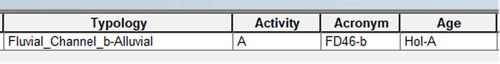
Fluvial landforms are represented by colluvial deposits, with a mainly sandy and clayey grain size, and by recent and present terraced alluvial deposits (‘Form’), locally split in two components (scarp and terrace surface). Even in this case, information about age and activity of the deposit are reported in the specific attribute table (Figure 5).

Figure 5. Example of attribute table. A (Activity): Active; Acronym: code that is given to each geomorphological typology; Hol – A: from Holocene to Actual.

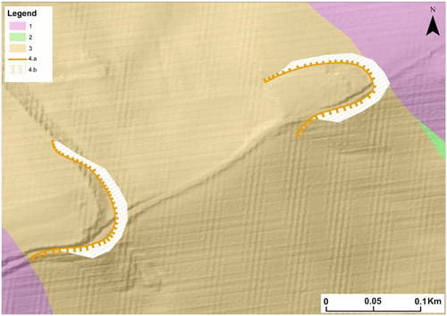
Structural landforms are finally constituted by selective erosion scarps which mark the transition between resistant levels of bedrock (arenaceous and marly) and the more erodible marly clayey and clayey ones (Figure 6).

Figure 6. Example of Selective erosion scarp. (1) lithotypes consisting of alternations (arenaceous-pelitic or pelitic-arenaceous); (2) mainly arenaceous lithotypes; (3) mainly clayey lithotypes; (4a) Selective erosion scarp (Polyline); (4b) Selective erosion scarp (Polygon).

As regards the geological bedrock, four main lithological formations have been mapped, divided into members based on mineralogical, petrographic and sedimentological characteristics.

• The Argille a Colombacci formation (FCO), divided into three members: arenaceous (FCOc), arenaceous-pelitic (FCOd) and pelitic-arenaceous (FCOe) (Messinian p.p.).

• The Laga formation (LAG), subdivided into arenaceous (LAGc), arenaceous-pelitic (LAGd) and pelitic-arenaceous (LAGe) members (Messinian p.p.); within this formation, it was also possible to differentiate the ‘Gessoso-solfifera’ member (GS), locally in clastic facies (GSa), and a volcano-clastic guide-level (a).

• The Schlier formation (SCH), consisting mainly of calcareous and clayey marls (Late Burdigalian-Lower Messinian).

The outcrops of bedrock are, however, limited, taking into account that the continental deposits cover more than 65% of the total basin area. To obtain a ‘full coverage’ of the geology of the basin, the various formations were therefore interpolated based on the stratigraphic setting, thickness and possible presence of tectonic elements. The result is shown in Figure 7(a).

Figure 7. (a) ‘Full Coverage’ Geological Map. FCOc: Argille a Colombacci formation, arenaceous member; FCOd: Argille a Colombacci formation, arenaceous-pelitic member; FCOe: Argille a Colombacci formation, pelitic-arenaceous member; GS: Gessoso-solfifera member, GSa: clastic facies; LAG3c: Laga formation, arenaceous member; LAG3d: Laga formation, arenaceous- pelitic member; LAG3e: Laga formation, pelitic- arenaceous member; SCH: Schlier formation; a: volcano-clastic guide-level; (b) Lithotechnical Map. (1) lithotypes consisting of alternations (arenaceous-pelitic or pelitic-arenaceous); (2) mainly arenaceous lithotypes; (3) mainly clayey lithotypes.

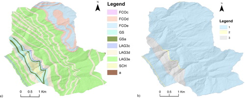
Taking into account the fundamental objectives of a geomorphological map, an additional information layer was therefore created where the aforementioned formations were grouped into three classes based only on their lithotechnical characters:

1. mainly clayey lithotypes;

2. mainly arenaceous lithotypes;

3. lithotypes consisting of alternations (arenaceous-pelitic or pelitic-arenaceous).

The result is shown in Figure 7(b).

As for the definition of the BTUs, the method proposed by Weiss (2001), following adapted by Jenness (2006) for the ESRI-Enterprise (version 10.7) GIS environment was subsequently used. Through an iterative procedure, the TPI neighborhoods (small and large) have been varied to find the best correspondence between the ‘landforms’ obtained from the method and the real morphologies visible on a DEM.

The method was tested on three DTMs with different details, to also check for the presence of a possible relationship between neighborhoods and pixel resolution.

More specifically, the following DTMs were used:

• SRTM 1 Arc Second Global (30 m cell-size);

• TINITALY (10 m cell-size);

• LiDAR (1 m cell-size).

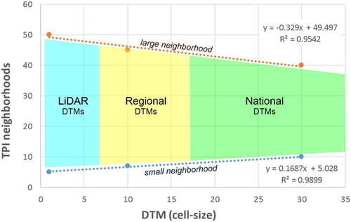
The most satisfactory results were obtained using the following neighborhood combinations

1. SRTM (small neighborhood = 10m; large neighborhood = 40m);

2. TINITALY (small neighborhood = 7m; large neighborhood = 45m);

3. LiDAR (small neighborhood = 5m; large neighborhood = 50m).

It is interesting to note that there is an almost linear relationship between the intervals (small and large neighborhoods) and the resolution of the DTM itself; to an increase in resolution generally corresponds an increase in the interval (Figure 8).

Figure 8. Relationships between neighborhood intervals and DTM cell-size.

The results of the various elaborations are shown in Figure 9(a–c).

Figure 9. Landform Classification Map. (a) SRTM (small neighborhood = 10 m; large neighborhood = 40 m); (b)TINITALY (small neighborhood = 7 m; large neighborhood = 45 m); (c) LiDAR (small neighborhood = 5 m; large neighborhood = 50 m); In black the Study Area.

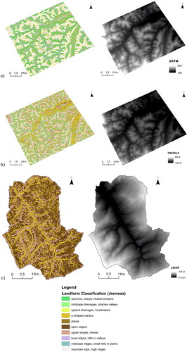
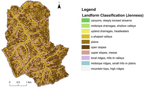
Considering the size of the study area and the correspondence obtained, it was, therefore, decided to use as BTUs the ‘landforms’ obtained by processing the DTM-LiDAR and the combination indicated in Figure 9c (Figure 10).

Figure 10. The BTUs Map for San Rocco Stream Basin.

4. Discussion

The methodology proposed, whose application example can be consulted interactively at the address https://arcg.is/1yOnae certainly brings significant advantages compared to a traditional cartography (Main Map).

• First of all, the use of a GIS system and a database of georeferenced attributes makes this cartographic tool extremely dynamic and able for storing and updating multiple types of information; these can be following filterable on demand.

• The subdivision into hierarchical levels allows a more rational use of the represented geomorphological processes and landforms; a greater detail is fundamental for design purposes, while a lesser detail is more functional for territorial planning studies or hydro-geomorphological risk assessment.

• Hierarchical levels of both upper and lower rank can be increased in number according to the scale of the map. Upper ranks may include complex landforms or groups of landforms (Deep Seated Gravitational Slope Deformations, fields of dolines, etc.) up to morphotectonic systems or more general physiographic domains, significant at the regional or continental levels respectively; a lower rank allows to characterize minor elements, nevertheless important for a complete characterization of the active processes in a specific area (alluvial fan channels, coastal cliff notches, etc.).

• A ‘full coverage’ finally allows us to have topographical, geological, geomorphological information in every point of the map, regardless of the scale of visualization. Compared to a traditional mapping, as well as in reality, it is possible to find a ‘bedrock’ (geological or simply morphological) under each geomorphological landform.

The limits of the method, on the other hand, are essentially linked to two crucial aspects, both of which can be traced back to the definition of the BTUs.

• As mentioned in the introduction chapter, such a methodology should be applicable on a national scale. If on the one hand, however, the choice of a unique TPI-neighborhood interval is easily achievable, this is not for the DTM. If the purpose is a high-scale geomorphological map, no complete coverage of the LiDAR topographic data in Italy is available; besides, the choice of the most suitable method for the landform classification does not always seem applicable to all contexts.

• The second aspect is linked to the need to have a correspondence between ‘landforms’ defined with automatic procedures and geomorphological landforms mapped through field surveys (i.e. fluvial terrace surface coinciding only with a ‘plain’ landform or landslides corresponding to ‘open slope’). Notwithstanding that the expert judgment of the geomorphologist remains fundamental for a correct recognition and delimitation of geomorphological landforms and processes, a strong debate remains between those believing that the above features should be ‘adapted’ to the ‘automatic landforms’ (Dramis et al., 2011b) and those who consider indispensable the field survey constraint (Klimaszewski, 1982). In our opinion, this dispute could be overcome considering such correspondence, not a binding element; a landslide can be part of two distinct ‘landforms’ as well as a fluvial terrace surface could be partially contained within ‘u-shaped valleys’ or ‘plains’.

5. Conclusions

A ‘full coverage’ geomorphological mapping, as highlighted in this paper, can represent the synthesis between two models of cartography that the scientific and the professional world have so far adapted only to their needs. In particular, the hierarchical model proposed here allows us to reconcile the needs of those who ask for high detail and application-type information and those who need to keep canons and rules of an official cartography, structured at a national scale.

The advantages of such an approach are undoubtedly:

• The use of a mapping system structured and managed within a Geographical Information System (GIS) that allows to work for hierarchical levels and nested entities, thus representing all the elements constituting a typical geomorphological ‘form’ (landslide, alluvial terrace, etc.).

  • The possibility to collect a lot of information and to organize and display them in different detail, depending on the use and scale of representation.

  • The possibility of having a ‘dynamic’ cartography, suitable to be updated and implemented in the light of the new information acquired. Following, different thematic maps can be easily derived for practical uses.

The main problem, on the other hand, is essentially related to the definition of the BTUs: as a high-resolution DTM (i.e. LiDAR) is not often available for the whole national territory, it becomes very difficult to define this level within an official cartography.

Software and basic DTMs

All data processing necessary to produce the map was performed using ESRI-ArcMap (version 10.7). The interactive map was created using ESRI-Enterprise 10.7 and ArcGIS Online. The figures in the document were created using CorelDraw Home&Student 2019.

Concerning the DTMs all three have been collected from the following sources:

• SRTM 1 Arc Second Global (30 m cell-size) freely downloadable from USGS site (https://earthexplorer.usgs.gov/);

• TINITALY (10 m cell-size), freely downloadable at the link http://tinitaly.pi.ingv.it/Download_Area2.html (Tarquini et al., 2007; Tarquini & Nannipieri, 2017);

• LiDAR (1 m cell-size), courtesy of the Italian ‘Ministry of the Environment and the Protection of the Territory and the Sea’ (http://www.pcn.minambiente.it).

Acknowledgements

The Authors wish to thank the expert reviewers for the useful suggestions which significantly improved the final version of the manuscript.

Disclosure statement

No potential conflict of interest was reported by the author(s).

References

- Abdulrahman, A. I. (2020). Landform clarification using automated Techniques in Geographical Information systems.
- Aringoli, D., Gentili, B., Materazzi, M., & Pambianchi, G. (2010). Mass movements in Adriatic central Italy: Activation and evolutive control factors. In E. D. Werner, & H. P. Friedman (Eds.), Landslides: Causes, types and effects (pp. 1–71). Nova Science Publishers, Inc.
- Berking, J., Beckers, B., & Schütt, B. (2010). Runoff in two semi-arid watersheds in a geoarcheological context: A case study of naga, Sudan, and resafa, Syria. Geoarchaeology, 25(6), 815–836. https://doi.org/10.1002/gea.20333
- Bishop, M. P., James, L. A., Shroder Jr.J. F., & Walsh, S. J. (2012). Geospatial technologies and digital geomorphological mapping: Concepts, issues and research. Geomorphology, 137(1), 5–26. https://doi.org/10.1016/j.geomorph.2011.06.027
- Brunsden, D., Doornkamp, J. C., Fookes, P. G., Jones, D. K. C., & Kelly, J. M. H. (1975). Large scale geomorphological mapping and highway engineering design. Quarterly Journal of Engineering Geology and Hydrogeology, 8(4), 227–253. https://doi.org/10.1144/GSL.QJEG.1975.008.04.01
- Buccolini, M., Bufalini, M., Coco, L., Materazzi, M., & Piacentini, T. (2020). Small catchments evolution on clayey hilly landscapes in central Apennines and northern sicily (Italy) since the late pleistocene. Geomorphology, 363 107206, https://doi.org/10.1016/j.geomorph.2020.107206
- Butler, D. R., & Walsh, S. J. (1998). The application of remote sensing and geographic information systems in the study of geomorphology: An introduction. Geomorphology, 21(3-4), 179–181. https://doi.org/10.1016/S0169-555X(97)00056-1
- Cantalamessa, G., Centamore, E., Didaskalou, P., Micarelli, A., Napoleone, G., & Potetti, M. (2002). Elementi di correlazione nella successione marina plio-pleistocenica del bacino periadriatico marchigiano. Studi Geol. Camerti, Nuova Serie, 1(2002), 33–49. (in italian).
- Cantalamessa, G., & Di Celma, C. (2004). Sequence response to syndepositional regional uplift: Insights from high-resolution sequence stratigraphy of late early Pleistocene strata, periadriatic basin, central Italy. Sedimentary Geology, 164(3-4), 283–309. https://doi.org/10.1016/j.sedgeo.2003.11.003
- Canuti, P., Focardi, P., Garzonio, C. A., Rodolfi, G., & Vannocci, P. (1987). Slope stability mapping in Tuscany, Italy. International Geomorphology, 1, 231–240. John Wiley & Sons.
- Centamore, E., & Deiana, G. (1986). La Geologia delle Marche. Studi Geologici Camerti, vol.spec., 1–145 (in Italian).
- Clark, J. T., Fei, S., Liang, L., & Rieske, L. K. (2012). Mapping eastern hemlock: Comparing classification techniques to evaluate susceptibility of a fragmented and valued resource to an exotic invader, the hemlock woolly adelgid. Forest Ecology and Management, 266, 216–222. https://doi.org/10.1016/j.foreco.2011.11.030
- De Graaff, L. W. S., De Jong, M. G. G., Rupke, J., & Verhofstad, J. (1987). A geomorphological mapping system at scale 1: 10,000 for mountainous areas. Zeitschrift für Geomorphologie, 31(2), 229–242.
- de la Giroday, H.-M., Carroll, A., Lindgren, B., & Aukema, B. (2011). Incoming! Association of landscape features with dispersing mountain pine beetle populations during a range expansion event in western Canada. Landscape Ecology, 26(8), 1097–1110. https://doi.org/10.1007/s10980-011-9628-9
- De Reu, J., Bourgeois, J., Bats, M., Zwertvaegher, A., Gelorini, V., De Smedt, P., … Van Meirvenne, M. (2013). Application of the topographic position index to heterogeneous landscapes. Geomorphology, 186, 39–49. https://doi.org/10.1016/j.geomorph.2012.12.015
- Directive INSPIRE. (2007). Directive 2007/2/EC of the European Parliament and of the Council of 14 March 2007 establishing an Infrastructure for Spatial Information in the European Community (INSPIRE). Published in the official Journal on the 25th April. http://eur-lex.europa.eu/JOHtml.do?uri=OJ:L:2007:108:SOM:EN:HTML
- Dramis, F., Giuda, D., Cestari, A., Siervo, V., & Palmieri, V. (2011b). Dalla cartografia geomorfologica al sistema cartografico geomorfologico: Metodologie, procedure e applicazioni. Geologia Tecnica e Ambientale, 3(3), 10–25.
- Dramis, F., Guida, D., & Cestari, A. (2011a). Geomorphological Mapping: Methods and Applications. developments in earth Surface Processes Nature and aims of geomorphological mapping. Smith m.j., Paron P. & GriFFithS j.S. (eds.) 15, 39–73.
- Gentili, B., Pambianchi, G., Aringoli, D., Materazzi, M., & Giacopetti, M. (2017). Pliocene-Pleistocene geomorphological evolution of the Adriatic side of central Italy. Geologica Carpathica, 68(1), 6–18. https://doi.org/10.1515/geoca-2017-0001
- Guida, D., De Pippo, T., Cestari, A., Siervo, V., & Valente, A. (2009). Applications of the hierarchic GIS-based geomorphological mapping system. Proceedings of the 3rd AIGEO National Conference, Modena, Italy (pp. 13–18).
- Gustavsson, M., Kolstrup, E., & Seijmonsbergen, A. C. (2006). A new symbol-and-GIS based detailed geomorphological mapping system: Renewal of a scientific discipline for understanding landscape development. Geomorphology, 77(1-2), 90–111. https://doi.org/10.1016/j.geomorph.2006.01.026
- Hayden, R. S. (1986). Geomorphological mapping. In N. M. Short & R. W. Blair Jr. (Eds.), Geomorphology from space (pp. 637–656). NASA.
- Illés, G., Kovács, G., & Heil, B. (2011). Comparing and evaluating digital soil mapping methods in a Hungarian forest reserve. Canadian Journal of Soil Science, 91(4), 615–626. https://doi.org/10.4141/cjss2010-007
- ISPRA. (2018). Aggiornamento ed integrazioni delle Linee Guida della Carta Geomorfologica d'Italia alla Scala 1:50000. ISPRA-Serv.Geol.Italia, Quaderni Serie III, Vol. 13, fascicolo 1. 2018:93 pp.
- Jenness, J. (2006). Topographic Position Index (tpi_jen.avx) extension for ArcView 3.x, v. 1.3a. Jenness Enterprises. http://www.jennessent.com/arcview/tpi.htm
- Kienholz, H. (1978). Maps of Geomorphology and natural hazards of grindelwald, Switzerland: Scale 1: 10,000∗. Arctic and Alpine Research, 10(2), 168–184. https://doi.org/10.2307/1550751
- Klimaszewski, M. (1982). Detailed geomorphological maps. ITC Journal, 3, 265–271.
- Klimaszewski, M. (1990). Thirty years of detailed geomorphological mapping. Geographia Polonica, 58, 11–18.
- Liu, M., Hu, Y., Chang, Y., He, X., & Zhang, W. (2009). Land use and land cover change analysis and prediction in the upper reaches of the minjiang river, China. Environmental Management, 43(5), 899–907. https://doi.org/10.1007/s00267-008-9263-7
- Materazzi, M., Gentili, B., Aringoli, D., Farabollini, P., & Pambianchi, G. (2010). Elements of slope and fluvial dynamics as evidence of late holocene climatic fluctuations in the central adriatic sector, Italy. Geogr. Fis. e Din. Quat, 33, 193–204.
- Seif, A. (2014). Using topography position index for landform classification (case study: Grain mountain). Bulletin of Environment, Pharmacology and Life Sciences, 3(11), 2277–1808.
- Smith, M. J., Paron, P., & Griffiths, J. S. (2011). Geomorphological mapping: Methods and applications. In M. J. Smith, P. Paron, & J. S. Griffiths (Eds.), Developments in Earth surface processes, vol. 15, British society for geomorphology (661pp.). Elsevier Science.
- Tağıl, Ş, & Jenness, J. (2008). GIS-based automated landform classification and topographic, land cover and geologic attributes of landforms around the Yazoren Polje, Turkey.
- Tarquini, S., Isola, I., Favalli, M., Mazzarini, F., Bisson, M., Pareschi, M. T., & Boschi, E. (2007). TINITALY/01: a new triangular irregular network of Italy. Annals of Geophysics.
- Tarquini, S., & Nannipieri, L. (2017). The 10 m-resolution TINITALY DEM as a trans-disciplinary basis for the analysis of the Italian territory: Current trends and new perspectives. Geomorphology, 281, 108–115. https://doi.org/10.1016/j.geomorph.2016.12.022
- Ten Cate, J. A. (1990). Sea-level rise and geomorphological mapping. Geographia Polonica, 58, 19–39.
- Van Westen, C. J., Rengers, N., & Soeters, R. (2003). Use of geomorphological information in indirect landslide susceptibility assessment. Natural Hazards, 30(3), 399–419. https://doi.org/10.1023/B:NHAZ.0000007097.42735.9e
- Weiss, A. (2001, July 9–13). Topographic position and landforms analysis. Poster presentation, ESRI user conference, San Diego, CA (Vol. 200).
- Wilson, J. P., & Gallant, J. C. (2000). Terrain analysis: Principles and applications (479pp.). John Wiles & Sons.
- Wood, S. W., Murphy, B. P., & Bowman, D. M. (2011). Firescape ecology: How topography determines the contrasting distribution of fire and rain forest in the south-west of the tasmanian wilderness world heritage area. Journal of Biogeography, 38(9), 1807–1820. https://doi.org/10.1111/j.1365-2699.2011.02524.x