Spatial distribution of criminal events in Lithuania in 2015–2019

ABSTRACT

The presented map poster represents statistics for 3.46 million events reported to the police in Lithuania in 2015–2019. For eight types of events (violent crime, theft, property crime, economic crime, infringement of public policy, drug-related crime, traffic accidents, various other events), two maps at a scale of 1:3,000,000 are presented. They demonstrate the values of location quotient and the main insights into the dynamics of crime over the five-year timeframe covered by the project. Two maps at scale 1:2,000,000 show the distribution of five types of events that are directly related to the safety of persons – totalling 1.67 million records. One of the larger scale maps depicts the relative crime rate, separately for densely and sparsely populated areas. The second map shows the relative crime risk surface. The maps enable a visual analysis of the most problematic areas in Lithuania and can enable deeper further investigation.

KEYWORDS:

• Crime
• maps
• safety
• spatial distribution
• dynamics
• relative risk

1. Introduction

Only since about 2011 have spatial methods been commonly applied to the analysis of crime in Lithuania. During the last decade, several studies on the geographic distribution of crime have been published, but they were still either very general or focused on crime in particular small expanses of territory, mainly big cities or parts of cities. The possibilities of more extensive analysis were limited because the national and municipal datasets on crime had internal inconsistencies and were not always comparable with each other. Since 2015, the dataset of the departmental Register of Events Registered by the Police (hereinafter RERP) that covers the entire territory of Lithuania has been accessible to researchers. The period of 2016–2020 be characterized by the relative stability of the situation and a slow but constant decrease of crime in general. However, the situation was not the same in different parts of the country.

The principal aim of this research is to examine the distribution of crime-related event data over the territory of Lithuania in order to identify and visualize the trends and spatial patterns of change.

The main research question centres upon regional peculiarities of the distribution of crime that cannot be accounted for by density of population or level of urbanization. The mapping and spatial analysis of crime data is aimed at determining:

1. irregularities in the distribution of the relative crime rate, particularly of crime in open space over the territory of Lithuania;

2. structural differences of crime in urban and rural areas;

3. peculiarities of temporal trends, focusing on the areas where growth of relative crime rates is clearly expressed.

The series of maps represent the applied results of this research. For the poster presented, we have selected the results of analysis that appear most applicable for visual interpretation. Two main maps represent the five types of events that are directly related to crime. With the maps presented we only draw attention to irregularities in the distribution of crime, without attempting to explain the reasons for these irregularities or to forecast trends, those being tasks for criminologists. Still, we believe that the maps have practical value to crime researchers and policy makers in a variety of possible ways including deeper spatial insights, as well as comparison and development of priorities for crime prevention – it was demonstrated in earlier study of one Lithuanian city (Acus et al., 2018). The maps can also be used for comparison of the general distribution of crime and specific insights (Ceccato, 2007, 2009; Ceccato & Oberwittler, 2008; Sypion-Dutkowska & Leitner, 2017) in countries that are geopolitically similar to Lithuania, notably the Baltic states and other states in the former Eastern Bloc that joined the European Union in the twenty-first century.

2. Background and related works

Methods of crime mapping have been applied and developed for more than 200 years. Hundreds of research papers, monographs and textbooks have been published on different aspects of the topic – from particular methods of crime mapping (Boba, 2005; Brantingham & Brantingham, 1981; Brantingham & Brantingham, 1995; Chainey & Ratcliffe, 2005; Ghosh et al., 2012; Leitner, 2013; McCune, 2010; Walker & Dwarve, 2018) to advanced GIS analysis and modelling of crime hot spots (Brown, 1982; Eck et al., 2005; Frank et al., 2011), software tools and web maps (Gorr et al., 2018; Leong & Chan, 2013; Levine, 2015). Nevertheless, the appropriate visualization of crime in a particular socio-cultural context remains a challenge. Sophisticated theoretical models and assumptions that have been applied with varying level of success in large countries like the US (Anselin et al., 2000; Boba-Santos, 2017; Hart & Lersch, 2015), Canada (Andresen, 2007; Savoie, 2008), UK or Australia (Carcach & Muscat, 2002; Chainey, 2014) would not necessarily work well for Lithuania – a small country with a highly specific political and socio-demographic set of features. The country is a member of the European Union, but is also post-Soviet, located at the eastern periphery of the EU/NATO area of Europe, and still in the process of a societal shift to Western democratic structures.

Reliable analytical insights and forecasts can only be set out based on national data. Unfortunately, there are not so many studies on spatial distribution of crime in the Baltic states that are similar to Lithuania in this sense; the existing studies are mostly descriptive (Ceccato, 2007, 2008, 2009). In our previous papers (Beconytė et al., 2020 Vasiliauskas & Beconytė, 2016;) we provided a brief summary of geographic crime research in Lithuania. The main conclusion has not changed, and that is for one reason, namely that since the beginning of professional crime mapping ca. 2010, analytical crime maps of Lithuania were only available for the major urban areas. The only crime map orientated to a cartographic communication of crime was designed for the capital Vilnius (Vasiliauskas & Beconytė, 2016). In the most recent publication (Beconytė et al., 2020), we introduced two maps that cover the entire territory of Lithuania: relative risk surfaces for total and open space crime. Further investigations resulted in an improved relative risk map that is presented in the present paper. The methods used for this map are based on the insights on density mapping of data that are not normally distributed (Bithell, 1991; Kiessé, 2017; Kokonendji & Somé, 2015; Scott, 2015).

Kernel density mapping is one of the methods of visualization for intensity function for spatial point process. The bivariate radial-symmetric kernel density estimation (KDE) with common function $\hat{f}(x,y)$ without edge correction at a location $x,y$ is $\hat{f}(x,y)={\displaystyle \frac{1}{n{h}^2}\sum _{\mathrm{i}=1}^{n}K\left({\displaystyle \frac{d_{(x,y),i}}{h}}\right)}$where x and y are two-dimensional (2D) spatial co-ordinates within а bounded study region; $K$ is a 2D, second-order, zero-centred, radially symmetric continuous bimodal fixed kernel function; $d_{(x,y),i}$ is the Euclidean distance between event-point $i$ and location $(x,y)$; $h$ is the kernel bandwidth that is scaled equally in all directions or the radius of a circular kernel (Silverman, 1986).

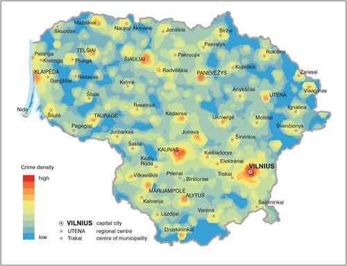
A series of experiments on kernel estimations for the crime count data of Lithuania has been conducted. They include a selection of different bandwidths (Abramson, 1982; Davies & Baddeley, 2018; Davies & Lawson, 2019; Hazelton, 2008; Kelsall & Diggle, 1995), derivation of kernel functions (Davies et al., 2016), calculation of kernel surfaces and calculation of point process residual (Loader, 1999) to compare and validate the results. Estimated bivariate radial-symmetric kernel surface with an isotropic adaptive bandwidth (with range of 150–3500 m) is shown in Figure 1 – low and high values are represented by blue and red colouring respectively. The occurrences of crime are not uniformly distributed over the space covered; they are, rather, concentrated in populated places. In areas with higher population density more crime events can be expected, and corresponding clusters do indeed appear in the towns.

Figure 1. Estimated crime density for the five main types of events, for 2015–2019.

Map of Lithuania show crime density as a surface, low to high values represented by diverging colour scale.

The common method that allows for adjusting kernel density for an underlying covariate (in our case population) is based on the spatial relative risk or density-ratio function that was first proposed by Bithell (1991).

The location quotient coefficient (LQ) was first proposed and applied to location analysis in regional economics and regional planning (Haggett et al., 1980). Its application for crime mapping has been demonstrated by Brantingham and Brantingham (1995, 1998). Although the LQ does not represent the crime rate, it is useful as an indicator of a disproportionate share of a particular type of crime in a territorial unit. Thus, LQ maps complement crime rate maps and facilitate understanding of the patterns of different types of crime (Andresen et al., 2009; Ratcliffe & Rengert, 2008).

3. The dataset

The RERP dataset that was used in the research contains 3.46 million records of events reported to the police of Lithuania in 2015–2019.

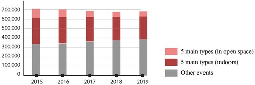
In the RERP, there are seven main types of events: violent crime (homicide, murder, assault, manslaughter, sexual assault, rape, robbery, abduction, harassment), thefts, property crime (criminal damage), economic offence (forgery, tax evasion, trade diversions, handling contraband and counterfeit goods), infringement of public policy (breach of the peace, illicit consumption of alcohol), traffic accidents and various other incidents (drug related crime, arrests, suspicious persons or things, aid for special services, lost and found documents, activation of burglary alarm systems etc.). We have separately analysed drug-related crime that is classified as ‘various other’ in RERP, but is important as a direct threat to public safety. Thus, five types of events relate directly to the safety of persons: violent crime, theft, property crime, infringement of public policy and drug-related crime – total 1.67 million event points. We refer to these below as the ‘five main types’ or ‘crime events’. The total number of the events belonging to these five types gradually decreased from 381,694 in 2015–298,901 in 2019. The decrease in the number of events in open space from 2015 to 2019 (45%) was relatively much larger than of those indoors (14%) – this may be due to better prevention of crime in open spaces (Figure 2).

Figure 2. Dynamics of crime events in 2015–2019.

Column chart representing absolute numbers and shares of registered events in 2015, 2016, 2017, 2018 and 2019: five main types of events in open spaces and indoors, and other events.

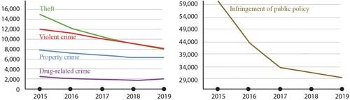
The dynamics of each of the five main types are shown in Figure 3. The numbers for public nuisance events are several times higher than of the other types, thus they are shown in a separate chart.

Figure 3. Dynamics of crime events in open space, number of incidents.

Graphs representing absolute numbers of events by type in 2015, 2016, 2017, 2018 and 2019.

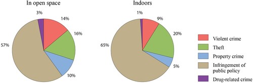
The structure of crime in open space and indoors is different (Figure 4) – the share of the four more serious violations (violent crime, theft, property crime and drug-related crime) is much larger in open space (43%) than indoors (35%).

Figure 4. Structure of crime events, average for 2015–2019.

Two pie charts representing structure of crime in Lithuania in open space and indoors.

The latest census dataset for Lithuania is for 2011. Since then, population counts changed (decreased in rural areas) due to urban migration and other causes. A new population dataset that was used for crime rate estimates was published by Statistics of Lithuania in 2020 (Population and Housing Census, 2020). Its findings have been estimated from official registers, taking migration and other important elements into account. Only when the new census data become available in 2021 will it be possible to evaluate the accuracy of the estimates provided, but we consider it more applicable for our purposes than the 10-year-old census dataset. Estimated population data were aggregated into 25 km² hexagonal cells for the maps of LQ and the dynamics of crime and into a regular grid of 586,952 points (one point for five people) for kernel density and relative risk mapping.

Reference base data of the Lithuanian part of the EuroRegionalMap dataset at scale 1: 250 000 was generalized and used for topographic background information: shoreline, towns and state boundaries.

3.1. Aggregation of data

A grid of 25 km² hexagonal cells covering the entire territory of Lithuania was generated. The grid was designed to more or less optimally cover the urban areas. Based on our previous research, we considered this size appropriate and convenient for the representation and visual analysis of crime in the country. The grid was used for the aggregation of crime events and estimated population data. To minimize the impact of possible population estimation errors and to avoid possible misinterpretations of crime rate, the cells with a population smaller than 100 (less than four people/km²) were excluded from the calculations and have not been represented on the maps (total 552 cells, 20% of all cells). For a more precise representation of crime rate, the cells with population larger than 2500 (more than 100 people/km²) have been divided into sub-cells of 8.3 km² each.

3.2. Events in very sparsely populated cells

There were 552 cells that were excluded because these were very sparsely populated. Of these, 542 had fewer than 10 annual crime events on average, and the remaining 10 had fewer than 22.5 crimes on average.

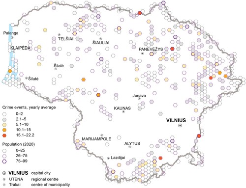
Five cells have slightly higher occurrence of crime (red cells in Figure 5) that are mainly due to infringements of public policy in open space. One such cell is the beach area of the popular resort Neringa (no residents, but on average 13 events per year). The cell with highest average annual number of crime events is at the state border crossing point (95 residents, on average 22.2 events per year, practically none in open space). Several other, still unexplained, are the rural areas of eastern Lithuania. Generally, only about 16% of all events reported in very sparsely populated cells occurred in open space.

Figure 5. Crime events in very sparsely populated cells (average for 2015–2019).

Map of Lithuania with hexagonal cells for very sparsely populated areas, the average yearly number of events, represented by background colour, is mainly less than five.

4. The method

For cartographic representation, we have selected the following spatial aspects of crime:

1. Crime rate for the five main types of events that exhibit strong correlation with population – violent crime, theft, property crime, infringement of public policy and drug-related crime;

2. Relative risk for the five main types of events;

3. Location quotient for each of the eight types of events;

4. Dynamics, emphasizing locations of persistent significant growth (or decrease) of rate for of the eight types of events;

5. Location quotient and dynamics for the five main types of events that occurred in open space.

4.1. Crime rate map

The map shows the annual average number of events of the five main types per 1,000 population. Separate intervals and colour schemes are constructed for densely populated (more than 100 people/km²) and sparsely populated (4–100 people/km²) cells – using yellow and blue graduated colour schemes, respectively. Densely populated original cells have been divided into three diamond-shaped sub-cells each.

4.2. Location quotient maps

The values of LQ have been calculated for each type of events and represented on eight separate maps at scale 1:3,000,000 each. Based on the total amount of crime in 2015–2019, they show the share of particular crime type in the cell in comparison to the cell’s share of the total occurrence of crime: $L{Q}_{ij}=\left({\displaystyle \frac{c_{ij}}{C_j}}\right)/{\displaystyle \frac{{\sum }_{j=1}^N{c}_{ij}}{{\sum }_{j=1}^N{C}_j})}$where c_ij is the number of events of type i in cell j, C_j is the number of events of all types in cell j, N is the number of cells in the country.

If LQ > 1, this indicates a higher spatial concentration of particular crime type in a given cell, compared to the average share of each cell. If LQ < 1, the particular crime type has a share less than is found throughout Lithuania. On the maps, disproportionally high LQ values (more than 1.5) are represented by a colour specific to the particular event type. They do not indicate that this particular type of crime prevails in the given area – it just manifests there more strongly than in the country in general. Low values (less than 0.75) are shown in the same light blue colour on all maps in the series.

The cells in which no events were reported have not been represented on the corresponding location quotient maps. Only those intervals of LQ values that are present on the map, are shown in its legend. Clusters of densely populated cells are marked by a thicker contour line.

4.3. Maps of event dynamics

The relative number of events is not normally distributed. Deeper analysis of temporal data has revealed that dynamics have been different every year for each type of event. Thus, simple visualizations of dynamics using standard tools can be misleading. We applied an original algorithm that considers annual differences in relative event rate and the overall trend. It allows delineation of steady and substantial positive and negative trends.

The annual difference of the relative event rate for each cell C_ij was classified as:

1. substantial increase (SI), if the value is larger than the median value for the positive changes for the corresponding year j (2016, 2017, 2018 and 2019);

2. increase (I) if the value is in the second quartile of the positive changes;

3. stability (S) if the value is in the first quartiles of the positive and negative changes;

4. decrease (D) if the value is in the second quartile of the negative changes;

5. substantial decrease (SD), if the value is lower than the median value for the negative changes.

A five-year trend C_iT was assigned based on the same statistics, but was actually estimated for the difference of the relative event rate between 2019 and 2015.

The general type of dynamics CT_i was determined combining the values of C_ij and C_iT as shown in the Table 1.

Table 1. Estimation of types of dynamics for the cell C_i.

CiT	Values of Cij in the set for 2015–2019	Type of dynamics CTi	Symbol
SI	Only SI and I	SI (substantial increase)
SI	SI, I, S; up to one D	I (increase)
I	Up to two S; no SD, no D
I or S or D	I, S, D; no SI, no SD	S (stability)
Any	Both SI and SD; any other	O (ocillation)
D	Up to two S, no SI, no I	D (decrease)
SD	SD, D, S; up to one I
SD	Only SD and D	SD (substantial decrease)

The values of C_iT for different types of events have been represented on eight separate maps at scale 1:3,000,000 each.

The cells for which no events were reported have not been represented on the corresponding maps. Only those types of dynamics that are present on the map, are shown in its legend. Clusters of densely populated cells are highlighted by a thicker contour line.

4.4. Crime in open space

A separate LQ map and map of dynamics have been designed for the five main types of events that occurred in open space in 2015–2019. These maps are compiled at a smaller scale – 1:4,000,000 each.

The cells for which no events were reported have not been represented on the corresponding maps. As on the other maps, only those LQ values and only those types of dynamics that are present on maps, are shown in their legends. Clusters of densely populated cells are highlighted by a thicker contour line.

4.5. Relative risk surface

The relative crime risk surface portrays the estimated probabilities of crime events across the country. The spatial relative risk function can be employed for handling the heterogeneity in the distribution of the data. If both the kernel bivariate densities of crime events $K_e(\cdot )$ and the population at risk $K_p(\cdot )$ are estimated through their own KDE processes, then the joint spatial relative risk function $\hat{r}(x,y)$ can be expressed as the ratio of densities describing respectively the spatial distribution of crime events and of the population at risk: $\hat{r}(x,y)={\displaystyle \frac{\widehat{f_e}(x,y)}{\widehat{f_p}(x,y)}}$where, the $\widehat{f_e}$ and $\widehat{f_p}$ are the kernel functions.

Jointly optimal fixed bandwidths for the spatial relative risk function were estimated using the least-squares cross-validated selector. The estimated jointly optimal fixed spatial bandwidths for the Gaussian KDE relative risk function were 1,280 and 680 m for the selectors based on mean integrated squared error MISE (Kelsall & Diggle, 1995) and on a weighted MISE (Hazelton, 2008) respectively.

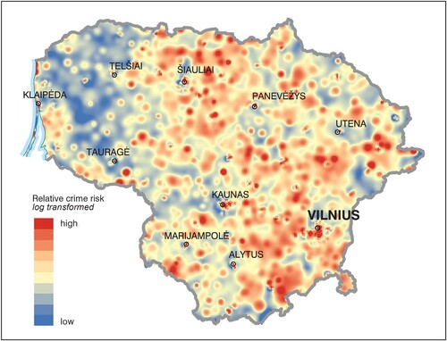
Symmetric pooled adaptive Gaussian KDE relative risk function with global and pilot bandwidths at 680 metres was used to generate a risk surface. The relative risk surface is represented in Figure 6. Areas of average risk density where log-transformed relative risk equals to zero, i.e. where KDEs of crime events and population at risk are equal, are represented in yellow. Peaks (red colour) in the surface where log-transformed relative risk values are larger than zero show a higher localized concentration of crime relative to population density, in many cases in suburban areas. The depressions (blue colour) where log-transformed relative risk is less than zero represent territories with a relatively low crime rate.

Figure 6. Estimated log-transformed relative risk surface, 2015–2019.

Map of Lithuania showing surface of relative risk of crime, represented by diverging colour scale.

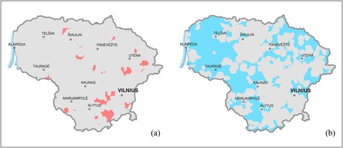
Figure 7 shows asymptotic $p$-value surfaces with tolerance areas from an upper-tailed test and a lower-tailed test at significant 5% thresholds of elevated (a) and reduced (b) risk respectively. The pointwise p-value surfaces were computed based on asymptotic theory of adaptive kernel-smoothed relative risk surfaces described by Davies and Baddeley (2018). The highlighted areas represent regions of potentially anomalous crime activity with significantly increased and decreased crime risk relative to the background population density. They match regions of extreme values of relative risk surface (Figure 6). High relative risk areas are of interest because the reasons for these anomalies are unknown and require further research. In order to formulate strong hypotheses, much deeper investigation including victimization surveys in those areas must be conducted.

Figure 7. (a) high relative risk areas (p ≤ .05); (b) low relative risk areas (p ≤ .05).

Two schematic maps of Lithuania showing high relative risk areas mainly in south-eastern part and low relative risk areas mainly in western part.

5. Discussion and concluding remarks

The series of crime maps and charts on the main poster reveal several peculiarities of the spatial distribution and dynamics of crime in Lithuania. Together with open aggregated spatial dataset, the maps can be used by the police and municipal administrations for development of more efficient crime prevention programme and by criminologists for further detailed research.

The overall pattern of events is not unexpected. Population is a very good predictor of event count and variations are moderate. However, there are differences in structure and dynamics of crime in sparsely and densely populated rural areas that yet have to be investigated. At the moment, it would be difficult to explain the pattern of highest relative crime risk in these areas.

A substantial decrease in the number of reported events has been observed from 2015 to 2019, mainly due to a decrease in public nuisances in open spaces (Figures 2 and 3), but also due to a decrease in the other types. That could have also been expected in light of an improving economic and social situation and, possibly, due to the sharp decrease in consumption of alcohol. We believe that the reasons of a drop in property crime and of increase in violent crime reflect the general patterns described in an earlier study of Western Europe by Aebi and Linde (2010). In Lithuania, each event type has its own pattern of dynamics. Although there are no large regions or clear spatial trends for positive and negative dynamics, the maps for violent crime, drug related crime and traffic accidents appear quite informative. Specifically interesting is the fact that there is a growth in open space crime, which is opposite to the overall trend, is found in Kaunas and vicinity.

The share of events in open space represented by the location quotient map has a very clear spatial pattern. Together with spatial information on dynamics, it allows for outlining two types of regions: two zones with a large share of open space crime with oscillating dynamics in north-western and central Lithuania and two zones with a small share of open space crime and stable or negative dynamics in mid-western and eastern Lithuania. The share of violent and drug-related crime is much larger in open spaces than in indoors.

Location quotient maps for relative crime rates are also interesting. For some types of events the patterns appear random, but a large share of violent crime is observed in a large part of rural areas whereas the rate of economic offences is disproportionally high in border regions. A tentative insight could be inferred concerning the ratio of violent crime and theft rate – this ratio is apparently higher is sparsely populated areas. This hypothesis has yet to be tested.

It is not yet possible to draw reliable conclusions about spatial distribution of events in very sparsely populated cells (less than four people/km²) that remain unrepresented on the maps. But they can be characterized as exhibiting a disproportionally large share of violent crime that is 3.6 times higher than the average of the other cells (36% vs. 9.9%).

The data and maps contribute to delineation of a portrait of crime in Lithuania in the last five years of the second decade of the twenty-first century, prior to the COVID-19 pandemic. The effects of the pandemic are difficult to predict, but we expect them to be clearly visible on crime maps for 2020 that will most assuredly be compared with the maps presented in the present paper.

Software

FME 2020 was used for the construction of the cell grids, aggregation of point data, calculation of statistics and classifications for the location quotient and dynamics maps.

KDE and relative risk surfaces were generated using R Studio with the spatstat and sparr packages.

ESRI ArcGIS 10.8 and ArcGIS Pro software was used for dataset preparation and map compilation purposes.

Adobe Illustrator was used for final design of the poster.

Disclosure statement

No potential conflict of interest was reported by the author(s).

Data availability statement

The spatial data used in this study have been generated from original event point data via aggregation into a hexagonal lattice. Precise point data on crime are sensitive and cannot be made publicly available. Aggregated data have been published online to provide possibilities for interactive access, viewing and analysis of the data in different aspects. The data have been published as a feature service using the ArcGIS online platform. This service can be further used in combination with other spatial data, as a thematic layer in applications and in decision making tools or for direct access to the data.

An operational dashboard has been constructed, that provides a glimpse into spatial distribution and main statistics of crime events and their layers. The dashboard can be used for simple territorial analysis. This method of publishing data online is based on technological architecture that can be used to update the data most efficiently and in a way that ensures continuity for data service or operational dashboard users.

Online data and relevant information are available at https://lietuvoskartografija.lt/mokslas-visiems/scientific-publications-projects/spatial-distribution-of-criminal-events-over-lithuania-in-2015–2019.

References

- Abramson, I. S. (1982). On bandwidth estimation in kernel estimates – a square root law. The Annals of Statistics, 10(4), 1217–1223. https://doi.org/10.1214/aos/1176345986
- Acus, A., Beteika, L., Kraniauskas, L., & Spiriajevas, E. (2018). Nusikaltimai Klaipėdoje 1990–2010 m.: erdvės, slinktys, struktūros (Crime in klaipėda in 1990–2020: Spaces, shifts, structures). Klaipėdos universiteto leidykla.
- Aebi, M. F., & Linde, A. (2010). Is there a crime drop in Western Europe? European Journal on Criminal Policy and Research, 16(4), 251–277. https://doi.org/10.1007/s10610-010-9130-y
- Andresen, M. A. (2007). Location quotients, ambient populations, and the spatial analysis of crime in Vancouver, Canada. Environment & Planning, 39(10), 2423–2444. https://doi.org/10.1068/a38187
- Andresen, M. A., Wuschke, K., Kinney, J. B., Brantingham, P. J., & Brantingham, P. L. (2009). Cartograms, crime and location quotients. Crime Patterns and Analysis, 2(1), 31–46.
- Anselin, L., Cohen, J., Cook, D., Gorr, W., & Tita, G. (2000). Spatial analyses of crime. In D. Duffe (Ed.), Measurement and analysis of crime and Justice. Criminal Justice 2000, volume 4 (pp. 213–262). US Department of Justice, Office of Justice Programs, National Institute of JusticeEditors.
- Beconytė, G., Vasiliauskas, D., & Govorov, M. (2020). Lietuvos policijos 2015-2019 m. Registruotų įvykių erdvinė sklaida ir dinamika (Spatial distribution and dynamics of events registered by Lithuanian police in 2015–2019). Filosofija. Sociologija, 31(2), 175–185. https://doi.org/10.6001/fil-soc.v31i2.4236
- Bithell, J. F. (1991). Estimation of relative risk functions. Statistics in Medicine, 10(11), 1745–1751. https://doi.org/10.1002/sim.4780101112
- Boba, R. (2005). Crime analysis and crime mapping. Sage Publications.
- Boba-Santos, R. (2017). Crime analysis with crime mapping (4th ed). Sage Publications.
- Brantingham, P., & Brantingham, P. (1981). Environmental criminology. Waverland Press.
- Brantingham, P., & Brantingham, P. (1995). Location quotients and crime hotspots in the city. In C. Block, M. Dabdoub, & S. Fregly (Eds.), Crime analysis through computer mapping (pp. 129–149). Police Executive Research Forum.
- Brantingham, P., & Brantingham, P. (1998). Mapping crime for analytic purposes: Location quotients, counts and rates. Crime Mapping and Crime Prevention, 8.
- Brown, M. A. (1982). Modeling the spatial distribution of suburban crime. Economic Geography, 58(3), 247–261. https://doi.org/10.2307/143513
- Carcach, C., & Muscat, G. (2002). Location quotients of crime and their Use in the study of area crime careers and regional crime structures. Crime Prevention and Community Safety, 4(1), 27–46. https://doi.org/10.1057/palgrave.cpcs.8140112
- Ceccato, V. (2007). Crime dynamics at Lithuanian borders. European Journal of Criminology, 4(2), 131–160. https://doi.org/10.1177/1477370807074845
- Ceccato, V. (2008). Expressive crimes in post-socialist states of Estonia, Latvia and Lithuania. Journal of Scandinavian Studies in Criminology and Crime Prevention, 9(1), 2–30. https://doi.org/10.1080/14043850701610428
- Ceccato, V. (2009). Crime in a city in transition: The case of Tallinn. Estonia. Urban Studies, 46(8), 1611–1638. https://doi.org/10.1177/0042098009105501
- Ceccato, V., & Oberwittler, D. (2008). Comparing spatial patterns of robbery: Evidence from a Western and an eastern European city. Cities, 25(4), 185–196. https://doi.org/10.1016/j.cities.2008.04.002
- Chainey, S. (2014). Crime mapping. In G. Bruinsma & D. Weisburd (Eds.), Encyclopedia of criminology and criminal justice (pp. 699–709). Springer. https://doi.org/10.1007/978-1-4614-5690-2_317
- Chainey, S., & Ratcliffe, J. (2005). GIS and crime mapping. John Wiley and Sons, Ltd.
- Davies, T. M., & Baddeley, A. (2018). Fast computation of spatially adaptive kernel estimates. Statistics and Computing, 28(4), 937–956. https://doi.org/10.1007/s11222-017-9772-4
- Davies, T. M., Jones, K., & Hazelton, M. L. (2016). Symmetric adaptive smoothing regimens for estimation of the spatial relative risk function. Computational Statistics & Data Analysis, 101, 12–28. https://doi.org/10.1016/j.csda.2016.02.008
- Davies, T. M., & Lawson, A. B. (2019). An evaluation of likelihood-based bandwidth selectors for spatial and spatiotemporal kernel estimates. Journal of Statistical Computation and Simulation, 89(7), 1131–1152. https://doi.org/10.1080/00949655.2019.1575066
- Eck, J., Chainey, S., Cameron, J., Leitner, M., & Wilson, R. E. (2005). Mapping crime: Understanding Hot spots. National Institute of Justice.
- Frank, R., Dabbaghian, V., Reid, A., Singh, S., Cinnamon, J., & Brantingham, P. L. (2011). Power of Criminal attractors. Journal of Artificial Societies and Social Simulation, 14(1), https://www.jasss.org/14/1/6.html https://doi.org/10.18564/jasss.1734
- Ghosh, A., Lagenbacher, M., Duda, J., & Klofas, J. (2012). The Geography of Crime in Rochester: Patterns Over Time (2005-2011). Working Paper, Center for Public Safety Initiatives.
- Gorr, W. L., Kristen, S. K., & Zan, M. D. (2018). GIS tutorial for crime analysis (2nd ed). Esri.
- Haggett, P., Andrew, D. C., & Frey, A. (1980). Locational analysis in human geography. Geographical Review, 70(1), 112–114. https://doi.org/10.2307/214380
- Hart, T. C., & Lersch, K. M. (2015). Space, time, and crime (4th ed). Carolina Academic Press.
- Hazelton, M. L. (2008). Kernel estimation of risk surfaces without the need for edge correction. Statistics in Medicine, 27(12), 2269–2272. https://doi.org/10.1002/sim.3047
- Kelsall, J. E., & Diggle, P. J. (1995). Kernel estimation of relative risk. Bernoulli, 1(1/2), 3–16. https://doi.org/10.2307/3318678
- Kiessé, T. S. (2017). On finite sample properties of nonparametric discrete asymmetric kernel estimators. Statistics, 51(5), 1046–1060. https://doi.org/10.1080/02331888.2017.1293060
- Kokonendji, C. C., & Somé, S. M. (2015). On multivariate associated kernels for smoothing some density function. arXiv: 1502.01173.
- Leitner, M. (2013). Crime modeling and mapping using geospatial technologies. Springer.
- Leong, K., & Chan, S. (2013). A content analysis of web-based crime mapping in the world's top 100 highest GDP cities. Crime Prevention and Community Safety, 15(1), 1–22. https://doi.org/10.1057/cpcs.2012.11
- Levine, N. (2015). Crimestat: A spatial statistics program for the analysis of crime incident locations (v 4.02). Ned Levine & Associates, Houston, Texas, and the National Institute of Justice.
- Loader, C. (1999). Local regression and likelihood. Springer.
- McCune, D. (2010). If San Francisco Crime were Elevation. Retrieved November 2020, from http://dougmccune.com/blog/2010/06/05/if-san-francisco-crime-was-elevation/
- Population and Housing Census. (2020). Statistics Lithuania. Retrieved November 2020, from https://osp.stat.gov.lt/gyventoju-ir-bustu-surasymai1
- Ratcliffe, J. H., & Rengert, G. F. (2008). Near repeat patterns in Philadelphia shootings. Security Journal, 21(1-2), 58–76. https://doi.org/10.1057/palgrave.sj.8350068
- Savoie, J. (2008). Analysis of the spatial distribution of crime in Canada: Summary of major trends, 1999, 2001, 2003 and 2006. Canadian Centre for Justice Statistics, Statistics Canada.
- Scott, D. W. (2015). Multivariate density estimation: Theory, practice, and visualization. John Wiley and Sons.
- Silverman, B. W. (1986). Density Estimation for Statistics and data analysis. Chapman & Hall.
- Sypion-Dutkowska, N., & Leitner, M. (2017). Land Use influencing the spatial distribution of urban crime: A case study of szczecin, Poland. ISPRS International Journal of Geo-Information, 6(3), 74. https://doi.org/10.3390/ijgi6030074
- Vasiliauskas, D., & Beconytė, G. (2016). Cartography of crime: Portrait of metropolitan Vilnius. Journal of Maps, 12(5), 1236–1241. https://doi.org/10.1080/17445647.2015.1101404
- Walker, J. T., & Dwarve, G. R. (2018). Foundations of crime analysis: Data, analyses, and mapping. Routledge. https://doi.org/10.4324/9781315716442