Bedrock surface topography of Latvia

ABSTRACT

A new map and digital bedrock surface elevation model of Latvia is presented with a horizontal resolution of 250 m. The local bedrock comprises largely undisturbed layers of Palaeozoic and Mesozoic sedimentary rocks covered by up to 200 m thick Quaternary strata composed mostly of glacigenic and marine sediments. The bedrock surface elevation model and the corresponding map were created by tessellation interpolation of the bedrock surface based on more than 20,000 boreholes and constrained by the present land surface. The known locations of paleo-incisions buried under Quaternary cover are indicated. The new digital map has applications in hydrogeological, environmental, and civil engineering, and fundamental and applied research.

KEYWORDS:

• Bedrock surface topography
• Latvia
• geological map
• voronoi tessellation

1. Introduction

The bedrock surface, as a major sedimentary discordancy, has important practical and scientific applications ranging from prospecting of mineral resources (Paulen et al., 2006), mapping karst-sensitive areas (Chen et al., 2017), spatial planning of development, paleological reconstructions (Kalm & Gorlach, 2014), and hydrogeological investigations (Virbulis et al., 2013). The bedrock surface represents a radical shift in physical conditions that have shaped the composition and texture of sediments and sedimentary rocks.

In Latvia, bedrock topography maps have been produced routinely as a part of a set of maps from geological mapping campaigns at a scale of 1:50,000 (Aleksans, 1991; Aleksans & Ginters, 1988; Drikis, 1980; Gavrilova & Ginters, 1975, 1978; Ginters et al., 1985, 1986; Jansons et al., 1965, 1967, 1971; Juskevics & Vihots, 1978; Murnieks & Murniece, 1979; Podgurskis et al., 1985; Tracevskis, 1989, 1993; Tracevskis et al., 1984; Ulgis, 1981, 1983) and 1:200,000 (Freimanis et al., 1966; Gavrilova et al., 1962, 1966, 1967; Gavrilova & Straume, 1963; Jankins et al., 1969, 1973, 1975; Kajak, 1976; Mironovs et al., 1962; Tracevskis et al., 1964, 1965, 1967, 1969; Vetrennikovs & Bendrupe, 1976) during the second part of the twentieth century. The latest edition was elaborated in the 2000s by reviewing the historical materials (Brangulis et al., 2000; Juskevics et al., 1997, 1998, 1999, 2003; Misans et al., 2001, 2002; Murnieks et al., 2002, 2004). These maps have been published only on paper and split as separate sheets. Nominally the scale of these maps corresponds to the scale of mapping; however, the actual resolution based on input data was probably poorer. In addition, almost two decades have passed since the compilation of the latest bedrock maps, and a wealth of new geological well data has accumulated. Since the end of the 2000s, approximately 22,000 borehole descriptions have been supplemented with more than 5000 new records.

We have produced a new map of the bedrock surface topography of Latvia. We use the reported bedrock surface depth compiled in the national geological well database (Takčidi, 1999) and tessellation based on a Voronoi diagram as an interpolation grid. The map is complemented with reconstructed locations of buried valleys. It is available as a map completed with reference grids and a digital elevation model of the bedrock topography. It can be used as an input for a range of studies, for example, a recent investigation of groundwater pollution with agrochemicals (Kalvāns et al., 2021).

2. Material and methods

2.1. Geological setting

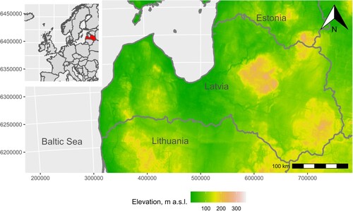
Latvia is located in the northwestern corner of the East European plain within the last Scandinavian ice sheet (Zelčs et al., 2011). The modern topography was mostly shaped by the multiple advances and retreats of the Scandinavian Ice sheet during the Pleistocene and modified by the more recent action of the Baltic Sea, fluvial and other terrestrial processes. The landscape can be described as a combination of plains corresponding to ice streams or ice flows and hilly uplands (Kalm, 2012). The present surface elevation ranges from a few metres below to 312 m above sea level (Figure 1).

Figure 1. Location and topography (GTOPO30, USGS, 1996) of the study area.

A topographic map of Latvia where the land surface elevation above sea level ranges between 0 and 300 m. In an inset map of Europe location of Latvia near the Baltic Sea is shown.

The Quaternary sediments are mostly glacial, glaciofluvial and glaciolimnic sediments (Dreimanis & Kārklin, 1997). The Quaternary cover is thinnest in lowland areas, often just a few metres but rarely absent, and thickest in upland regions, particularly in the central and eastern part of the country, reaching 200 m in the uplands (Zelčs et al., 2011).

At the bedrock surface, most Devonian sedimentary rocks are exposed except for the southwestern corner where more recent sedimentary rocks of Paleozoic and Mesozoic are present (Lukševičs et al., 2012). Generally, the sedimentary sequence has close to horizontal bedding with a few dislocations (Brangulis & Kaņevs, 2002). The Paleozoic and Mesozoic sedimentary strata are slightly inclined towards the south and southwest. As a result, in the northern part of the country, middle Devonian sandstones, siltstones, and clays, as well as dolomites, are exposed at the bedrock surface. In the central and southern regions, upper Devonian carbonate and mixed carbonate and terrigenous sedimentary formations and Mesozoic, mostly terrigenous sediments are exposed.

The largest (up to hundreds of kilometres) features of the bedrock surface topography largely reflect surface topography features – glacial uplands and lowlands (Gorlach et al., 2015). These features reflect denudation by major ice flows of numerous advances of the Scandinavian Ice Sheet during the Pleistocene. The same ice flows redeposited the material eroded upstream within the glacial uplands, masking the underlying bedrock from further glacial erosion (Kalm & Gorlach, 2014). On a kilometre scale, bedrock surface topography is determined by the bedrock composition. Cuesta-like escarpments or cliffs can be identified in places where hard Devonian dolomites are poorly consolidated terrigenous sediments.

There is widespread evidence of an existing network of paleo-incisions that are often referred to as buried valleys in the study region (Meirons et al., 1974; Rattas, 2007). These are deep and narrow valley-like incisions in the bedrock surface often filled with glacial, glaciofluvial and glaciolimnic deposits, sometimes distinguishable in the modern topography. According to the geological borehole database, the paleo-incision depths can exceed 300 m (average 70–80 m). The width of these features is from 10 to 20 m to a few kilometres, and they can be traced from a few hundred metres to up to 30 km. Initially, it was proposed that the buried valley systems are relict interglacial or pre-Quaternary river incisions (Skuodis, 1959). Later it was suggested that some of the incisions formed as tunnel valleys below the Scandinavian Ice Sheet by high-pressure subglacial streams (Vegt et al., 2012). In addition, it has been suggested that the pre-existing valley system was enhanced and modified by subglacial erosion (Vaher et al., 2010).

2.2. Borehole data

A geological borehole data set evaluated by Popovs et al. (2015), originally obtained from the Latvian Environment, Geology and Meteorology Centre and updated with the latest information (as of September 2020), was used. The dataset includes stratigraphic records from a borehole database covering the territory of Latvia (Takčidi, 1999). As supporting information, borehole data from similar databases for Estonia (Estonian Land board, 2015) and Lithuania (Belickas, 1999) were used. Lithuania and Estonian datasets were limited to a 50 km buffer zone along the Latvian border. Bedrock surface elevation from 17,481 wells in the Latvian mainland and 3071 wells from Lithuania and Estonia were used. No data from bordering areas of Belarus and Russia were available.

2.3. Data evaluation

Comprehensive quality control of the good dataset was carried out considering errors of recorded location and unrealistic stratigraphic sequences. The viability of borehole vertical reference was checked by a simple topological rule – the borehole cannot deviate more than the maximum possible vertical error against the Earth's surface for the national digital elevation model with a 20 m resolution (denoted maximal error in areas with poor ground surface visibility) (LĢIA, 2017 ). Such a large error margin accommodated decreased DEM accuracy along steep slopes of river valleys (Zhu et al., 2005). Unrealistic stratigraphic sequences are recorded in boreholes where either the order of stratigraphic units is mixed or where there are contradictions of entered thickness or depth values of stratigraphic units, resulting in a corrupted stratigraphic column and questionable legitimacy of the full borehole log. Such problems were screened algorithmically by checking the ascending sequence of the stratigraphic descriptors (Popovs et al., 2015). A total of 604 boreholes (2.94% from the initial dataset) were excluded from the dataset.

2.4. Buried paleo-incisions

Buried paleo-incisions pose a significant challenge for constructing a map of bedrock surface elevation. Knowledge about their distribution and morphology is limited and spatially uneven (Gorlach et al., 2015). Wells recovering buried incisions can be identified by comparing the Quaternary sequence with other nearby wells, but the incision morphology and extent remain unknown. Regardless of bedrock surface interpolation methods, since an insufficient number of wells within valley structures is available, hole-type effects will be observed around such wells. Therefore, the dataset was screened through cross-correlation and comparison of borehole descriptions of nearby wells, where 1223 wells (5.95% from the initial dataset) identified as recovering buried incisions were excluded from the interpolation of bedrock surface topography.

2.5. Surface construction

A multi-step euclidean distance tessellation method was used to construct a sub-Quaternary surface, forcing the bedrock surface to be equal to or less than the modern land surface elevation (LĢIA, 2017). This methodology assumes that the bedrock and land surface topography is uncorrelated except at the locations where Quaternary sediments are absent.

Standard geostatistical methods or simple linear interpolation were not suitable for the construction of a digital elevation model of the bedrock surface due to the spatial clustering of boreholes and the heterogeneity of the pre-Quaternary surface itself.

The tessellation was based on standard Thiessen polygons (Thiessen, 1911), widely used in many fields of modelling (Bodin et al., 2012; Ju et al., 2011). For each point, a polygon is constructed with a numeric value of the input where the input point serves as the centroid (the arithmetic centre of mass) (Figure 2(A)). In such a way, each of the two nearest polygons shares one edge section. However, we expand it further by calculating the mean value between each two nearest polygons and generating the point with this value in the middle of the coinciding boundary edge. This point set, together with the original point set, serves as input for each consecutive tessellation (Figure 2(C and D)). This approach bypasses the geometric effects of linear interpolation when applied to irregularly scattered data, gives a visually realistic surface, and produces a good fit against input data. Five-step tessellation was performed where the average area of the resulting polygon approximately coincides with the chosen resolution of the target surface (Figure 3).

Figure 2. Example of the multiple-step tessellation interpolation: An initial structure of input data and Thiessen polygons, (B and C) second and third tessellation. (a) Input borehole locations, (b) boundaries of initial Thiessen polygons, (c and e) centre points of boundaries of Thiessen polygons of previous tessellation, (d and e) boundaries of the second and third Thiessen polygons.

In three image frames (A, B and C), a stepwise increase in tessellation grid resolution is shown starting from original polygons defined around observations points.

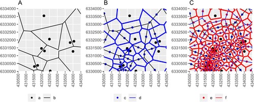
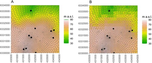
Figure 3. Example of transfer from tessellated height values to the regular grid. Black dots, location of boreholes. (A) Result of 5 step tessellation and (B) projection to the 250 m regular grid.

In two image frames, the differences between the interpolated elevation of tessellation polygons and their projection to a raster map are hardly noticeable.

2.6. Target grid resolution

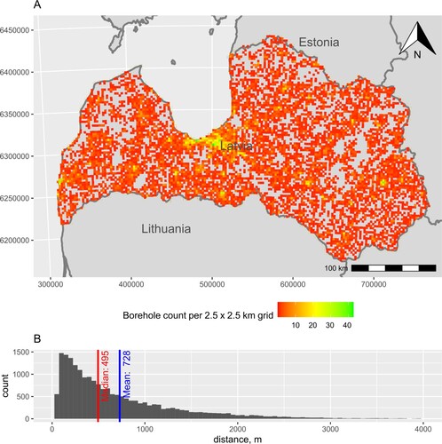
The chosen nominal grid cell size of the target model was 250 m. The target grid resolution was determined following the approach described by Hengl (2006). Accordingly, the sampling density of the input dataset corresponds to 205 m, while the finest legible grid resolution (a finest meaningful resolution that represents the most (95%) of surface and spatial objects) was 246 m. The density of available data varies radically, with the highest density along densely populated areas (Figure 4(A)). The median value between the nearest neighbouring wells is 492 m. In certain areas, the resolution could be increased; however, in large areas with sparse borehole coverage, the map resolution should be coarser than this. Therefore, the chosen nominal resolution corresponds to the rounded finest legible grid resolution proposed by Hengl (2006) for the regions with the largest density of boreholes. We maintain the overall finer resolution to preserve the spatial information where it is available.

Figure 4. Density of observation points (geological wells): (A) well distribution density on a 2.5 by 2.5 km grid and (B) histogram of the distance to the nearest neighbour borehole.

In image frame A, it is shown that the territory of Latvia is somewhat evenly covered by geological wells, with about 1 well on 2.5 km2. In frame B it can be observed that the distance between two nearest geological wells is up to 5 km, but it is heavily skewed towards smaller values; the median is 495 m and the mean is 728 m.

3. Results

The presented map (Main map, Figure 5) and bedrock surface digital elevation model provide a new digital dataset for future geological investigation and wide application in geological and hydrogeological modelling. Implementing the dataset in models will help advance geological research and integrate geological and ecological fields, providing the knowledge base for investigating groundwater-dependent ecosystems and interconnected networks of water flows at the surface and subsurface.

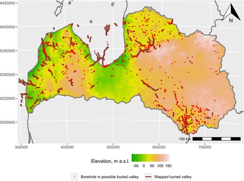
Figure 5. The Bedrock surface elevation of Latvia.

On the background of the bedrock surface elevation map of Latvia, known locations of paleo-incisions are shown.

3.1. Uncertainty assessment

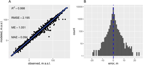
The uncertainty of the map was assessed in locations where more than one observation well was present within one 250 m grid cell. On average, the observed difference in bedrock surface elevation within a single grid cell mean error was 1.1 m (Figure 6). This is the average uncertainty of this map at grid cells with observation points. The average difference between interpolated and actual (unknown) bedrock surface elevation in grid cells with no observation points is likely to be higher.

Figure 6. Uncertainty assessment of the bedrock surface topography map: (A) cross-plot of observed and interpolated bedrock surface elevation and (B) error distribution of interpolated bedrock surface elevation (note the logarithmic vertical scale).

In the frame A of the image a good linear agreement between observed and interpolated bedrock surface elevation is shown with R2 = 0.998, RMSE = 2.195, ME = 1.051 and MAE = 0.094. In frame B, it is shown that a tiny fraction of interpolated values deviate from observed values of more than 10 m.

3.2. Data

The presented map is prepared as a formatted printable map (Main map) and georeferenced dataset comprising four raster bands: elevation of the bedrock surface above sea level, locations of boreholes used for the construction of the elevation of the bedrock surface, locations, where buried valleys in geological boreholes were uncovered, and thickness of Quaternary sediments.

4. Discussion

We have developed a new digital bedrock surface topography map of Latvia. In this discussion, we draw the attention of the reader to potential applications of the map and highlight some of the known issues. We use the case study of Kazu Leja (Kalvāns et al., 2021) to illustrate the important points raised during the discussion. This feature is a 3.6 km long, 0.3–0.8 km wide, and 40–45 m deep valley-like depression. Kazu Leja is a paleo valley incised into Devonian rocks and sediments and partly filled with late-glacial deposits (Juškevičs, 2000; Krievāns, 2015). It comprises a few interesting bedrock surface topography features: a cuesta-like escarpment of Devonian dolomites, partly buried paleo-incision and nearby river valleys as well as springs emerging from a karst aquifer. A 3D geological model of the Kazu Leja is available at the web page https://www.gprm.lu.lv/kazugrava-3d/

4.1. The modern river valleys

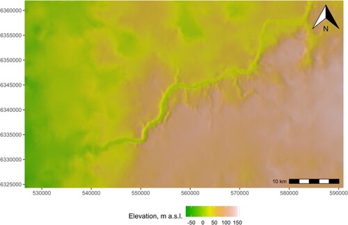
Many modern river valleys are incised in the bedrock surface, and in most cases they are well represented in our bedrock surface model (Figure 7). However, the methodology of representing these valleys in the bedrock surface elevation model has inherent flaws – these were cut into the interpolated surface of the bedrock by the intersection with the land surface model. Therefore, this approach disregards any alluvial sediments present in the river valley. Partly, the significance of the problem was curtailed by the relatively coarse resolution of the model – most of the river valleys were barely represented at 250 m resolution. Nevertheless, it remains an issue for the largest rivers like Gauja and Venta.

Figure 7. Representation of modern river Gauja valley in the bedrock surface model.

A detailed bedrock elevation map, 35 by 60 km section representation of a modern river valley is shown, where and bedrock surface elevation ranges from –50 to 150 m a.s.l.

4.2. The cuesta-like features and steep escarpments

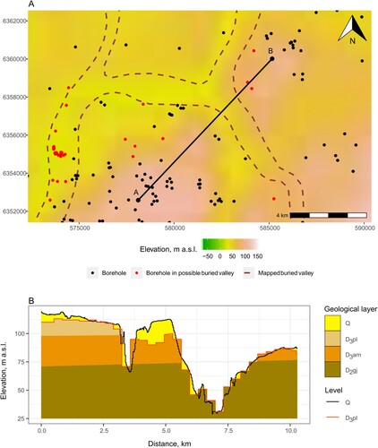
The cuesta-like features and steep escarpments are among the geological features best represented in the presented bedrock surface map as long as these are expressed at the land surface. The nature of their formation – the erosion of soft basement rock forming a pair of a steep slope and a gently inclined plateau – renders them suitable for representation on the map. At the first stage of map production, the smooth bedrock surface was interpolated between existing observation points. This was followed by the second stage, where the surface was forced to be at or below the land surface model (DEM), forming the escarpment front. The case study site, Kazu Leja, is located at the distribution margin of the dolomites of the Upper Devonian Pļaviņas formation (D₃pl), whih forms an escarpment or cuesta-like feature projected in the modern topography (Figure 8).

Figure 8. Bedrock topography (A) exposes paleo-incisions and cuesta-like features in the bedrock topography map and cross-section of the Kazu Leja case study (B). Due to different resolutions of land surface and bedrock surface elevation models, there are locations where nominal elevation bedrock grid cell elevation is above the actual land surface elevation.

The image shows a detailed representation of branching incised valleys in the bedrock surface elevation map. In a geological cross-section, it is demonstrated that the coarse resolution of bedrock surface elevation map compared to much finer resolution of land surface elevation model can lead to contradictions – apparent bedrock surface position above land surface – that need to be accounted for when conducting a detailed analysis.

4.3. Buried valleys (paleo-incisions)

Detailed mapping of paleo-incisions remains a major problem. On the main map, we show the paleo-incisions mapped before at a scale of 1:200,000 (Brangulis et al., 2000; Juskevics et al., 1997, 1998, 1999, 2003; Misans et al., 2001, 2002; Murnieks et al., 2002, 2004) as well as locations where these incisions are recovered in boreholes (Main map). However, examination of borehole log data shows numerous locations where the geological record suggests paleo-incisions, but their configuration is difficult to interpret at the presented mapping scale. We did not attempt to re-interpret previously mapped buried incisions as the resolution of available data was insufficient.

In the case of Kazu Leja (Figure 8), a buried incision was uncovered in a borehole at –30 m a.s.l. filled with till and sand and gravel deposits (Bendrupe & Arharova, 1981). The trajectory of the incision is marked by modern topography and proved by geological outcrops. However, apart from a single borehole, there were no data on its depth profile. A mixed fluvial and subglacial origin of the paleo-incision was proposed (Vaher et al., 2010). A fluvial valley is expected to have a smooth longitudinal profile, making possible interpolation between observation points. However, if the dominant form of their formation was pressurized subglacial tunnel valleys (Vegt et al., 2012), then their longitudinal profile is likely to be variable, complicated with sills and troughs; thus, extrapolation of a single observation along an imagined channel axis is likely to be speculative. Thus, the issue of paleo-incisions remains unresolved.

4.4. Applications

In the study region, the bedrock surface is the major discordance in the geological record, representing a sedimentary hiatus of up to about 380 million years – from Middle Devonian to Quaternary. Any geological model needs to account for the striking differences in sedimentary environment and processes during the Paleozoic and Quaternary, delineated by this sedimentary hiatus. Thus, the presented map will be a useful input for future work in geological modelling in the region.

4.4.1. Maps and models

The bedrock surface elevation map can be useful in geological construction models and deriving new high-resolution bedrock geology maps from these models. Pre- Quaternary strata formed in mostly shallow epicontinental seas (Lukševičs et al., 2012), with the sub-horizontal arrangement of the geological strata disrupted by a relatively small number of faults and low-amplitude folds (Brangulis & Kaņevs, 2002). These properties of regional bedrock geology were exploited by Virbulis et al. (2013) and Popovs et al. (2015) to create regional geological and hydrogeological models using interpolating marking layers among geological boreholes. Combining the presented map of bedrock surface topography and the geological modelling approach of Popovs et al. (2015) opens opportunities to produce high-resolution bedrock surface geological maps by intersecting the two data products. Furthermore, a bedrock surface lithology map can be produced by integrating the lithological descriptions from well databases into geological models and intersecting the result with bedrock surface topography. Such a map is currently is unavailable for the study region but would have many applications, for example, for geological prospecting and hydrogeological and ecological studies. Such a map would mimic the currently available Quaternary geology maps that integrate stratigraphical and lithological features.

4.4.2. Digital elevation analysis

The analysis of digital elevation maps is an established field in Earth sciences; however, it is primarily restricted to land surface topography. However, such features as coastline escarpments into bedrock, cuesta-like features along the margins of bedrock, carbonate formations, and elevated bedrock foundations underlying some of the uplands are exhibited in the bedrock topography map (see cross-sections in the main map). The resolution of the presented map does not match that of current land surface models, but it enables the rudimentary analysis of the bedrock surface elevation for geomorphology research.

4.4.3. Hydrogeology

Hydrogeological research can benefit from the availability of the presented bedrock elevation map. The groundwater flow is constrained by the underlying geology setting. For example, karst systems developed in carbonate aquifers can quickly funnel surface contaminants to the streams (Bakalowicz, 2005; Stevanović, 2018). To manage these hydrological systems properly, ensuring good groundwater and surface water status, detailed knowledge of the overburden and outcropping areas of these aquifers need to be known. Furthermore, the data must be presented in a consistent digital format, enabling seamless integration into modelling systems. It has been shown that detailed mapping of groundwater denitrification potential in cultivated lands can be a cost-effective measure in designating relevant, site-specific fertilizer application restrictions (Jacobsen & Hansen, 2016). Location of the interface between Quaternary and bedrock sediments can be an important parameter for assessing denitrification potential due to their contrasting hydrological properties or guiding the estimation of the depth of the redox interface (Hansen et al., 2014), i.e. the depth where anaerobic conditions facilitate denitrification.

Bedrock aquifer intersection by the land surface in the study region often supports groundwater-dependent ecosystems (Kalvāns et al., 2021; Koit et al., 2021) that are resilient due to consistent water supply but which might be vulnerable if groundwater suffers overexploitation or pollution. The presented map can be a valuable tool for predicting the locations of groundwater-dependent ecosystems and elaborating the conceptual hydrogeological models for such sites. Thus, the bedrock elevation map can be a useful input for water resources research.

4.4.4. Comparison of historic and new maps

A comparison was made between the newly generated map with newest historical map in scale 1:200,000 (Brangulis et al., 2000; Juskevics et al., 1997, 1998, 1999, 2003; Misans et al., 2001, 2002; Murnieks et al., 2002, 2004). The elevation isolines of the historical paper bedrock surface elevation map were digitized and a DEM created by the spline interpolation method. The historical DEM then was compared to geological well data available at the time when the historical map was finalized, i.e. before 2000 and well data established after 2000 and thus not used to create this historical map, and to the new map presented in this article (Figure 9).

Figure 9. Assessment of uncertainty between the historical bedrock map and new map: comparison of DEM created from published historic map isoline data with borehole data available at the time of map creation (A), with boreholes established later (B), and with a new map (C).

Image shows the comparison of old map compliance to borehole data available at the time of map creation in frame A, newer borehole data in frame B and cell to cell comparison to newly created map in frame C. Comparison of the old map against all borehole data highlights similar characteristics with underestimation up to about 100 m a.s.l. and similar values of statistical parameters, only with slightly smaller scattering for the comparison against newer data. A comparison of the old map and the newly created one shows insignificantly better values of statistical parameters, but characteristics are somewhat similar to comparison against boreholes.

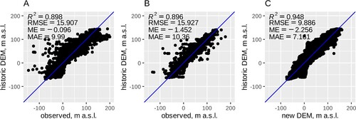
The comparison demonstrates that in all three cases, the error statistics are rather similar (Figure 9). The historical map is relatively robust, capturing all larger-scale features of the bedrock surface and accuracy of the map at the locations of new observations, which although relatively poor, have approximately the same accuracy as the accuracy at locations of observations available when the map was created. The error statistic between the new map and the old map is comparable to the old map and geological wells. The algorithm used for the creation of the new map that ensures almost a one-to-one match between the observation point and mapped elevation.

Overall, the new map is superior to the historical one as it better uses borehole data and better represents more local scale features allowing the new DEM model to be used not only at the regional scale but also in more local studies. While both maps give a similar insight to general characteristics of the bedrock surface, a large deviation of the historic map from borehole data for more than ±100 m limits the practical use of this map.

5. Conclusions

A bedrock surface elevation map for Latvia was elaborated using a geological borehole database complemented by known locations of buried paleo-incisions. The map is a useful data source for geology and hydrogeology-related research. The map is based on a bedrock surface digital elevation model that can be used as an input to modelling exercises to solve problems related to the exploration and management of geological resources and ecosystems.

Software

The Main Map was produced using ArcGIS Pro software from ESRI. To prepare the regional cross-sections, QGIS has been used. Final editing and PDF creation were carried out with Adobe Illustrator. Various map images of the manuscript were made using R-project (R Core Team, 2020).

Disclosure statement

No potential conflict of interest was reported by the author(s).

Data availability statement

A developed digital relief model of the Bedrock surface of Latvia used as a basis for the Bedrock surface map is available within the article’s supplementary materials. Restrictions apply to the availability of the primary data which were used under the license for this study. The primary data are property of relevant state authorities and can be requested from the Latvian Environmental, Geology and Meteorology Centre (www.meteo.lv), Geological Survey of Estonia (www.egt.ee) and Geological Survey of Lithuania (www.lgt.lt).

Additional information

Funding

This work was supported by the Latvian Council of Science [grant number lzp-2019/1-0165], Ministry of Education and Science Republic of Latvia [project no. ZD2010/AZ03 / AAP2016/B041] and ERDF [project No. 1.1.1.2/VIAA/3/19/524].

References

- Aleksans, O. (1991). Rezul’taty kompleksnoy gidrogeologicheskoy i inzhenerno-geologicheskoy s"yemki so s"yemkoy chetvertichnykh otlozheniy masshtaba 1:50000 dlya tseley melioratsii v predelakh listov 0-35-127-A,B,V,G;0-35-128-A,B,V,G i 0-35-129-A,V (Rezekne) (in Russian) Latv.
- Aleksans, O., & Ginters, G. (1988). Otchet o rezul’tatakh kompleksnoy gidrogeologicheskoy i inzhenerno-geologicheskoy s’yemki so s’yemkoy chetvertichnykh otlozheniy masshtaba 1:50000 dlya tseley meliorativnogo stroitel’stva v predelakh listov 0-35-90-A,B,V,G; 0-35-91-A,B,V,G i 0-35-92-A,V.
- Bakalowicz, M. (2005). Karst groundwater: A challenge for new resources. Hydrogeology Journal, 13(1), 148–160. https://doi.org/10.1007/s10040-004-0402-9
- Belickas, J. (1999). GEOLIS - geological information system. Science and Arts of Lithuania, 23, 554–556.
- Bendrupe, L., & Arharova, T. (1981). Geologicheskaya karta (dochetvertichnyye otlozheniya) mashtaba 1:50 000. V: Prilozheniye k otchet o gruppovoy geologicheskoy syemke masshtaba 1:50 000 Gauyskogo natsionalnogo parka (Latvian geologicla archive No 9855).
- Bodin, T., Salmon, M., Kennett, B. L. N., & Sambridge, M. (2012). Probabilistic surface reconstruction from multiple data sets: An example for the Australian Moho. Journal of Geophysical Research: Solid Earth, 117(10), 1–13. https://doi.org/10.1029/2012JB009547
- Brangulis, A., Juskevics, V., Kondratjeva, S., Gavena, I., & Pomeranceva, R. (2000). Latvijas geologiska karte, merogs 1:200000, 43.lapa - Riga, 53.lapa - Ainazi (paskaidrojuma teksts un kartes) (in Latvian) Latvian State Geological Fund No. 12301.
- Brangulis, A. J., & Kaņevs, S. (2002). Latvian tectonics (in Latvian with English summary) (Misāns, Jā). Valsts ģeoloģijas dienests.
- Chen, Z., Auler, A. S., Bakalowicz, M., Drew, D., Griger, F., Hartmann, J., Jiang, G., Moosdorf, N., Richts, A., Stevanovic, Z., Veni, G., & Goldscheider, N. (2017). The World Karst Aquifer Mapping project: Concept, mapping procedure and map of Europe. Hydrogeology Journal, 25(3), 771–785. https://doi.org/10.1007/s10040-016-1519-3
- Dreimanis, A., & Kārklin, O. L. (1997). Latvia. In E. Moores & R. Fairbridge (Eds.), Encyclopedia of European and Asian regional geology (pp. 498–504). Kluwer Academic Publishers. https://doi.org/10.1007/1-4020-4495-X_59
- Drikis, V. (1980). Otchet o rezul’tatakh kompleksnoy gidrogeologicheskoy i inzhenerno-geologicheskoy s’yemki so s’yemkoy chetvertichnykh otlozheniy masshtaba 1:50000 dlya tseley meliorativnogo stroitel’stva v Bausskom rayone (1977-1980 g.g.). V 4-kh tomakh (in Russian) Latv.
- Estonian Land board. (2015). Borehole database. https://geoportaal.maaamet.ee/docs/geoloogia/andmed/puuraugud.zip?t=20180404142058
- Freimanis, A., Meirons, Z., & Hvedcena, O. (1966). Otchet o rezul’tatakh geologo-gidrogeologicheskoy s’yemke m-ba 1:200000 na territorii lista 0-34-XXX (Kurzemskaya GSP) 1965-1966 g.g. (in Russian) Latvian State Geological Fund No. 06447.
- Gavrilova, A., Birgere, L., Straume, J., & Bychko, G. (1966). Otchet o rezul’tatakh kompleksnoy geologo-gidrogeologicheskoy s’yemki m-ba 1:200000 na territorii lista 0-34-XXXV Yuzhno-Latviyskaya GSP (g.Riga) 1964-1966 g.g. (in Russian) Latvian State Geological Fund No. 06473.
- Gavrilova, A., Birgere, L., Straume, J., Bychko, G., Emulis, E., Kipena, M., & Ljarskaja, L. (1967). Otchet o rezul’tatakh kompleksnoy geologo-gidrogeologicheskoy s’yemki masshtaba 1:200000 na territorii lista 0-34-XXXVI (Yuzhno-Latv.GSP) 1965-67 g.g. (in Russian) Latvian State Geological Fund No. 07152.
- Gavrilova, A., Feldmane, L., Straume, J., Birgere, L., & Bychko, G. (1962). Otchet Ogrskoy GSP po rabotam 1959-60 g.g. (geologicheskoye stroyeniye i gidrogeologicheskiye usloviya territorii lista 0-35-XXV) (in Russian) Latvian State Geological Fund No. 03104.
- Gavrilova, A., & Ginters, G. (1975). Otchet o gruppovoy opytno-proizvodstvennoy kompleksnoy geologo-gidrogeologicheskoy s’yemke m-ba 1:50000 ter-ii listov 0-34-129-A,B,V,G, 0-34-130-A,B,G (severnaya polovina) (in Russian) Latvian State Geological Fund No. 09429.
- Gavrilova, A., & Ginters, G. (1978). Otchet o gruppovoy geologicheskoy s’yemke m-ba 1:50000 (g.Yekabpils) 1976-1978 g. (in Russian) Latvian State Geological Fund No. 09596.
- Gavrilova, A., & Straume, J. (1963). Otchet o rezul’tatakh kompleksnoy geologo-gidrogeologicheskoy s’yemki masshtaba 1:200000 na territorii lista 0-34-XXXIV (Primorskaya geologos’yemochnaya partiya) 1961-1963 g.g. (in Russian) Latvian State Geological Fund No. 03667.
- Ginters, G., Aleksans, O., & Vilcans, J. (1986). Otchet o kompleksnoy gidrogeologicheskoy i inzhenerno-geologicheskoy s’yemke so s’yemkoy chetvertichnykh otlozheniy masshtaba 1:50000 dlya tseley meliorativnogo stroitel’stva v predelakh listov 0-35-102-A,B,V,G (Gulbene) 1983-1986 g.g. (in Russian) Latvia.
- Ginters, G., Aleksans, O., Vilcans, J., & Meirons, Z. (1985). Otchet o kompleksnoy gidrogeologicheskoy i inzhenerno-geologicheskoy s"yemke so s"yemkoy chetvertichnykh otlozheniy masshtaba 1:50000 dlya tseley meliorativnogo stroitel’stva v predelakh listov 0-35-101 A,B,V,G (Jaunpiebalga) 1982-1985 g.g. (in Russian) L.
- Gorlach, A., Kalm, V., & Hang, T. (2015). Thickness distribution of quaternary deposits in the formerly glaciated part of the East European plain. Journal of Maps, 11(4), 625–635. https://doi.org/10.1080/17445647.2014.954646
- Hansen, A. L., Christensen, B. S. B., Ernstsen, V., He, X., & Refsgaard, J. C. (2014). A concept for estimating depth of the redox interface for catchment-scale nitrate modelling in a till area in Denmark. Hydrogeology Journal, 22(7), 1639–1655. https://doi.org/10.1007/s10040-014-1152-y
- Hengl, T. (2006). Finding the right pixel size. Computers and Geosciences, 32(9), 1283–1298. https://doi.org/10.1016/j.cageo.2005.11.008
- Jacobsen, B. H., & Hansen, A. L. (2016). Economic gains from targeted measures related to non-point pollution in agriculture based on detailed nitrate reduction maps. Science of the Total Environment, 556, 264–275. https://doi.org/10.1016/j.scitotenv.2016.01.103
- Jankins, J., Hvedcena, O., & Meirons, Z. (1969). Otchet o rezul’tatakh kompleksnoy geologo-gidrogeologicheskoy s’yemki m-ba 1:200000 na territorii lista 0-34-XXIX-1966-1969 g. (in Russian) Latvian State Geological Fund No. 08556.
- Jankins, J., Meirons, Z., Murnieks, A., & Arharova, T. (1973). Otchet o rezul’tatakh geologo-gidrogeologicheskoy s’yemki masshtaba 1:200000 na territorii lista 0-35-XXXIV (Rezekne) 1968-1973 g.g (in Russian) Latvian State Geological Fund No. 09227.
- Jankins, J., Murnieks, A., & Murniece, S. (1975). Otchet o doizuchenii territorii lista 0-35-XXVIII (Balvi) s tsel’yu podgotovki k izdaniyu geologicheskikh kart m-ba 1:200000 (in Russian) Latvian State Geological Fund No. 09388.
- Jansons, A., Bendrupe, L., & Turkina, L. (1965). Otchet o rezul’tatakh kompleksnoy geologo-gidrogeologicheskoy s’yemki m-ba 1:50000 na territorii listov 0-35-97-V i 0-35-109-A (Daugavskaya GSP) 1963-65 g.g. (in Russian) Latvian State Geological Fund No. 05767.
- Jansons, A., Bendrupe, L., Turkina, L., & Straume, J. (1967). Otchet o rezul’tatakh geologo-gidrogeologicheskoy s’yemki masshtaba 1:50000 listov 0-35-97-G i 0-35-109-B (in Russian) Latvian State Geological Fund No. 07340.
- Jansons, A., Bendrupe, L., Turkina, L., & Straume, J. (1971). Otchet o rezul’tatakh gidrogeologicheskoy s’yemki m-ba 1:50000 listov 0-34-107-G, 0-34-119-B, 0-34-120-A,B dlya vodosnabzheniya gor.Jurmala 1967-1971 gody (in Russian) Latvian State Geological Fund No. 09050.
- Ju, L., Ringler, T., & Gunzburger, M. (2011). Voronoi tessellations and their application to climate and global modeling. In P. Lauritzen, C. Jablonowski, M. Taylor, & R. Nair (Eds.), Numerical techniques for global atmospheric models. Lecture notes in computational Science and engineering (Vol. 80, pp. 313–342). Springer. https://doi.org/10.1007/978-3-642-11640-7_10
- Juškevičs, V. (2000). Kvartāra nogulumi. Latvijas ģeoloģiskā karte, M 1:200 000, 43-45. lapa - Rīga - Ainaži, Paskaidrojuma teksts. (O. Āboltiņš & V. Kuršs, Eds.). Valsts Ģeoloģijas Dienests.
- Juskevics, V., Kondratjeva, S., Murnieks, A., & Murniece, S. (1997). Latvijas geologiska karte, merogs 1:200000. 31.lapa - Liepaja (paskaidrojuma raksts) (in Latvian) Latvian State Geological Fund No. 11728.
- Juskevics, V., Kondratjeva, S., Murnieks, A., & Murniece, S. (1998). Latvijas geologiska karte. Merogs 1:200000. 41. lapa - Ventspils (paskaidrojuma teksts un kartes) (in Latvian) Latvian State Geological Fund No. 11871.
- Juskevics, V., Misans, J., Murnieks, A., & Skrebels, J. (2003). Latvijas geologiska karte, merogs 1:200000, 34.lapa-Jekabpils, 24.lapa-Daugavpils (paskaidrojuma teksts un kartes) (in Latvian) Latvian State Geological Fund No. 14045.
- Juskevics, V., Murnieks, A., & Misans, J. (1999). Latvijas geologiska karte, merogs 1:200000, 42.lapa - Jurmala (paskaidrojuma teksts un kartes) (in Latvian) Latvian State Geological Fund No. 12300.
- Juskevics, V., & Vihots, L. (1978). Otchet o kompleksnoy gidrogeologicheskoy i inzhenerno-geologicheskoy s’yemke m-ba 1:50000 v r-ne g.Daugavpils 1974-1978 g.g. (in Russian) Latvian State Geological Fund No. 09588.
- Kajak, K. (1976). Otchet Yuzhno-estonskogo otryada o kompleksnoy geologo-gidrogeologicheskoy s’yemke m-ba 1:200000 yuzhnoy chasti ter-ii 0-35-XXII (v okrestnostyakh Aluksne, Misso, Kachanovo) za 1974-1975 g. (in Russian) Latvian State Geological Fund No. 09433.
- Kalm, V. (2012). Ice-flow pattern and extent of the last Scandinavian Ice Sheet southeast of the Baltic Sea. Quaternary Science Reviews, 44, 51–59. https://doi.org/10.1016/j.quascirev.2010.01.019
- Kalm, V., & Gorlach, A. (2014). Impact of bedrock surface topography on spatial distribution of quaternary sediments and on the flow pattern of late Weichselian glaciers on the East European Craton (Russian Plain). Geomorphology, 207, 1–9. https://doi.org/10.1016/j.geomorph.2013.10.022
- Kalvāns, A., Popovs, K., Priede, A., Koit, O., Retiķe, I., Bikše, J., Dēliņa, A., & Babre, A. (2021). Nitrate vulnerability of karst aquifers and associated groundwater-dependent ecosystems in the Baltic region. Environmental Earth Sciences, 80(18), 628. https://doi.org/10.1007/s12665-021-09918-7
- Koit, O., Tarros, S., Joonas, P., Küttim, M., Abreldaal, P., Sisask, K., Vainu, M., Terasmaa, J., Retike, I., & Polikarpus, M. (2021). Contribution of local factors to the status of a groundwater dependent terrestrial ecosystem in the transboundary Gauja-Koiva River basin, North-Eastern Europe. Journal of Hydrology, 600, Article 126656. https://doi.org/10.1016/j.jhydrol.2021.126656
- Krievāns, M. (2015). Hidrogrāfiskā tīkla veidošanās lejas Gaujas senielejai pieguļošajā teritorijā vēlā Vislas apledojuma deglaciācijas laikā (Issue 28) [University of Latvia]. https://dspace.lu.lv/dspace/handle/7/28297
- LĢIA. (2017). Digitālais augstuma modelis (Digital elevation model). Retrieved June 17, 2021, from https://www.lgia.gov.lv/en/Digitālais%reljefa%modelis
- Lukševičs, E., Stinkulis, Ģ, Mūrnieks, A., & Popovs, K. (2012). Geological evolution of the Baltic Artesian Basin. In A. Dēliņa, A. Kalvāns, S. Tomas, U. Bethers, & V. Vircavs (Eds.), Highlights of groundwater research in the Baltic Artesian Basin (pp. 7–52). University of Latvia.
- Meirons, Z., Straume, J., & Juškevics, V. (1974). Kharakteristika podchetvertichnoi poverkhnosti Latvii i nekotorye voprosy formirovania pogrebyonnykh dolin (Characterisation of pre-Quaternary topography of Latvia and some problems of formation of buried valleys). In I. Danilans (Ed.), Voprosy Chetvertichnoi Geologii VII. (Problems of Quaternary Geology VII) (pp. 9–21). Riga: Zinātne (in Russian).
- Mironovs, G., Vacele, V., Vasiljeva, V., & Karpickij, V. J. (1962). Otchet Vidzemskoy kompleksnoy GSP po rabotam 1959-60 g.g. (geologicheskoye stroyeniye i gidrogeologicheskiye usloviya territorii lista 0-35-XXVI) (in Russian) Latvian State Geological Fund No. 03109.
- Misans, J., Meirons, Z., & Murnieks, A. (2002). Latvijas geologiska karte, merogs 1:200000, 33.lapa-Ogre (paskaidrojuma teksts un kartes) (in Latvian) Latvian State Geological Fund No. 14044.
- Misans, J., Murnieks, A., & Strautnieks, I. (2001). Latvijas geologiska karte, merogs 1:200000. 32.lapa-Jelgava (paskaidrojuma teksts un kartes) (in Latvian) Latvian State Geological Fund No. 12444.
- Murnieks, A., Juskevics, V., & Misans, J. (2002). Latvijas geologiska karte, merogs 1:200000 44.-45.-54.lapa Aluksne-Vilaka-Valka (paskaidrojuma teksts un karte) (in Latvian) Latvian State Geological Fund No. 13120.
- Murnieks, A., Meirons, Z., & Misans, J. (2004). Latvijas geologiska karte, merogs 1:200000. 25.lapa - Indra, 35.lapa - Rezekne. Paskaidrojuma teksts un kartes (in Latvian) Latvian State Geological Fund No. 14707.
- Murnieks, A., & Murniece, S. (1979). Otchet o kompleksnoy gidrogeologicheskoy i inzhenerno-geologicheskoy s’yemke masshtaba 1:50000 v rayone nas.p.Engure (in Russian) Latvian State Geological Fund No. 09625.
- Paulen, R. C., McClenaghan, M. B., Harris, J. R. (2006). Bedrock toropgraphy and drift thickness models from the Timmins area, Northeastern Ontario: An application of GIS to the Timmins overburden drillhole database. In J. Harris & D. Wright (Eds.), GIS for the Earth Sciences (vol. 44, pp. 413–434). St. John's: Geological Association of Cananda.
- Podgurskis, V., Meirons, Z., & Arharova, T. (1985). Otchet o gruppovoy geologicheskoy s’yemke masshtaba 1:50000 na territorii listov 0-34-91-G; 0-34-92-A,B,V,G; 0-34-103–B,G; 0-34-104-A,B,V,G (g.Ventspils) (in Russian) Latvian State Geological Fund No. 10279.
- Popovs, K., Saks, T., & Jātnieks, J. (2015). A comprehensive approach to the 3D geological modelling of sedimentary basins: Example of Latvia, the central part of the Baltic Basin. Estonian Journal of Earth Sciences, 64(2), 173–188. https://doi.org/10.3176/earth.2015.25
- Rattas, M. (2007). Spatial distribution and morphological aspects of eskers and bedrock valleys in north Estonia: Implications for the reconstruction of a subglacial drainage system under the Late Weichselian Baltic Ice stream. In P. Johansson & P. Sarala (Eds.), Geological Survey of Finland, Special Paper 46, Applied Quaternary research in the central part of glaciated terrain proceedings of the INQUA Peribaltic Group Field Symposium 2006 (pp. 63–68). Espoo: Geological Survey of Finland.
- R Core Team. (2020). R: A language and environment for statistical computing. R Foundation for Statistical Computing. https://www.r-project.org/
- Skuodis, V. (1959). O drevney pogrebennoy doline v rayone vpadeniya r. Lautse v r. Daugava (About the ancient buried valley in the area of the confluence of the river. Lauze in the r. Daugava; in Russian). In Geologiya doliny reki Daugava (Geology of the Daugava River Valley). Izdatel’stvo Akademiya nauk Latviyskoy SSR.
- Stevanović, Z. (2018). Global distribution and use of water from karst aquifers. Geological Society, London, Special Publications, 466(1), 217–236. https://doi.org/10.1144/SP466.17
- Takčidi, E. (1999). Datu bāzes “Urbumi” dokumentācija [Documentation of the database “Boreholes”].
- Thiessen, A. M. (1911). Precipitation average for large areas. Monthly Weather Review, 39(6), 1082–1084. https://doi.org/10.1175/1520-0493(1911)39<926:DNGB>2.0.CO;2
- Tracevskis, G. (1989). Otchet Zap.partii o gidrogeologicheskoy s’yemke s inzhenerno-geologicheskoy s’yemkoy i geologicheskoy s’yemkoy dochetvetvertichnykh i chetvertichnykh otlozheniy masshtaba 1:50000 (in Russian) Latvian State Geological Fund No. 10686.
- Tracevskis, G. (1993). Rezul’taty geologicheskoy s’yemki masshtaba 1:50000 territorii listov O-34-81-V,G; O-34-82-V; O-34-93-A,B,V,G; O-34-94-A,B,V,G; O-34-95-V; O-34-105-A,B; O-34-106-A,B (Talsi, Kolka) (in Russian) Latvian State Geological Fund No. 11035.
- Tracevskis, G., Anikejeva, R., Briviba, J., & Bychko, A. (1984). Otchet o gruppovoy s’yemke masshtaba 1:50000 na territorii listov 0-34-127-A,B,V,G i 0-34-139-A,B (g.Liepaja) (in Russian) Latvian State Geological Fund No. 10180.
- Tracevskis, G., Juskevics, V., & Bogdanovs, A. (1969). Otchet o kompleksnoy geologo-gidrogeologicheskoy i inzhenerno-geologicheskoy s’yemke m-ba 1:200000 na territorii listov 0-34-XXII, XXIII, XXIV. Severo-Latviyskaya GSP 1967-1969 g. (in Russian) Latvian State Geological Fund No. 08555.
- Tracevskis, G., Juskevics, V., & Polivko, J. (1965). Otchet o kompleksnoy geologo-gidrogeologicheskoy s’yemke masshtaba 1:200000 na territorii lista 0-35-XX (Severo-Latviyskaya GSP) (in Russian) Latvian State Geological Fund No. 05870.
- Tracevskis, G., Juskevics, V., Polivko, J., & Bicko, A. (1967). Otchet o kompleksnoy geologo-gidrogeologicheskoy i inzhenerno-geologicheskoy s’yemke masshtaba 1:200000 na territorii lista 0-35-XIX (in Russian) Latvian State Geological Fund No. 07142.
- Tracevskis, G., Juskevics, V., Polivko, J., & Bychko, A. (1964). Otchet o kompleksnoy geologo-gidrogeologicheskoy s’yemke masshtaba 1:200000 na territorii yuzhnoy poloviny lista 0-35-XXI (Severo-Latviyskaya GSP) (in Russian) Latvian State Geological Fund No. 04154.
- Ulgis, M. (1981). Otchet o kompleksnoy gidrogeologicheskoy i inzhenerno-geologicheskoy s’yemke so s’yemkoy chetvertichnykh otlozheniy masshtaba 1:50000 dlya tseley meliorativnogo stroitel’stva na Vidzemskoy vozvyshennosti (in Russian) Latvian State Geological Fund No 09811.
- Ulgis, M. (1983). Otchet o kompleksnoy gidrogeologicheskoy i inzhenerno-geologicheskoy s’yemke so s’yemkoy chetvertichnykh otlozheniy masshtaba 1:50000 (..) listov 0-35-139-A,B,V,G (Aglona) 1980-1983 g.g. (in Russian) Latvian State Geological Fund No. 10035.
- USGS. (1996). GTOPO30 Documentation. U.S. Geological Survey (USGS). https://lta.cr.usgs.gov/sites/default/files/GTOPO30_README.doc
- Vaher, R., Miidel, A., Raukas, A., & Tavast, E. (2010). Ancient buried valleys in the city of Tallinn and adjacent area rein. Estonian Journal of Earth Sciences, 59(1), 37–48. https://doi.org/10.3176/earth.2010.1.03
- Vegt, V. D., Janszen, A., & Moscariello, A. (2012). Tunnel valleys: Current knowledge and future perspectives. Geological Society, London, 368(1), 75–97. https://doi.org/10.1144/SP368.13
- Vetrennikovs, V., & Bendrupe, L. (1976). Otchet o rezul’tatakh kompleksnoy geologo-gidrogeologicheskoy i inzhenerno-geologicheskoy s’yemki m-ba 1:200000 na ter-ii lista 0-35-XXXI v predelakh LSSR 1974-1976 g. (in Russian) Latvian State Geological Fund No. 09469.
- Virbulis, J., Bethers, U., Saks, T., Sennikovs, J., & Timuhins, A. (2013). Hydrogeological model of the Baltic Artesian Basin. Hydrogeology Journal, 21(4), 845–862. https://doi.org/10.1007/s10040-013-0970-7
- Zelčs, V., Markots, A., Nartišs, M., & Saks, T. (2011). Pleistocene glaciations in Latvia. In J. Ehlers, P. L. Gibbard, & P. D. Hughes (Eds.), Quaternary glaciations - extent and chronology (pp. 221–229). Elsevier.
- Zhu, C., Shi, W., Li, Q., Wang, G., Cheung, T. C. K., Dai, E., & Shea, G. Y. K. (2005). Estimation of average DEM accuracy under linear interpolation considering random error at the nodes of TIN model. International Journal of Remote Sensing, 26(24), 5509–5523. https://doi.org/10.1080/10245330500169029