Oxia Planum, Mars, classified using the NOAH-H deep-learning terrain classification system

ABSTRACT

We present a map of Oxia Planum, Mars, the landing site for the ExoMars Rover. This shows surface texture and aeolian bedform distribution, classified using a deep learning (DL) system. A hierarchical classification scheme was developed, categorising the surface textures observed at the site. This was then used to train a DL network, the ‘Novelty or Anomaly Hunter – HiRISE’ (NOAH-H). The DL applied the classification scheme across a wider area than could have been mapped manually. The result showed strong agreement with human-mapped areas reserved for validation. The resulting product is presented in two ways, representing the two principle levels of the classification scheme. ‘Descriptive classes’ are purely textural in nature, making them compatible with a machine learning approach. These are then combined into ‘interpretive groups’, broader thematic classes, which provide an interpretation of the landscape. This step allows for a more intuitive analysis of the results by human users.

KEYWORDS:

• Machine learning
• Mars surface
• geomorphology
• ExoMars
• deep learning
• rover planning

Key Policy Highlights

• A Map of Oxia Planum has been created, showing variations in surface texture across the planned ExoMars Rosalind Franklin rover landing site.

• The landscape of Oxia Planum was classified using a suite of 14 descriptive classes.

• A deep learning convolutional neural network was trained to predict these classes in further HiRISE images, which had not been used for training.

• The resulting classified rasters were orthorectified and mosaicked using ArcGIS.

• The resulting map will be used as an input to rover traversability assessments for Rosalind Franklin and is already being used to unravel the aeolian history of Oxia Planum.

1. Introduction

Oxia Planum has been selected as the landing site for the European Space Agency’s ExoMars Rosalind Franklin Rover (Vago et al., 2017), where the rover intends to seek evidence of past and present life and characterise the geochemical environment in the near subsurface. As part of the ongoing process to characterise the ExoMars landing site, a Deep Learning (DL) terrain classification system, the ‘Novelty or Anomaly Hunter – HiRISE’ (NOAH-H), was trained to distinguish different surface textures and aeolian bedform morphologies. The system uses 25 cm/pixel images from the High-Resolution Imaging Science Experiment (HiRISE) camera aboard NASA’s Mars Reconnaissance Orbiter spacecraft (McEwen et al., 2007). These are the highest resolution satellite images presently available for Mars. There is nearly full coverage of the proposed ExoMars landing site (Figure 1). The selected HiRISE images cover an area of ∼3000 km², equivalent to ∼50 billion HiRISE pixels. It is thus extremely time-consuming to reliably survey such a data volume manually using the full HiRISE resolution data, even for the large team associated with the ExoMars rover mission.

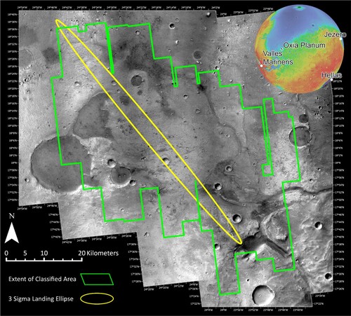
Figure 1. Context map showing the location of the classified area (green) within Oxia Planum, and its position relative to a 3-sigma landing uncertainty ellipse (yellow) modelled for a launch at the start of the 2022 launch window. Landing ellipses for future launch opportunities in preparation are planned to target the same location. CTX mosaic by Fawdon et al. (2021, https://doi.org/10.21954/ou.rd.16451220.v1). Inset: Mars Orbiter Laser Altimeter (MOLA) elevation globe showing relative location of prominent geographic features and the landing sites of other rover missions.

The extent of the classified area is shown to mostly contain an example 3-sigma landing ellipse. A globe of Mars shows the location of the site, on the planetary dichotomy between Arabia Terra and Chryse Planitia.

Topographic information from digital elevation models was not included in the training dataset, so the classification is based solely on 2D, textural information recovered from the red band HiRISE images themselves. Limiting our classification to areas with topographic data would have restricted where the tool could be used and would have required a more complex algorithm for little gain. In the case of aeolian bedforms and upstanding ‘rugged’ terrains 3D context can be inferred from the 2D HiRISE image. While topographic data will be required for a full traversability analysis, this is better accomplished by comparing the classification with a digital elevation model after the fact, rather than trying to incorporate the topographic information into the DL model and so locking that component of traversability assessment into a ‘black box’ where its impact would be harder to disentangle from the impact of surface texture.

Not only is extracting qualitative information from observations of remote sensing images time intensive, it is also challenging to perform as relatively few experts are available globally to complete such work, and their time is often oversubscribed. Much of the process of compiling a geomorphological map is interpretive in nature, requiring an understanding of how landscapes evolve and develop over geological timescales. Even determining how to classify variations in surface textures into useable groups requires experience and expertise, especially as classes sometimes form a continuum. Interpretations are made using contextual information as well as the morphology of a specific landform, and the discussions and observations that arise from this process are vital for building an understanding of the site. However, the most time-consuming part of the process is the interrogation of the imaging data and the recording of the spatial location and extent of different textures or features prior to interpreting any patterns.

This first stage of map-making is largely descriptive and can thus be framed as an image segmentation task, utilising surface texture, but without the situational evidence that will be required to later interpret the results. This makes it possible to train a DL system to recognise and segment basic terrain classes. These do not comprise strict geological units. Rather they are fundamental textures, described in terms of surface roughness and the arrangement of distributed features. These textures are expected to vary from one unit to another. Assemblages of these textures, in different combinations, could provide characteristic indicators of geological or geomorphological units, paleo-surfaces, or highlight textural transitions, which could later be interpreted as unit boundaries. These textures can comprise both bedrock and surficial materials (i.e. bedforms). NOAH-H is thus intended to perform ‘triage’ on unmanageably large datasets and provide a human mapper with a richer product that can inform their more in-depth study of the site.

The aim of the study was to classify all relevant HiRISE images of the landing site using the NOAH-H system. These images were precisely georeferenced and mosaicked so that the final map would form a solid foundation for future traversability assessment of the site.

2. Study area

Oxia Planum is a low relief region on the western margin of Arabia Terra on the edge of Chryse Planitia (Fawdon et al., 2021). It contains abundant exposures of phyllosilicate-bearing bedrock and a fan-shaped sedimentary structure at the terminus of an ancient fluvial channel system (Fawdon et al., 2021; Quantin-Nataf et al., 2021). The Oxia Planum region hosts numerous erosional remnants, such as rounded buttes (McNeil et al., 2021), inverted channels (Fawdon, Balme, et al., 2022), and periodic bedrock ridges (Favaro et al., 2021), all indicative of low-intensity erosion processes operating for a long period of time. The site at Oxia Planum was chosen because of this widespread bedrock exposure which may contain physical and chemical biomarkers (Summons et al., 2011), as well as compatibility with the EDL (entry descent and landing) requirement of the lander platform and the mobility capabilities of the ExoMars Rosalind Franklin rover.

3. Materials and methods

The development of the NOAH-H system is described in depth in Barrett et al. (2022). The landscapes of Oxia Planum (Fawdon et al., 2021; Quantin-Nataf et al., 2021) and nearby Mawrth Vallis (Poulet et al., 2020) were surveyed using HiRISE images, in total, 14 terrain types were identified, covering the full variety of surfaces and bedforms present at both sites. The classification scheme was themed around the traversability of the surface, with the intention that these ontological classes could provide one component of in-depth traversability assessment when combined with in situ data and engineering constraints of the rover. It should be noted, however, that rover-specific parameters were not included in the model directly, so the classified maps only represent the textural characteristics of the surface as seen in HiRISE images. An example of a classified area is shown in (Figure 2).

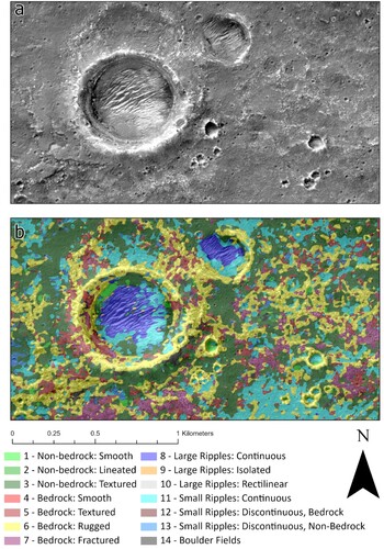
Figure 2. Comparison of (a) HiRISE image and (b) NOAH-H classified raster showing a small crater at 17.81°N, 23.91°W. The crater rim and the edge of the ejecta blanket are picked out as rugged bedrock (yellow). Fields of large ripples are found in the interiors of both craters (dark blue) while small ripples occur throughout (cyan). The area outside of the craters is primarily a mixture of textured non-bedrock (green) and exposures of textured (red) or fractured (purple) bedrock. (HIRISE Image 019084_1985_RED, Credit: NASA/JPL/UofA.)

Two craters, one larger and one smaller are filled with aeolian bedforms of various sizes, consistently oriented north-east to south-west. One inset shows a black and white HiRISE image, while the other is coloured to indicate how the landscape has been classified. The classification is mostly accurate, picking out the crater rims, the bedforms, and many more subtle variations.

The DL system frames the task of classifying the landscape as a semantic segmentation problem, where the model learns to recognise characteristics of the landscape from training information. Geological or geomorphological remote sensing mapping requires both description and interpretation. The former can be approached using semantic segmentation while the later, presently, cannot. This means that the classification must be based purely on textural parameters, rather than on the situational or contextual information ordinarily available to a human mapper. However, while this interpretive dimension is unknown to the model itself, it is vital for human geologists to consider the meaning of the results. It should be noted that human classification is also highly subjective.

Therefore, a hierarchical approach was taken. The network classifies the terrain into 14 ‘descriptive classes’. These were then combined into broader thematic groups (Table 1, Figure 4) to produce an interpretive layer of the model. These are termed ‘interpretive groups’. Characteristics of the landscape were interpreted based on the assemblages of descriptive classes observed. The list of classes is shown in Table 1, which also indicates how they were grouped and an estimate of their likely traversability. Type examples of these textures are shown in the map key to Figures 3 and 4, which also show the grouping strategy.

Figure 3. Map sheet: descriptive classes. GIS-ready files are available as supporting material and we encourage readers to download these in order to view the product at full resolution and symbolise it as needed to better highlight the more subtle variations.

A coloured map shows descriptive classes across the whole study area. Bedrock is most prominent in the centre of the image, while more non-bedrock predominates to the north-east. Concentrations of aeolian cover are confined to craters, and in South Neocoogoon Vallis in the south-east of the map. The map key shows a swatch of each colour, alongside a type example of the class.

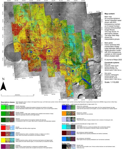
Figure 4. Map sheet: interpretive groups. GIS-ready files are available as supporting material and we encourage readers to download these in order to view the product at full resolution, and symbolise it as needed to better highlight the more subtle variations.

A coloured map shows Interpretive Groups across the whole study area. Bedrock is most prominent in the centre of the image, while more non-bedrock predominates to the north-east. Concentrations of aeolian cover are confined to craters, and in South Neocoogoon Vallis in the south-east of the map. The map key shows a swatch of each colour, alongside a type example of the class.

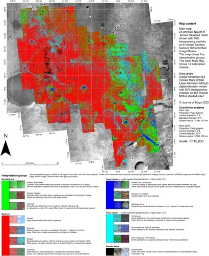
Table 1. Hierarchical classification system consists of 14 descriptive classes, divided into 5 interpretive groups.

Note: For more detail on how this classification system was developed and applied, see Barrett et al. (2022).

Seven of the descriptive classes comprise continuous surfaces, encompassing different roughness grades. The remaining classes cover dispersed landforms, with six describing different bedform morphologies and one covering boulder fields. The five Interpretive Groups consist of: Non-Bedrock Surfaces, Bedrock Surfaces, Large Ripples, Small Ripples, and Boulder Fields. Thus, the smoother classes (lacking evidence for fractures or resolvable sharp-edged textures) are interpreted as non-bedrock, while the rougher classes are believed to be bedrock. The ripple classes are divided according to size. Type examples are presented in the legends to the two main map sheets, and a more detailed description of the classes has been published in Barrett et al. (2022), figures 1 and 2 of that paper present a wider variety of type examples, anotating how the different classes are defined.

Examples of these features were labelled manually in 1504 small sections of HiRISE images. A detailed description of this procedure can be found in Barrett et al. (2022) where figures six and seven of that paper show the labelling process. Each of these ‘framelets’ was 128 × 128 m in size. Features were labelled at a pixel scale, by drawing a polygon around the set of pixels which all conformed to a given class. This was then converted to raster data and used to train the model. Most framelets contained examples of multiple features, and we aimed to provide a representative variety of combinations.

This dataset was used to train the DL network. The model learnt to recognise and segment the ontological classes, applying the scheme over entire HiRISE images in a fraction of the time it would have taken for a human expert to manually map the site. Classification was conducted on a pixel scale, using a much smaller moving window than the size of the training framelets. The output consists of a coloured raster, where each pixel has been assigned a class. There was no ‘background’ or ‘no class’ colour rather, the closest of the 14 classes was assigned.

Forty-nine publicly available HiRISE images of the Oxia Planum landing site were used as the input for NOAH-H (Table S1). Relatively little pre-processing was required. The aim was to produce a system where any HiRISE image could be downloaded from the Planetary Data System and classified with relatively few steps. For many purposes, it would have been preferable to make a carefully controlled mosaic, where only images with consistent emission angles were used. These could then be normalised and corrected for atmospheric conditions. The end product might be improved, however, there is then the risk that the final DL model is only suitable for use with images that have been similarly controlled. Instead, we elected to select images with a variety of conditions, so that our training dataset would be as generic as possible and thus transferable to as many images as possible. Using uncontrolled images was not expected to have a substantial impact on the end result.

HiRISE images are not accurately georeferenced, resulting in classification products that match their source HiRISE image but do not line up exactly with any given basemap. Georeferencing the classified rasters would be challenging since landmarks cannot easily be recognised in them. Instead, we georeferenced the source HiRISE image and then applied the same control points and transformations to the NOAH-H raster. Since the area and pixel size of the two products is identical, this precisely co-registers the classified raster, allowing for future manipulation using Geographic Information Systems (GIS). This procedure is outlined in Wright et al., (2022). A mosaic of 6 m/pixel context camera (CTX) images (Malin et al., 2007) was used as the co-registration base for the HiRISE images. This was produced at the London Natural History Museum as described in Fawdon et al. (2021), and is controlled to High-Resolution Stereo Camera (HRSC) images. The CTX mosaic was used to place a trigonal grid of control points across each HiRISE image using ArcGIS Pro 2.8. Where possible, control points were preferentially placed on already co-registered HiRISE images. Where this was not possible, the CTX mosaic was used. Spline transformations were applied to each HiRISE image so that each control point was co-registered exactly with the target mosaic.

In cases where co-registered rasters overlap, there was some variability in the classification due to subtle variations in the source images (e.g. lighting angle, spacecraft pointing angle, time of year). It was found that broad trends remained consistent regardless of which source image was classified, however, there were pixel scale variations that needed to be accounted for.

To do this, and to control which pixels ended up in the final mosaic, a priority order was determined. The descriptive classes were ranked, with the most accurately identified being prioritised. This was determined using the Precision, Recall, and Intersection over Union (IoU) metrics discussed in Barrett et al. (2022). Classes that exhibited a higher perceived hazard for traversability assessment were also ranked more highly than safer classes, using the qualitative hazard assessments presented in Barrett et al. (2022) and in Table 1. Each accuracy metric was used to generate a ranking from 1 to 14, with more highly ranked values being assigned a higher score than those ranked lower. The hazard assessments were also converted into scores from 1 to 7. These scores were summed to determine an overall mosaic pixel priority for each class. The ranking is shown in Table 2. A similar procedure was employed to rank the interpretive groups. Here hazard varies within each group, and so this metric was omitted. Instead, in cases of conflicts, dispersed features such as bedforms and boulder patches were prioritised over surfaces. The ranking is shown in Table 3.

Table 2. Considerations used during the process of determining priority of the different classes in areas where the classified rasters overlap.

Class number	Descriptive class	Ranked priority score	Type	Hazard rating score	Recall	Precision	Mean IoU
10	Large ripples – rectilinear	14	Distributed	7	83	100	82
7	Bedrock – fractured	13	Surface	4	86	88	76
8	Large ripples – simple form, continuous	12	Distributed	6	86	80	70
14	Boulder fields	11	Distributed	4	84	85	73
6	Bedrock – rugged	10	Surface	7	85	81	70
9	Large ripples – simple form, isolated	9	Distributed	5	70	70	53
2	Non-bedrock – smooth, lineated	8	Surface	6	69	73	54
3	Non-bedrock – textured	7	Surface	2	67	74	54
11	Small ripples – continuous	6	Distributed	6	64	63	46
13	Small ripples – non-continuous – non-bedrock substrate	5	Distributed	5	63	71	50
4	Bedrock – smooth	4	Surface	1	66	57	44
12	Small ripples – non-continuous – bedrock substrate	3	Distributed	4	51	33	25
5	Bedrock – textured	2	Surface	4	49	55	34
1	Non-bedrock – smooth, featureless	1	Surface	2	60	47	35

Note: Classes are ranked in descending order of priority.

Table 3. Considerations for ranking the priority of the interpretive groups.

#	Interpretive group	Ranked priority	Type	Recall	Precision	Mean IoU
3	Large ripples	5	Distributed	90	89	80
4	Small ripples	4	Distributed	75	76	60
5	Boulder fields	3	Distributed	85	85	73
2	Bedrock	2	Surface	97	98	94
1	Non-bedrock	1	Surface	96	95	90

The mosaic was created in ArcGIS Pro, using the ‘Lookup’ and ‘Mosaic to New Raster’ tools. The ‘Mosaic Operator’ parameter was set to ‘maximum’ so that the pixels with the highest priority were included in the final mosaic whenever pixel classification conflicts occurred.

4. Results

The final iteration of the neural network produced reliable results, which showed good agreement with human labelled validation areas. The model exhibited a mean IoU of 74.15% for the descriptive classes, and 92.33% for the interpretive groups (Barrett et al., 2022). This suggests that the model output is fit for purpose. Figure 2 shows a comparison of a classified area with the original HiRISE image.

Since ExoMars Rosalind Franklin has yet to land, it is not yet possible to verify the ‘ground truth’ at the site and confirm that the model predictions match the in situ environment. However, NOAH-H has also been applied to HiRISE images of Jezero Crater, the landing site for NASA’s Mars 2020 Mission. Comparison of NOAH-H classification with in situ images from Perseverance Rover and Ingenuity Helicopter shows that the model output can be reliably matched with in situ images and that the same transitions between ontological classes are visible on the ground. Comparison with pre-existing geomorphological maps of the Jezero site has also demonstrated good agreement when landscape-level trends are considered (see; Table 4 and Figure 6 Wright et al., 2022). As the ExoMars mission advances, it will become possible to conduct similar investigations at the Oxia Planum site, where the model was trained.

Figure 3 shows the main map sheet 1, and the distribution of descriptive classes across the site. Figure 4 shows the same area, but with the classes combined into interpretive groups. This data is available in supporting online materials for study in GIS. There are a few very small data gaps, since the images had to be cropped slightly in order to remove an edge effect in the classification. This has left a few ‘seams’ in the images, where the adjacent HiRISE images do not quite touch. Fortunately, data gaps are relatively small in this area, due to extensive overlapping HiRISE coverage collected for the ExoMars landing site characterisation process. Slight differences in quality between HiRISE images also sometimes result in breaks in the classification, where one class is more prevalent in one image than another. Otherwise, the result is generally very consistent across the classified area.

5. Applications of the classified mosaic

The mosaic can be used to automate various tasks which would otherwise require intensive manual input. To illustrate this, six classes covering different aeolian bedform morphologies are considered. These classes describe Transverse Aeolian Ridges (TARs; Balme et al., 2008). TARs are metre to decametre scale granular ripple-like bedforms found on the surface of Mars (Balme et al., 2008). They form transverse to the prevailing wind direction, and since most are immobile in the modern day, preserve information about the paleo-wind regime under which they formed. They are believed to form in a similar manner to terrestrial megaripples (Zimbelman & Foroutan, 2020) and are likely an analogous landform. Movement has recently been observed in megaripples in the North Polar Erg of Mars (Chojnacki et al., 2021).

Results for the aeolian bedform classes were found to be very reliable. Large ripples had a Recall statistic of ∼90% when compared to manually labelled areas (Barrett et al., 2022). This suggests that relatively few features were missed by the model when identifying this group of classes. The Precision statistic was also around 90% indicating that false positives were rare and that most features identified as large ripples by the model did conform to this class. Confusion occurred within the large ripple group rather than between it and the other groups. This means the model output can reliably be used to calculate ripple density statistics across the entire classified area, a process that would normally require extensive manual mapping.

TAR density maps were produced using ArcGIS. A 1 km² grid, based on that of Fawdon et al. (2021), was clipped to the classified area. The classified mosaic of Descriptive Classes was down-sampled to 1 m per pixel so that number of pixels could more easily be equated with the area. This did not adversely affect the classification, as most variations in texture occur on a decametre scale. Each individual ripple class was then extracted, producing a set of binary masks describing the presence or absence of that class for each pixel. This was done for each of the six bedform classes and several combinations of classes; all ripple classes (classes 8–13), all large ripples (classes 8–10), all small ripples (classes 11–13), all continuous ripples (classes 8–11) and all discontinuous ripples (classes 12–13).

The plots for large and small ripple classes show the respective interpretive groups. Continuous ripples are defined as those classes where the classified pixels do not include any non-ripple material between them. Somewhat counterintuitively, this includes large isolated ripples, since only the ripple itself is classified and all non-ripple material is excluded from the pixels predicting this class. In the case of classes 12 and 13, the classification returns an area where small ripples predominate but are not continuous. We estimate that they have approximately 20% coverage in these classified areas, with the remainder comprising either a bedrock or non-bedrock substrate. Actual TAR density in areas classified as classes 12 and 13 are thus somewhat lower than the density of areas classified as other classes.

For each of these products, the ‘add surface information’ tool in ArcGIS was used to compute bedform density for each 1 km grid ‘quad’ square. This tool summarises a specified value in a raster over an area bounded by a vector feature. In this case, the proportion of pixels classified as ripples of each type was calculated for each quad using a ‘mean’ operation. The result was a 1 km square output grid which can be symbolised to show variations in TAR density across the study area. This procedure could be applied to any of the 14 ontological classes. Aeolian hazards are very important for landing site characterisation, as are areas with dense boulder fields, or large expanses of rugged bedrock terrain.

These maps provide more nuanced information about the type and extent of TAR coverage than is available from the main mosaics. Areas of high TAR density, coloured in reds and oranges, are immediately apparent. These are regions that should be avoided when placing landing ellipses or planning rover routes. The density maps show the distribution of sink areas for aeolian material. These are generally found in areas of low-lying topography such as the floors of impact craters, and the valleys left behind by paleo-river systems. The greatest density of TARs is found on the floor of the South Neocoogoon Vallis in the south-eastern region of the landing site (Fawdon et al., 2021), and around a subtle north-south trending valley in the far east of the site. Other strong signals are seen from the largest impact craters to the south and west. The density maps also highlight the presence of extensive fields of small TARs, which are more prevalent outside of impact structures than their larger equivalents. These features produce a large number of quads with greater than 25% TAR density.

These density maps highlight hazardous areas which would not be apparent from a study of the site’s topography alone. However, comparison with elevation data provides increased insight into these results. Concentrations of TARs tend to occur in shallow depressions of various types. Such areas would not be obvious from a manual inspection of the red band HiRISE images. A large area to the west of the landing site has relatively low TAR coverage, appearing blue (0–5% coverage) in the density maps. This area corresponds to a specific morpho-stratigraphic unit that is elevated relative to its surroundings. Slight depressions on the surface here have slightly elevated TAR density, appearing yellow (5–10% coverage) on the maps. Further geological mapping of this site could highlight which geological units are the best sources of windblown material, as well as the best sinks.

Producing the same results manually would have required substantially more work. For example, the TAR statistics in Favaro et al. (2021) were primarily based on manual mapping by a team of scientists. Compiling that dataset took approximately 350 person-hours of work, manually digitising TARs over an area comparable to the size of the mosaic presented herein. Extending that manual digitisation to a larger area would require a proportionally increased effort. By comparison, the labelling campaign for the entire NOAH-H study (i.e. detailing many more classes than just the TARs) was conducted in approximately 270 person-hours. Although the person-time overhead required before data collection can begin is high, extending the study to larger areas takes almost no extra time demonstrating the advantage of using this DL approach.

6. Discussion

Now that the DL system is trained, it can easily be applied over as large an area as needed. Georeferencing the resulting classification products becomes the most time-consuming part of the process but can be mitigated by pre-mosaicking and tiling before the DL step is applied. The pay-off for using the machine learning approach becomes greater the larger the area that is studied, as the training and labelling effort becomes a proportionally smaller part of the effort.

Every effort was made to keep the surface textures as generic as possible, so that the classification scheme would be applicable to as wide an area as possible. However, sites with landforms that are not present in Oxia Planum exhibit more misclassifications. Features like dark dunes or transitional ripple morphologies have been seen to cause confusion at other sites (Wright et al., 2022). Sites where only a limited selection of the 14 classes are present should perform fine, however, if there are more than one or two new features that do not fit into the existing ontology then the model may struggle to provide a useful classification for those features. If the system were to be applied more generally to other sites, then comparative work would need to be done to identify the gaps in the classification scheme with application to a specific geographic region or intended science question. Additional labelling work could then be undertaken to fill in the relevant gaps in the classification.

This technique has great potential to aid in the mapping of similar areas. The application of DL-driven classification massively speeds up the process of classifying planetary surfaces. While this system cannot replicate the process by which a human would produce a morphostratigraphic map, it nonetheless provides a richer data product that the human mapper can use to inform such efforts. The production of density maps like those presented in Figures 5 and 6 rapidly provides the user with both quantitative and qualitative information about the prevalence of their chosen classes. Density maps can easily be used to generate statistics such as those in Figure 7. We anticipate tools of this sort to become increasingly common, as they allow a relatively small amount of classification work to be conducted in a feasible time scale, but then extrapolated by DL over an area that would be impossible to survey by hand.

Figure 5. Dispersed feature density map for (a) all ripple classes and (b) all boulder fields. An indicative landing ellipse for the ExoMars rover mission is overlain on all maps. This landing ellipse describes a 2022 launch opportunity and will differ from the eventual ExoMars landing ellipse. Map centred on 18.1°N 24.2°W.

Two maps of the classified area show the gridded density of Ripples, and Boulders respectively. The central area of the landing site has the lowest ripple density, it is highest in the east, with medium density squares to the north. Boulders have much lower density than ripples, only occurring densely in an area classified from a single higher quality image.

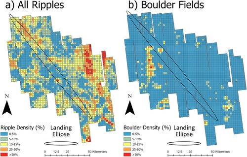
Figure 6. TAR density map for thematic groups. (a) Large ripples (classes 8–10), (b) small ripples (classes 11–13), (c) ‘continuous’ ripples (classes 8–11), (d) discontinuous ripples (classes 12–13). We considered weighting plot d to reflect that only 20% of pixels classified as discontinuous ripples are estimated to be the ripples themselves, with the remaining 80% being non-ripple material between the TARs. However, doing so produced a plot where every grid square was <10% and all but two were <5%. The result showed no useful distribution data. An indicative landing ellipse for the ExoMars rover mission is overlain on all maps. This landing ellipse describes a 2022 launch opportunity and will differ from the eventual ExoMars landing ellipse. Map centred on 18.1°N 24.2°W.

Four gridded density maps break down the ripple distribution further. All show similar spatial distributions, with the main difference being density. Discontinuous ripples have the lowest density, with relatively few squares showing 1–2.5%. Continuous ripples are far more common. Small ripples are much more prevalent than large ripples, though very dense examples of both are rare.

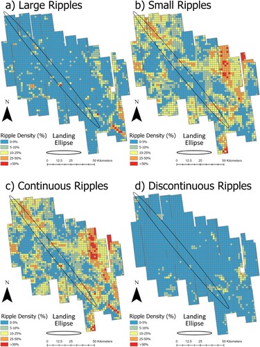
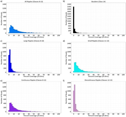
Figure 7. Histograms summarising the density information presented in Figures 5 and 6 (a) All ripples (classes 8–13) (b) boulders (class 14), (c) large ripples (classes 8–10), (d) small ripples (classes 11–13), (e) continuous ripples (classes 8–11), (f) discontinuous ripples (classes 12–13). Each plot shows percentage coverage, divided into 2% bins. Quads are 1 km². Note the difference in scale between boulders and ripple classes due to the very large number of quads with little to no boulder cover.

Boulders are shown to have a far lower percentage coverage than any of the ripple classes, with a count of >2200 in the ‘0’ bin. Large ripples and discontinuous ripples have similar distributions, weighted heavily to the lower bins, with a very small tail. Continuous and Small ripples have a similar distribution to all ripples, with a peak around five for continuous and around 1 for small. They trail off at higher percentage coverage, which is a curve approximating an exponential decrease.

The system was developed with several use cases in mind. Foremost of these was traversability assessment for the upcoming ExoMars mission. The classes are designed to form one input to a formal route planning exercise, when compared with the engineering capabilities of the rover as determined through field trials and in situ evidence from rover cameras. Consequently, the distinctions in texture are those which are expected to be most significant for such an exercise. For example, the cut-off between small and large ripples was chosen with the intent that small ripples are those which could likely be crossed by a rover, while large ones would be impediments to travel. The two main map products are intended to be used as a starting point for more in-depth mapping and hazard assessment once the ExoMars rover lands. Quantifying the density of aeolian and clastic cover is an important part of determining both where the rover can safely land, and in which directions it should attempt to traverse. The prevalence of rugged bedrock could also be of use, especially as the rugged bedrock class can identify the rugged rims of small impact craters with good fidelity.

These results are also being used to characterise the aeolian history of Oxia Planum, helping the authors to identify and digitise bedforms of different morphologies over the large areas required (Favaro et al., 2021). Data on bedform distribution can then be compared with other relict landforms, modelling data, and the directionality of modern dust devil tracks to better understand how the aeolian environment changes over time. Other potential applications include quantifying boulder distribution around impact craters. Density statistics of the sort presented here will be most useful for this latter case, as the prevalence of boulder, or ripple, covered ground can be quantified on a smaller scale to explore how the distribution of aeolian and clastic cover responds to other controls such as topography and emplacement onto bedrock vs non-bedrock surfaces. On the technical side further work will include testing the model on orthorectified stereo images, where we can examine the difference in classification between overlapping pixels and produce statistics for reproducibility when different images are classified (as in the overlapping areas of this and other mosaics.)

7. Conclusions

NOAH-H was used to produce a 25 cm/pixel terrain map of the ExoMars landing site in Oxia Planum, Mars. The system produced useful maps of the site, which are already aiding human mappers in understanding both the aeolian history of the landing site (Favaro et al., 2021) and its geology (Fawdon, Orgel, et al., 2022). We show how the map can be translated into gridded statistics on bedform abundance, an important consideration for both selection of and navigation within a landing site.

Software

We used ESRI ArcGIS Pro 2.8 for co-registration of HiRISE and NOAH-H rasters, NOAH-H pixel prioritisation, and generation of the NOAH-H terrain classification map. NOAH-H is a deep learning semantic segmentation software developed by SciSys Ltd (now part of CGI) for the European Space Agency to aid preparation for the ExoMars rover mission.

Acknowledgements

The HiRISE images discussed in this work are publicly available from https://www.uahirise.org/ and are credited to NASA/JPL/University of Arizona.

Disclosure statement

No potential conflict of interest was reported by the author(s).

Data availability statement

The georeferenced mosaics and feature density plots are available from the Open University’s Open Research Data Online (ORDO) system: NOAH-H Mosaics: DOI 10.21954/ou.rd.19802695 and Gridded density Statistics: DOI 10.21954/ou.rd.19802626.

Correction Statement

This article has been corrected with minor changes. These changes do not impact the academic content of the article.

Additional information

Funding

AMB, JW and MRB acknowledge funding from the UK Space Agency and UK Science and Technology Facilities Council (STFC; grant ST/T000228/1), and a European Space Agency contract (4000118843/16/NL/LvH1145 – Novelty or Anomaly Hunter (NOAH)). EAF and MRB gratefully acknowledge UK Space Agency (UK SA) funding [grant numbers ST/T002913/1, ST/V001965/1 and ST/R001413/1]. PF acknowledges UK SA funding [grant numbers ST/V001965/1 and ST/R001413/1].

References

- Balme, M., Berman, D. C., Bourke, M. C., & Zimbelman, J. R. (2008). Transverse aeolian ridges (TARs) on Mars. Geomorphology, 101(4), 703–720. https://doi.org/10.1016/j.geomorph.2008.03.011
- Barrett, A. M., Balme, M. R., Woods, M., Karachalios, S., Petrocelli, D., Joudrier, L., & Sefton-nash, E. (2022). NOAH-H, a deep-learning, terrain classification system for Mars: Results for the ExoMars Rover candidate landing sites. Icarus, 371(September 2021), 114701. https://doi.org/10.1016/j.icarus.2021.114701
- Chojnacki, M., Vaz, D. A., Silvestro, S., & Silva, D. C. A. (2021). Widespread megaripple activity across the north polar ergs of Mars. Journal of Geophysical Research: Planets, 126(12), 1–19. https://doi.org/10.1029/2021JE006970
- Favaro, E. A., Balme, M. R., Davis, J., Grindrod, P. M., Fawdon, P., Barrett, A. M., & Lewis, S. R. (2021). The aeolian environment of the landing site for the ExoMars Rosalind Franklin rover in Oxia Planum. Mars. Journal of Geophysical Research (Planets), 126(4), e2020JE006723. https://doi.org/10.1029/2020JE006723.
- Fawdon, P., Balme, M., Davis, J., Bridges, J., Gupta, S., & Quantin-Nataf, C. (2022). Rivers and lakes in western Arabia terra: The fluvial catchment of the ExoMars 2022 rover landing site. Journal of Geophysical Research: Planets, 127(2), e2021JE007045https://doi.org/10.1029/2021JE007045.
- Fawdon, P., Grindrod, P., Orgel, C., Sefton-Nash, E., Adeli, S., Balme, M., Cremonese, G., Davis, J., Frigeri, A., Hauber, E., Le Deit, L., Loizeau, D., Nass, A., Parks-Bowen, A., Quantin-Nataf, C., Thomas, N., Vago, J. L., & Volat, M. (2021). The geography of Oxia Planum. Journal of Maps, 17(2), 621–637. https://doi.org/10.1080/17445647.2021.1982035
- Fawdon, P., Orgel, C., Sefton-Nash, E., Adeli, S., Balme, M., Davis, J., Frigeri, A., Grindrod, P., Hauber, E., Le Deit, L., Loizeau, D., Nass, A., Quantin-Nataf, C., Volat, M., de Witte, S., Vago, J. L., & the ExoMars RSOWG ‘Macro’ Group. (2022). The reconciliation of HiRISE scale mapping at Oxia Planum: The landing site for the ExoMars Rosalind Franklin rover. 53rd Lunar and Planetary Science Conference, 2210, 2.
- Malin, M. C., Bell, J. F., Cantor, B. A., Caplinger, M. A., Calvin, W. M., Clancy, R. T., Edgett, K. S., Edwards, L., Haberle, R. M., James, P. B., Lee, S. W., Ravine, M. A., Thomas, P. C., & Wolff, M. J. (2007). Context camera investigation on board the Mars reconnaissance orbiter. Journal of Geophysical Research, 112(E5), E05S04. https://doi.org/10.1029/2006JE002808
- McEwen, A. S., Eliason, E. M., Bergstrom, J. W., Bridges, N. T., Hansen, C. J., Delamere, W. A., Grant, J. A., Gulick, V. C., Herkenhoff, K. E., Keszthelyi, L., Kirk, R. L., Mellon, M. T., Squyres, S. W., Thomas, N., & Weitz, C. M. (2007). Mars reconnaissance orbiter’s high resolution imaging science experiment (HiRISE). Journal of Geophysical Research E: Planets, 112(5), 1–40. https://doi.org/10.1029/2005JE002605
- McNeil, J. D., Fawdon, P., Balme, M. R., & Coe, A. L. (2021). Morphology, morphometry and distribution of isolated landforms in southern Chryse Planitia, Mars. Journal of Geophysical Research: Planets, 126(5), e2020JE006775https://doi.org/10.1029/2020JE006775.
- Poulet, F., Gross, C., Horgan, B., Loizeau, D., Bishop, J. L., Carter, J., & Orgel, C. (2020). Mawrth Vallis, Mars: A fascinating place for future in situ exploration. Astrobiology, 20(2), 199–234. https://doi.org/10.1089/ast.2019.2074
- Quantin-Nataf, C., Carter, J., Mandon, L., Thollot, P., Balme, M., Volat, M., Pan, L., Loizeau, D., Millot, C., Breton, S., Dehouck, E., Fawdon, P., Gupta, S., Davis, J., Grindrod, P. M., Pacifici, A., Bultel, B., Allemand, P., Ody, A., … Broyer, J. (2021). Oxia Planum: The landing site for the ExoMars “Rosalind Franklin” rover mission: Geological context and prelanding interpretation. Astrobiology, 21(3), 345–366. https://doi.org/10.1089/ast.2019.2191
- Summons, R. E., Amend, J. P., Bish, D., Buick, R., Cody, G. D., Des Marais, D. J., Dromart, G., Eigenbrode, J. L., Knoll, A. H., & Sumner, D. Y. (2011). Preservation of Martian organic and environmental records: Final report of the Mars biosignature working group. Astrobiology, 11(2), 157–181. https://doi.org/10.1089/ast.2010.0506
- Vago, J. L., Westall, F., Coates, A. J., Jaumann, R., Korablev, O., Ciarletti, V., Mitrofanov, I., Josset, J. L., De Sanctis, M. C., Bibring, J. P., Rull, F., Goesmann, F., Steininger, H., Goetz, W., Brinckerhoff, W., Szopa, C., Raulin, F., Edwards, H. G. M., Whyte, L. G., … Carreau, C. (2017). Habitability on early Mars and the search for biosignatures with the ExoMars rover. Astrobiology, 17(6–7), 471–510. https://doi.org/10.1089/ast.2016.1533
- Wright, J., Barrett, A. M., Fawdon, P., Favaro, E., Balme, M. R., Woods, M. J., & Karachalios, S. (2022). Jezero Crater, Mars: Application of the deep learning NOAH-H terrain classification system. Journal of Mapshttps://doi.org/10.1080/17445647.2022.2095935.
- Zimbelman, J. R., & Foroutan, M. (2020). Dingo gap: Curiosity went up a small transverse aeolian ridge and came down a megaripple. Journal of Geophysical Research: Planets, 125(12), 1–16. https://doi.org/10.1029/2020JE006489