Mapping population distribution from open address data: application to mainland Portugal

ABSTRACT

Mapping population distribution remains a common need in various fields of studies. Several approaches and methodologies have been adopted to obtain high-resolution population distribution grids. The use of addresses data to obtain gridded population distribution maps emerges as one of the more recent and accurate approaches. The increasing dissemination and availability of geo-data and more specifically address data allow us to obtain updated, granular and high spatial resolution population distribution maps. This paper describes a bottom-up open addresses data mapping-based approach of gridded population distribution with a fine spatial resolution. Through a QGIS plugin, an adaptation of the housing unit methodology was implemented to obtain 500 m × 500 and 250 m × 250 m population grids for mainland Portugal. The results showed that the use of reliable addresses databases can generate gridded population distribution maps with a high degree of adjustment to reality.

KEYWORDS:

• Population distribution
• grid map
• addresses
• open data

1. Introduction

The population distribution mapping remains essential in geographic studies, enabling the understanding of various human-environment interrelationships and practices.

Although some countries provide gridded population data, typically the population distribution can be found in vector format through administrative units or census enumeration units. Gridded population counts offer several significant advantages over irregular zones (Lloyd, Sorichetta, et al., 2017). Martin et al. (2011) indicate as advantages of gridded population models the stability through time and ease of integration with other georeferenced data sources from environmental, physical, or social applications.

Regarding the various existing approaches to map the population distribution, Calka et al. (2017) differentiate them according to the techniques (disaggregation or aggregation), the mapping unit, the ancillary data used or the visualization methods. As stated by Wardrop et al. (2018), for a given spatial unit, population distribution grids can be produced by disaggregating (e.g. gridding) population counts (top-down approach) or by estimating that count at the grid cell level by combining sampling with ancillary data (bottom-up method). Regardless of the approach used to map population distribution, the objective of accounting for the population with the greatest possible precision is always present. In this context, Gallego (2010) refers to the collection of individual data with coordinates of the dwellings and counting the number of people in each cell of the grid (bottom-up approach) as the best way to produce the gridded map of population density. Martin et al. (2011) reinforce this approach, describing that the most promising results in gridded population models are obtained with the most detailed centroid locations, in which each centroid represents the location of a single individual or household in the population, and no redistribution modelling would be required.

This paper develops a bottom-up applied methodology approach to produce a gridded population distribution map with a fine spatial resolution (i.e. 500 m × 500 m and 250 m × 250 m) from open addresses data. Supported by a government address open data, a methodology for creating raster layers with different resolutions for Portugal’s mainland is proposed. The distinguishing feature of this study for the approaches that aggregate households is that the address data is supported by open government data and does not have any resident population counting, constituting a novelty in the Portuguese context. Combining open addresses data with the census, increases the spectrum of use for this data in census mapping, particularly in topics like the before and after population mapping using censuses and administrative sources or transition and evolution in population mapping.

The aggregation of addresses for obtaining population distribution grids is an approach tested in different ways. For example, Norman et al. (2003) use household counts for each postcode whereby the number of postcode centroids in an area of overlap between source and target zones is used to determine the proportion of the source zone population to be allocated to the zone of intersection. In 2010, Eurostat launched the ESSnet project ‘GEOSTAT – representing census data in a European population grid dataset’ taking advantage of the 2011 Census (GEOSTAT, 2011). This project geocoded various population characteristics into a 1 km² grid dataset using disaggregation and aggregation algorithms. In Portugal, the availability of the georeferenced 2011 census buildings Portugal allowed to determine the exact population within each grid cell for the 2011 census (GEOSTAT, 2011) using an aggregation approach. Previous research has shown that postcodes are a proxy for population density and therefore provide a suitable basis for reallocating population counts (Lloyd, Catney, et al., 2017). Bakillah et al. (2014) present a method for areal interpolation at the building level that uses VGI as ancillary data. As stated by the authors (Bakillah et al., 2014), the principle of the approach is to combine three existing methods: multi-class dasymetric mapping to obtain population estimates for relatively large zones; then, interpolation by surface volume integration; and finally, binary dasymetric mapping is used to redistribute population within buildings. Based on the assumption that housing space is a proxy for the number of its residents, Biljecki et al. (2016) estimated the Netherlands population with 3D city models using census and building data. Schug et al. (2021) mapped gridded population across Germany using weighting layers from building density, building height, and building type datasets, based on Copernicus Sentinel-1, Sentinel-2 data, as well as from crowd-sourced OSM data. More recently, Tu et al. (2022) generated high-resolution gridded population data for China from digital footprint and ancillary geospatial data.

The remainder of the paper comprises four sections. In Section 2 we review the study area, the data used for the analysis and the bottom-up mapping-based approach applied to build the gridded population distribution maps; and Section 3 is about the implementation and comparison between model outputs for different resolutions and true population counts are presented, for methodology validation. In Section 4, the model performance, geographical context, and data are discussed.

2. Materials and methods

2.1. Study area

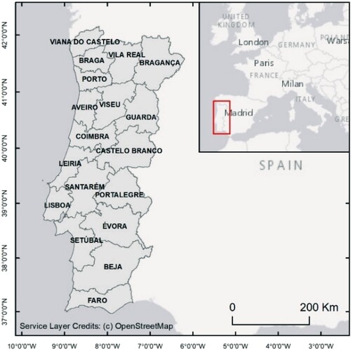
The method proposed in this study was applied on Portugal mainland (Figure 1). Portugal mainland is in the southwest of Europe (between latitudes 33° and 43° N, and longitudes 32° and 6° W), with a total land area of approximately 89,015 km². With approximately 10.3 million residents at the end of 2021, Portugal is the 11th most populated country in Europe.

Figure 1. Portugal mainland location.

Map of Portugal mainland including districts. Small map of Europe with Portugal mainland location.

2.2. Data

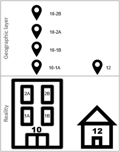
In this study, the number of housing units is based on the administrative layer of addresses, for the year 2011, obtained from the INSPIRE ATOM download service of the Portuguese National Statistics Institute (INE) Geographic Data Set. This data set is structured in accordance with the INSPIRE Directive, Annex I, Addresses theme.¹ The data obtained from the INSPIRE ATOM download service resulted in 278 files (GML format) in the PTM06-ETRS89 reference system (EPSG: 3763). The 278 data sets, materialized in a point layer, present for each record the building number, the floor and the flat/apartment number/identification (Figure 2).

Figure 2. Point layer example with address data for two buildings.

Image of one building with one address and image of another building with four addresses and the correspondent point layer representation.

To have a single layer for mainland Portugal, these files were merged into a single shapefile with 5,669,971 records.

The average number of people per housing unit was obtained from the statistical subsections of the Geographic Information Referencing Base (BGRI), referring to the 2011 Census, available on the INE website.²

2.3. Methodology

2.3.1. Population estimation

To calculate the gridded resident population, an adaptation of the housing unit methodology was used. The housing unit method assumes that most people live in any type of housing structure (Deng et al., 2010), according to the following formula: (1) $P_t=\left(A_t\times \mathrm{M}\mathrm{P}{\mathrm{A}}_t\right)+\mathrm{O}{\mathrm{P}}_t$(1) where P_t is the population at time t, A_t is the number of dwellings occupied at time t, MPA_t is the average number of people per accommodation at time t and OP_t corresponds to other people who do not live in any type of traditional housing structure (e.g. homeless).

The sequence of procedures for calculating the resident population on a grid surface is summarized in the flowchart of Figure 3.

Figure 3. Flowchart for calculating the population on a grid.

Step by step GIS functions used to calculate population grid.

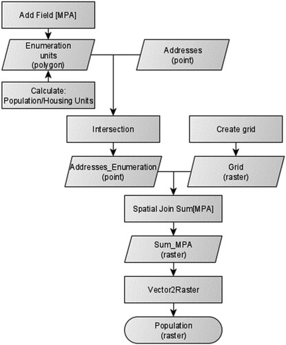
The first step in the workflow consists of adding a field (MPA) in the census enumeration layer. This field is used in the next step to calculate the average resident population per housing unit. The third step refers to the intersection of the point addresses layer, with the polygons of the census enumeration layer to identify to which statistical area each housing unit belongs to. In the fourth step, a vector grid is created with a width and height corresponding to the raster resolution. The next step consists of the vectorial junction between the addresses layer and the grid, wherein each record the value of the average resident population per housing unit is added, obtaining the resident population in each vector unit. The last step is the vector grid to a raster layer conversion.

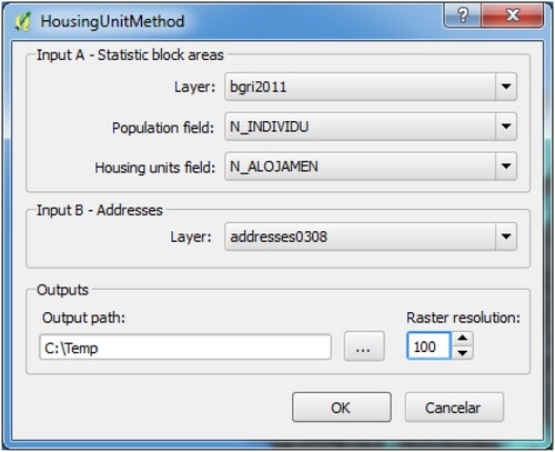
To automate the process of calculating the resident population on a grid, a plugin was developed for QGIS desktop software. The QGIS plugin interface selects the layer of the statistical subsections, the fields referring to the resident population and number of housing units, the layer of housing units/addresses and the path of the folder to store the results (Figure 4).

Figure 4. QGIS plugin interface.

Image of QGIS plugin interface used to calculate population grids.

2.3.2. Accuracy assessment

Three error measurements were employed in this study, the mean absolute error (MAE) (Equation (2)), the: Root Mean Square Error (RMSE) (Equation (3)) and mean algebraic percentage error (MALPE) (Equation (4)): (2) $\mathrm{M}\mathrm{A}\mathrm{E}={\displaystyle \frac{1}{n}\sum _{i=1}^n\left|{\hat{P}}_i-P_i\right|}$(2) (3) $\mathrm{R}\mathrm{M}\mathrm{S}\mathrm{E}=\sqrt{{\displaystyle \frac{{\sum }_{i=1}^n{\left({\hat{P}}_i-P_i\right)}^2}{n}}}$(3) (4) $\mathrm{M}\mathrm{A}\mathrm{L}\mathrm{P}\mathrm{E}=100\text{\%}\times {\displaystyle \frac{1}{n}\sum _{i=1}^n{\displaystyle \frac{{\hat{P}}_i-P_i}{P_i}}}$(4) where ${\hat{P}}_i$ is the estimated value for population, P_i is the actual value for population obtained from 2011 Census and n is the total number of cells. MAE and RMSE are measures of precision, reflecting how close the estimated values are to the actual values, while the MALPE is a measure of bias, focusing on whether the total estimate shows an upward or downward tendency (Smith et al., 2002; Smith & Cody, 1994).

3. Results

3.1. Population by district

The estimated total Portuguese mainland population for the 500 m (Table 1) and 250 m (Table 2) resolution grids revealed an underestimation (−1.9% and −1.3%) when compared to the total population in the census grids. The two most populated districts, Lisboa and Porto, also underestimate the estimated population: in the 500 m model the results were −2.6% and −2.1%, respectively, and in the 250 m model results were −2.4% and −1.9%, also respectively. In the opposite direction, the district of Faro has an overestimation, for the total population for resolution of 250 and 500 m, of +3.9% and +5.7%, respectively.

Table 1. 500 m resolution model and actual population by district.

District	Model 500 m	Census 500 m	Δ (%)
Aveiro	697,573	712,422	−2.1
Beja	148,980	148,376	0.4
Braga	831,137	847,674	−2.0
Bragança	134,303	135,046	−0.6
Castelo Branco	193,289	193,653	−0.2
Coimbra	426,671	427,935	−0.3
Évora	163,065	164,506	−0.9
Faro	463,149	445,563	3.9
Guarda	155,579	158,825	−2.0
Leiria	454,555	468,654	−3.0
Lisboa	2,187,147	2,245,188	−2.6
Portalegre	114,948	116,551	−1.4
Porto	1,774,625	1,812,763	−2.1
Santarém	439,084	450,882	−2.6
Setúbal	820,457	845,881	−3.0
Viana do Castelo	237,710	243,883	−2.5
Vila Real	203,224	204,854	−0.8
Viseu	365,404	375,660	−2.7
Total	9,810,900	9,998,316	−1.9

Table 2. 250 m resolution model and actual population by district.

District	Model 250 m	Census 250 m	Δ (%)
Aveiro	697,899	710,110	−1.7
Beja	149,288	146,647	1.8
Braga	830,129	843,203	−1.6
Bragança	134,246	133,393	0.6
Castelo Branco	193,291	190,208	1.6
Coimbra	426,996	424,813	0.5
Évora	163,172	163,031	0.1
Faro	464,705	439,557	5.7
Guarda	155,571	156,241	−0.4
Leiria	454,634	463,696	−2.0
Lisboa	2,189,043	2,243,040	−2.4
Portalegre	114,969	115,129	−0.1
Porto	1,778,228	1,813,325	−1.9
Santarém	438,717	444,827	−1.4
Setúbal	822,392	844,693	−2.6
Viana do Castelo	238,009	241,453	−1.4
Vila Real	203,509	202,480	0.5
Viseu	365,296	370,818	−1.5
Total	9,820,092	9,946,664	−1.3

3.2. Population distribution

The population distribution maps (Figure 5 and Figure 6) calculated for mainland Portugal emphasize the coastalisation of the settlement, along with the depopulation of the interior and the bipolarization around the city of Lisbon, and the city of Porto (Gaspar, 1987) (Main Map).

Figure 5. Portugal mainland population distribution – 500 m resolution.

Map of Portugal mainland showing population distribution from 500 m resolution grid and zoomed results for Lisbon and Oporto metropolitan areas.

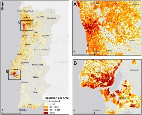
Figure 6. Portugal mainland population distribution – 250 m resolution.

Map of Portugal mainland showing population distribution from 250 m resolution grid and zoomed results for Lisbon and Oporto metropolitan areas.

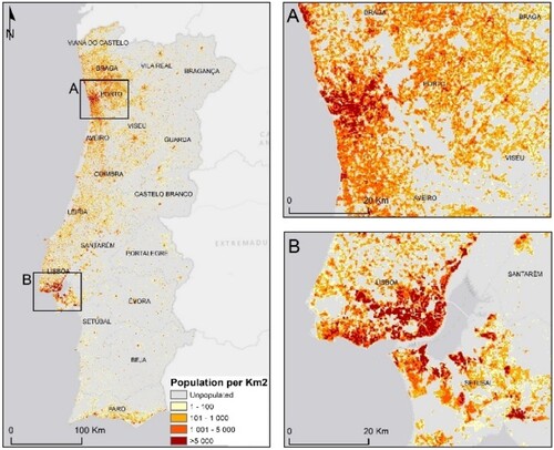
Both population density maps are suggestive of the Portuguese spatial imbalances determined by the unequal distribution of inhabitants. This pattern highlights the spatial concentration in the metropolitan areas of Lisbon and Porto, with cell population densities greater than 1000 inhabitants per sq. km. The population distribution in the present study revealed a high number of small urban areas and low population density and high spatial detail particularly in urban areas. In urban areas, it is possible to identify inhabited areas at the neighborhood/building scale, distinguishing areas of high density (e.g. Parque das Nações) from those of lower population density. In urban areas, uninhabited spaces such as urban parks (e.g. Monsanto or Parque da Cidade do Porto), airports (e.g. Humberto Delgado, Pedras Rubras, Gago Coutinho) or other similar infrastructures are distinguished from inhabited areas. In rural areas, the inhabited areas are limited to the built-up area, with agricultural (e.g. Lezíria do Tejo or Alentejo) and forest (e.g. (Baixo Vouga or Beira Interior Sul) areas remaining without population).

3.3. Accuracy assessment

To validate the estimated resident population, a vector grid made available by the Portuguese Institute of Statistics (INE) with the 2011 Census population was used. This grid was obtained from the population data (georeferenced by building in the 2011 Census Statistics) aggregation into the 250 m and a 500 m grid.

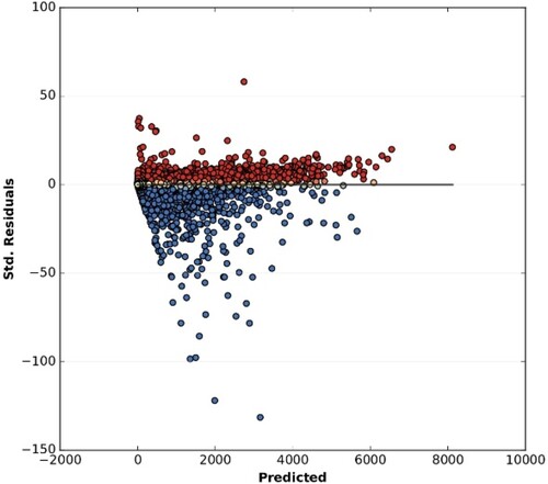
The relationship between estimated and census population counts for the grid cells revealed a high correlation between estimated and census values for both 500 m (R² = 0.994) and 250 m (R² = 0.986) grids. In general terms, over and underestimations reveal reduced absolute deviations (Figure 7 and Figure 8). In both resolutions, an underestimation of the original census data was observed, with a reduced number of positive and negative outliers.

Figure 7. Graph of residuals (model over and under predictions) in relation to predicted dependent variable for 250 m resolution model.

Graphic showing positive residuals in red and negative residuals in blue in relation to predicted dependent variable for 250 m resolution model.

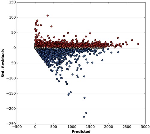
Figure 8. Graph of residuals (model over and under predictions) in relation to predicted dependent variable for 500 m resolution model.

Graphic showing positive residuals in red and negative residuals in blue in relation to predicted dependent variable for 500 m resolution model.

The absolute error follows a normal distribution for the 250 and 500 m resolution population grids, and there are only 17% and 29% of non-zero values.

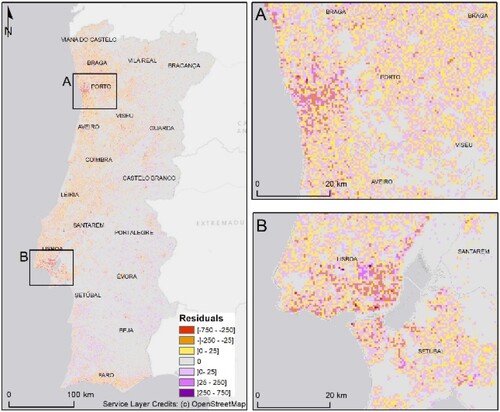
In Figure 9 and Figure 10, it is possible to verify that the distribution of the highest residuals is associated with urban areas.

Figure 9. Residuals map (model over and under predictions) – 250 m resolution.

Map of Portugal mainland showing residuals from 250 m resolution grid and zoomed results for Lisbon and Oporto metropolitan areas.

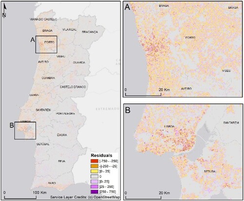
Figure 10. Residuals map (model over and under predictions) – 500 m resolution.

Map of Portugal mainland showing residuals from 500 m resolution grid and zoomed results for Lisbon and Oporto metropolitan areas.

Accuracy results (Table 3) indicate that the 500 m resolution population grid has the lowest precision, with the highest MAE and RMSE (8.96 and 14.86). The 250 m resolution population grid has the best overall performance. It has the highest precision, with the lowest MAE (6.02) and RMSE (5.98). On both grids, the negative bias denotes the tendency towards an underestimation (MALPE −2.99 and −4.34).

Table 3. Error measurements.

Resolution	MAE	RMSE	MALPE
500 m	8.96	14.26	−2.99
250 m	6.02	5.98	−4.34

4. Discussion

The results obtained are in line with similar studies carried out by INE for Portugal with a kilometre grid (GEOSTAT, 2011).

However, the advantage of this approach consists in the possibility of creating population grids with different resolutions from open data with a relatively simple and user-friendly computational model that can be applied by any user with beginner’s skills in geographic information systems. The model proposed assumed that for each enumeration unit the number of persons per housing unit is relatively homogeneous. Comparison of the estimated population, for the 250 and 500 m resolution grids with population numbers observed in the 2011 Census, shows over and underestimations of population, which can be related to limitations of the approach used.

First, the population totals for Portugal mainland are always different in the 250 and 500 m model and census grids. The difference between census 250 and 500 m resolution grids can be explained by the set of cells (14,128 pixels in the 250 m grid and 42,118 pixels in the 500 m grid) where the population was not calculated for statistical confidentiality reasons. The total estimated population, for the 250 and 500 m grids revealed an underestimation when compared with 2011 census grids.

The districts of Bragança, Castelo Branco, Coimbra, Évora and Vila Real show an underestimation of the population with a resolution of 500 m and a slight overestimation with a resolution of 250 m. The districts of Aveiro, Braga, Guarda, Leiria, Lisbon, Portalegre, Porto, Santarém, Setúbal, Viana do Castelo and Viseu display an underestimation of the population, decreasing significantly between the 500 and 250 m resolution models. This decrease may indicate that in the districts with the highest population density, better results are obtained with higher resolutions. The greatest population overestimations are found in the districts of Beja and Faro. The district of Faro stands out with a high overestimation of the population (5.7%) which can be explained by the specialization of the economy of the Algarve region in tourism and in tourist settlement. The touristic resorts and villages represent in the model a high set of addresses that justify the overestimation of the population.

One of the problems with the approach adopted was found in the mismatch between the number of dwellings in the statistical subsections and the number of registered addresses. This mismatch resulted in an overestimation of the population and may be due to a temporal mismatch between the census and the construction of a set of new buildings.

5. Conclusions

The spatial aggregation of addresses open data to produce population distribution maps with a fine spatial resolution resulted in reliable grids, created in a simple and fast way, which is a major contribution towards cost-saving, time-saving, and scientific sound. The proposed methodology makes it possible to produce up-to-date and reliable population estimates, between censuses, if there are new data on addresses and the auxiliary variable relative to the weight of the population/population density is coherent in time and space. In contexts of urban expansion and/or urban regeneration with significant changes in urban planning parameters, the methodology can be applied if the weights of population density can be obtained from other proxy variables, namely the indexes of master plans.

Although the results prove to be promising, there are challenges and future improvements to consider regarding data and spatial granularity. Further work needs to carry out to increase the resolution of the grids to 100, 50 m or less and on the use of auxiliary information regarding the addresses and the number of housing units based on LíDAR surveys through mobile mapping or collection of georeferenced (360°) panoramic images.

In this context, the dissemination of addresses open data will allow to obtain gridded population distribution maps that will enhance and boost the use of grids than were obtained using other models.

Finally, the use in this study of the resident population variable can be easily reused for other variables such as the number of buildings, number of accommodations, number of floors or population by age group.

Software

The development of the QGIS plugin was done in Python 2.7, using the PyQt4 API. The maps were generated in QGIS v3.14 via the Print Composer tool.

Acknowledgements

The authors would like to thank Statistics Portugal (Instituto Nacional de Estatística – INE), for providing the data.

Disclosure statement

No potential conflict of interest was reported by the author(s).

Data availability statement

The data that support the findings of this study are openly available in Statistics Portugal Atom Service at http://inspire.ine.pt/AD/atom/downloadservice.xml. All census data (alphanumeric and geographic data from BGRI) were downloaded from the platform supported and maintained by I.N.E. (Statistics Portugal available at http://mapas.ine.pt/download/index2011.phtml). The data used are freely available for download from this source.

Additional information

Funding

This work was supported by Fundação para a Ciência e a Tecnologia (grant references: UIDB/00295/2020 and UIDP/00295/2020).

Notes

1 http://inspire.ine.pt/AD/atom/downloadservice.xml.

2 http://mapas.ine.pt/download/index2011.phtml.

References

- Bakillah, M., Liang, S., Mobasheri, A., Jokar Arsanjani, J., & Zipf, A. (2014). Fine-resolution population mapping using OpenStreetMap points-of-interest. International Journal of Geographical Information Science. https://doi.org/10.1080/13658816.2014.909045
- Biljecki, F., Arroyo Ohori, K., Ledoux, H., Peters, R., & Stoter, J. (2016). Population estimation using a 3D city model: A multi-scale country-wide study in the Netherlands. PLoS One, 11(6), e0156808. https://doi.org/10.1371/journal.pone.0156808
- Calka, B., Costa, J., & Bielecka, E. (2017). Fine scale population density data and its application in risk assessment. Geomatics, Natural Hazards and Risk, 8(2), 1440–1455. https://doi.org/10.1080/19475705.2017.1345792
- Deng, C., Wu, C., & Wang, L. 2010. Improving the housing–unit method for small–area population estimation using remotesensing and GIS information. International Journal of Remote Sensing, 31, 5673–5688.
- Gallego, F. (2010). A population density grid of the European Union. Population and Environment, 31(6), 460–473. https://doi.org/10.1007/s11111-010-0108-y
- Gaspar, J. (1987). Portugal: os próximos 20 anos. Ocupação e organização do espaço – Retrospectiva e Tendências (Vol. 1). Fundação Calouste Gulbenkian.
- GEOSTAT 1A. (2011). ESSnet project GEOSTAT – Representing census data in a European population grid (1. Final report for A 2010–2011). European Statistical System.
- Lloyd, C., Catney, G., Williamson, P., & Bearman, N. (2017). Exploring the utility of grids for analysing long term population change. Computers, Environment and Urban Systems, 66, 1–12. https://doi.org/10.1016/j.compenvurbsys.2017.07.003
- Lloyd, C., Sorichetta, A., & Tatem, A. (2017). High resolution global gridded data for use in population studies. Scientific Data, 4(1), 170001. https://doi.org/10.1038/sdata.2017.1
- Martin, D., Lloyd, C., & Shuttleworth, I. (2011). Evaluation of gridded population models using 2001 Northern Ireland census data. Environment and Planning A, 43(8), 1965–1980. https://doi.org/10.1068/a43485
- Norman, P., Rees, P., & Boyle, P. (2003). Achieving data compatibility over space and time: Creating consistent geographical zones. International Journal of Population Geography, 9(5), 365–386. https://doi.org/10.1002/ijpg.294
- Schug, F., Frantz, D., van der Linden, S., & Hostert, P. (2021). Gridded population mapping for Germany based on building density, height and type from Earth observation data using census disaggregation and bottom-up estimates. PLoS One, 16(3), e0249044. https://doi.org/10.1371/journal.pone.0249044
- Smith, S., & Cody, S. (1994). Evaluating the housing unit method: A case study of 1990 population estimates in Florida. Journal of the American Planning Association, 60(2), 209–221. https://doi.org/10.1080/01944369408975574
- Smith, S., Nogle, J., & Cody, S. (2002). A regression approach to estimating the average number of persons per household. Demography, 39(4), 697–712. https://doi.org/10.1353/dem.2002.0040
- Tu, W., Liu, Z., Du, Y., Yi, J., Liang, F., Wang, N., Qian, J., Huang, S., & Wang, H. (2022). An ensemble method to generate high-resolution gridded population data for China from digital footprint and ancillary geospatial data. International Journal of Applied Earth Observation and Geoinformation, 107, 102709. ISSN 1569-8432. https://doi.org/10.1016/j.jag.2022.102709
- Wardrop, N., Jochem, W., Bird, T., Chamberlain, H., Clarke, D., Kerr, D., Bengtsson, L., Juran, S., Seaman, V., & Tatem, A. (2018). Spatially disaggregated population estimates in the absence of national population and housing census data. Proceedings of the National Academy of Sciences, 115, 3529–3537. https://doi.org/10.1073/pnas.1715305115